Comparison of forest canopy height profiles in a mountainous region of Taiwan derived from airborne lidar and unmanned aerial vehicle imagery

Abstract

Tree height is essential for assessing carbon budgets and biodiversity. One of the most commonly used assessment methods is a field survey. However, this approach is extremely challenging for obtaining highly accurate estimates in forests with tall and dense canopies. In this study, we utilized airborne remotely sensed mean canopy height (MCH) spatial coverage acquired by high-cost airborne light detection and ranging (lidar) and low-cost unmanned aerial vehicle (UAV) sensors to quantify the tree height for a 590-ha complex tropical forest in the mountainous region of central Taiwan. The performances of the acquisition techniques were evaluated by comparing the statistical relationships of MCH from lidar and MCH from UAV with the concurrently obtained field mean tree height measurement (MTH) at the plot (25 × 20 m) scale. In addition, we further analyzed the forest structural variables that may influence lidar and UAV MCHs by using a general linear model. The results showed that both MCHs derived from lidar and UAV accurately estimated MTH. MCH from UAV had a superior performance to that of a small model offset, and the slope of the model fit line was close to one, which was possibly due to the finer spatial resolution of the UAV imagery. MCH from lidar may be utilized to delineate the entire vertical profile of a forest stand, but MCH from UAV can only detect the upper half of the canopies. This is a result of instrument and data differences. General linear model statistics revealed that the maximum stand height and mean tree age may be the major forest stand structure determinants affecting MCH estimates, which might indicate that the airborne estimations of mean canopy height are mainly governed by large trees within a forest stand.

Keywords:

• Canopy height
• forest structure
• general linear model
• relative variable importance (RVI)
• tree height

1. Introduction

Tree height has long been recognized as a key variable in forest ecology and management, and is associated with species diversity (King, Wright, and Connell 2006; Wolf et al. 2012), forest biomass (Gwenzi et al. 2017; Messinger, Asner, and Silman 2016), carbon stocks (Chave et al. 2005; Marc et al. 2019) and timber resources (Nilsson 1996). It is commonly assessed from the ground using a telescopic height pole, a clinometer or a laser altimeter (Clark and Clark 2001; Andersen, Reutebuch, and McGaughey 2006; Larjavaara and Muller-Landau 2013). Unavoidably, these conventional field methods are technically challenging in settings with tall and dense canopies (Larjavaara and Muller-Landau 2013). In addition, this type of approach is time-consuming and labor intensive, which makes long-term or large spatial scale monitoring difficult.

Airborne light detection and ranging (lidar) is an active remote sensing survey technique that is commonly applied to model the three-dimensional (3D) perspective of an object of interest. Lidar can precisely measure multiple vertical layers of a forest canopy structure from the top (digital surface model (DSM)) to the bottom (digital terrain model (DTM)) (Leitold et al. 2015). The difference between these two layers is commonly known as the canopy height model (CHM) (Lefsky et al. 2002). The DTM is relatively stable over a long period of time, but it may change rapidly due to disturbances and seasonality. In recent years, lidar has been heavily utilized for forest height mapping at the regional scale (Wulder et al. 2012). However, the main downsides of lidar are its relatively low flexibility in data acquisition due to flight-related logistics (e.g., aviation regulations) and its high cost, which may make the approach impractical for periodic and long-term forest inventories in some regions.

Applications of unmanned aerial vehicle (UAV) systems for forest surveys were officially documented in the early 2000s (Whitehead and Hugenholtz 2014). The strengths of UAV data acquisition include its high spatial resolution, flexibility in flight scheduling and low cost, making it an ideal system for frequent forest monitoring at an intermediate spatial extent (e.g., 100–100,000 ha) (Messinger, Asner, and Silman 2016; Torres-Sánchez et al. 2015; Hardin et al. 2019). In addition, a UAV can fly steadily at a very low altitude (< 50 m) below the cloud coverage. These advantages of UAV operations may compensate for the challenges faced while using lidar. Therefore, UAV is feasible for terrestrial mapping tasks (see a comprehensive synthesis by Singh and Frazier (2018)) including a wide range of vegetated settings such as farmland (Huang et al. 2018), grassland (Lu and He 2018), and humid tropical regions (Shahbazi, Théau, and Ménard 2014; Zahawi et al. 2015). Combining photogrammetry and computer vision techniques (e.g., Structure from Motion, SfM) (Westoby et al. 2012), a sophisticated 3D perspective of forest structure can be constructed from dense cloud points derived from ultrahigh spatial resolution (5–20 cm) UAV imagery (Lisein et al. 2013). The performance of SfM integration with geostatistics used to portray the DSM of a small forest stand in past works was comparable to lidar, and the UAV was deemed an adequate low-cost alternative for forest stand surveys (Singh et al. 2016; Wallace et al. 2016; Singh et al., 2018).

Comparisons of the feasibilities of lidar and UAV for forest height mapping have been conducted in previous studies (Zarco-Tejada et al. 2014; Wallace et al. 2016; Bridal et al., 2017). However, those works mostly focused on one type of vegetation (e.g., broadleaf or conifer forests) and the underlying topography was quite homogeneous. Thorough investigations on different vegetation types and complex terrains are very limited. Therefore, in this study, we performed a comprehensive analysis to assess the feasibility of using UAV imagery to assess the mean forest stand structure profile (mean canopy height, MCH) by comparing it to lidar in a heterogeneous mountainous setting with mosaics of secondary broadleaf forests and broadleaf and conifer plantations. In addition, we also studied the stand characteristics that may affect the remotely sensed estimates of MCH using lidar and UAV. The novel approaches conducted in this study may facilitate a thorough understanding of the strengths, weaknesses and extents of these two most commonly used airborne forest mapping systems.

2. Methods

2.1 Study site

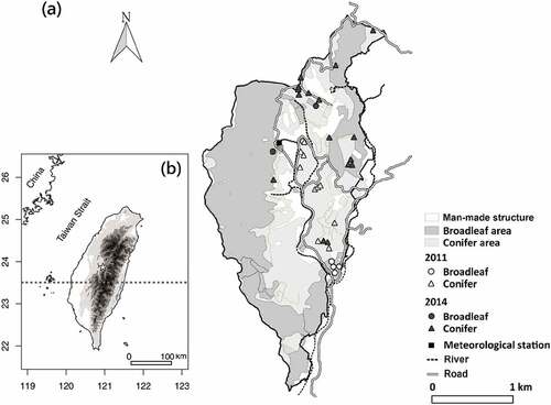
The 590 ha study site, known as the Lienhuachih Experimental Station, is located in central Taiwan (23°54.9ʹ N, 120°52.8ʹ E) (Figure 1) within a mean elevation (± standard deviation, sd) of 660.8 ± 105.1 m above sea level (a.s.l.) ranging from 300 to 1100 m a.s.l., and a mean (± sd) slope of 29.2 ± 14.1° (range = 0–84.9°). The vegetation types are representative of the lower mountainous region of Taiwan (Chang, Wang, and Huang, 2013) and consist of secondary broadleaf forests (52.3%), and broadleaf (5.5%) and conifer (42.2%) plantation stands (Taiwan Forestry Research Institute: https://www.tfri.gov.tw). The mean annual precipitation and air temperature (± sd) of the site are 2313 (± 679) mm y⁻¹ and 20.7 (± 0.8) °C, respectively, according to long-term on-site meteorological records (1961–2016). Primary rainfall (more than 85% of the mean annual precipitation) was received in the spring and summer (March-September) (Figure S1). The terrain is quite steep (32–36°), and the main substrate type is Typic Paleudults. The dominant broadleaf tree species in the secondary forests are Pasania nantoensis, Engelhardtia roxburghiana, Schefflera arboricola, Schima superba and Cyclobalanopsis pachyloma (Chang et al. 2010); the broadleaf and conifer species of the plantations established in 1936–1999 are Cunninghamia lanceolata, Calocedrus formosana and Michelia formosana. Most of the tree species in the experimental station are evergreen, and no apparent seasonal defoliation was observed (McEwan et al. 2011).

Figure 1. (a) The study site, Lienhuachih Experimental Station, located in (b) the mountainous region of central Taiwan (the dashed gray line is the Tropic of Cancer). The sample sites are shown as circles (broadleaf species plots) and triangles (conifer species plots).

2.2 Field measurements

The height of each tree, with a diameter at breast height (DBH, defined as 130 cm above the ground level) ≥ 5 cm within 15 and 18 0.05 ha (25 × 20 m) inventory plots at the experimental station, was assessed in 2011 and 2014, respectively (Figure 1), and no plot was sampled in both years. The center of each plot was geo-referenced using a high precision (10 cm accuracy in the real-time kinematic (RTK) mode) global positioning system (GPS, GeoXH, Trimble Inc., CA, USA). Trees were measured using a 15 m expandable measuring pole (model A-15, Senshin Industry, Osaka, Japan) from the forest floor to the highest live leaf or twig (Clark and Clark 2001). If the height was greater than the pole, a second pole was connected using a pipe. Trees taller than 30 m were not found in our field inventory. The ages of stands were derived from local government records (Taiwan Forestry Research Institute: https://www.tfri.gov.tw).

2.3 Airborne imagery

The airborne lidar data were acquired on 16 August 2011 via a national scale geological inventory project administered by the Taiwan Central Geological Survey (see Table 1 for the specifications of the sensor). The original point cloud data were preprocessed and resampled to a 1-m spatial resolution by the data provider. According to the data user manual (Hou et al. 2014), 40% or greater overlap was required for each neighboring flight stripe. The lidar first return and ground points were interpolated using adaptive kriging (SCOP++, Department of Geodesy and Geoinformation, Vienna, Austria) to generate the DSM and DTM, respectively; the CHM from lidar was derived by calculating the difference between them. The accuracy of DSM was ≤ 22.5 cm as compared with measurements from a high precision GPS; the quality was visually assessed to verify potential erroneous point cloud data, such as extremely high or low values compared to values of the nearby features before data product distribution (Hou et al. 2014).

Table 1. The instrument specifications of lidar (light detection and ranging) and the UAV (unmanned aerial vehicle) and the characteristics of the acquired data. The short dashes indicate information that is not applicable.

Characteristics	Lidar	UAV
Ground control point	9
Acquisition date	2011/08/16	2014/12/23
Altitude (a.s.l.)	2430 m	1110 m
Frequency	25.8–38.2 kHz
Number of images	-	1217
Side overlap	70%	80%
Flight speed	51 m s^−1	25 m s^−1
Instrument	Leica ALS60	Canon PowerShot S110
Ground sampling distance	1 m (1–2 pts m^−2)	0.13 m
Focal length	-	5 mm
FOV	40.0	17.8

The UAV mission was carried out on 23 December 2014 (Table 1). For the spatial continuity of the data, 80% forward and side overlaps were programmed before the flight, and data were georeferenced using a high precision GPS (GeoXH, Trimble Inc., CA, USA) to measure nine ground control points (GCPs). The UAV point clouds were interpolated and resampled to generate 13-cm orthophotography and the DSM in Pix4D (Figure 2, Pix4D SA, Lausanne, Switzerland). The mean x, y and z errors were ≤ 3 cm by referring to the GCPs. We aggregated the 13 cm spatial resolution DSM derived from UAV to 1 m using the nearest neighborhood technique, and the CHM of UAV was then derived by subtracting the DSM from UAV (top of the canopies) from the lidar DTM (ground surface). To match the ground surveyed data, pixels of the CHMs from UAV and lidar were both aggregated with a low pass filter to the field plot size (25 m × 20 m) to generate the mean canopy height (MCH) using Geographical Information Systems (GIS) software (QGIS v. 2.18.1, http://www.qgis.org) for further analyses.

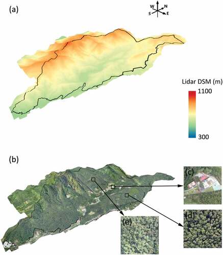
Figure 2. (a) The DSM of the study site derived from lidar point cloud data. (b) The three-dimensional point cloud data of the study site acquired from a digital camera mounted on an unmanned aerial vehicle. The subsets show (c) the research center building of the site, (d) a Calocedrus formosana plantation and (e) a secondary broadleaf forest.

2.4 Remotely sensed delineation of the height structure of forest stands

The qualities of UAV- and lidar-measured MCHs were first evaluated by comparing the relationships to spatiotemporally corresponding average field measured mean tree heights (MTH). The normality of the datasets was tested by the Shapiro-Wilk’s test, which was designed to examine small sample sizes (Oztuna, Elhan, and Tuccar 2006; Yap and Sim 2011). The statistical analysis was conducted using a general linear model (R package stats v. 3.3.3, Stanford University; http://www.r-project.org/) and a flexible generalization of an ordinary linear regression to investigate the MTH acquired from 2011 and 2014 and the spatially corresponding MCH from lidar and UAV. In addition, Moran’s I (Haining 1990) was applied to determine the effect of spatial autocorrelation on the generalized linear model if it violated the basic assumption for a standard statistical test that data should be independent and identically distributed (iid), or an alternative approach such as generalized additive models or a classification tree analysis may be applied (Segurado, Araújo, and Kunin 2006). We also assessed the impacts of local topographic characteristics (derived from 1-m lidar DTM), including the plot scale mean slope (degree) and a Terrain Ruggedness Index (TRI) (Riley, Degloria, and Elliot 1999), and the sd of elevation. The terrain ruggedness metric was calculated by referring to the following eq. 1:

(1) $\text{TRI}={\displaystyle \sum {\left[\left(x_{ij}-x_{00}\right)\right]}^{1/2}}$(1)

where x_ij are the elevations of neighbor cells to the elevation of the center cell x₀₀. Moreover, we further compared the forest stand height structure within a plot (the shortest tree (Q₀), 25th percentile (Q₂₅), mean, median (Q₅₀), 75th percentile (Q₇₅) and the tallest tree (Q₁₀₀)) with the spatially corresponding canopy height pixels derived from lidar or the UAV.

2.5 Stand structure variables and MCH estimation

To assess forest structure variables that may influence canopy height estimates from airborne remote sensing, we applied the generalized linear model again to investigate the relationship between the stand structure variables (plot averaged tree age and height (MTH), stand density, the sd of MTH (MTH_sd), Q₀, Q₂₅, mean, Q₅₀, Q₇₅ and Q₁₀₀) and the MCH of lidar and UAV. To remedy the potential effect of collinearity (the correlation between two independent forest structure variables), variance inflation factors (VIFs) were used to investigate the relationships among variables (i.e., VIF > 5 indicating a high correlation, Akinwande, Dikko, and Samson 2015) (eq. 2). VIFs were calculated by an independent variable (MTH), and they were built against every other independent variable (e.g., the mean tree age, stand density, MTH_sd, Q₀, Q₂₅, mean, Q₅₀, Q₇₅ and Q₁₀₀) in the regression model. We then calculated the VIF factor for x independent variables with the following formula (eq. 2):

(2) $\mathrm{V}\mathrm{I}\mathrm{F}=\frac{1}{1-R{\hspace{0.17em}}_x^2}$(2)

where “x” is the predictor (e.g., plot averaged tree age, stand density and MTH, MTH_sd, Q₀, Q₂₅, mean, Q₅₀, Q₇₅ and/or Q₁₀₀), and R² is the coefficient of determination. Additionally, Moran’s I was also applied to corroborate the spatial autocorrelation of the variables. We arbitrarily selected variables yielding VIFs < 5 with insignificant spatial autocorrelations and injected them into the generalized linear model. The model assumed MCH to be a Gaussian distribution and was developed with a set of selected variables (eq. 3) as follows:

(3) $\mathrm{M}\mathrm{C}\mathrm{H}\cdot =\cdot \mathrm{a}+{\beta }_1\mathrm{v}\mathrm{a}{\mathrm{r}}_1+{\beta }_2{var}_2\cdot +...$(3)

where MCH is the mean canopy height derived from lidar or UAV imagery, α is the constant coefficient and β_i are coefficients of the VIF-screened explanatory variables. The Akaike’s Information Criterion (AIC) (Akaike 1974) was used to assess the contribution of each forest structure variable to MCH. We also standardized these variables and used ΔAIC (increment in AIC relative to the lowest AIC model) for variable selection and model development (ΔAIC < 2, R MuMIn package, Burnham and Anderson 2002). All these statistical analyses were conducted in the R stats package. To evaluate the contribution of each salient variable to the MCH estimation, we used the relative variable importance (RVI) to identify important variables. The RVI was based on the variables’ frequency of occurrence and was calculated from the ranks of all variables within a confidence set of models (Yates et al. 2015; Gehman et al. 2017).

3. Results

3.1 Field inventory

Within the 3 year time gap of 2011 (concurrently with lidar observations) and 2014 (UAV observations), 1173 and 1180 trees were measured, respectively (see Table 2 for detailed statistics). This temporal gap was negligible since the difference between the plot-average tree ages was insignificant (analysis of variance (ANOVA), p > 0.05). A similar statistical pattern was observed from stand densities but not the mean DBHs (p = 0.036) and tree heights (p = 0.001). The normality test indicated a normal distribution for field datasets acquired in both years (for 2011: Shapiro-Wilk normality test: W = 0.96, p = 0.74, skewness = 0.17, kurtosis = −0.94; for 2014: W = 0.97, p = 0.94, skewness = −0.18, kurtosis = −0.31).

Table 2. Summary of characteristics of trees in the sampled plots. The numbers in parentheses are standard deviations. Superscripted asterisks indicate significantly different (p ≤ 0.05) estimates compared to the field observations.

	Field		Lidar	UAV
Year	2011	2014	2011	2014
Sample size (plot or pixel)	15	18	7500	72,410
Stand density (# ha^−1)	1516 (556)	1455 (635)
Age (year)	34.3 (4.8)	41.1 (14.4)
DBH (cm)	12.5 (3.8)	16.2 (6.7)
Tree height (m)
Q0	3.5 (1.9)	4.8 (3.3)	2.6 (2.5)	12.5 (4.5)*
Q25	8.5 (3.0)	10.1 (3.8)	11.1 (4.0)	16.5 (4.1)*
Mean	9.4 (2.7)	12.1 (3.6)	11.4 (4.0)	17.5 (4.0)*
Q50	10.2 (3.1)	16.2 (3.5)	12.8 (4.3)	17.8 (4.0)
Q75	11.5 (3.4)	18.2 (3.7)	14.5 (4.4)	19.1 (3.7)
Q100	15.5 (2.7)	22.3 (4.5)	18.4 (4.4)	23.0 (3.4)

3.2 Remotely sensed delineation of the height structure of forest stands

Spatial autocorrelations were insignificant for MCH from lidar (Moran’s I = 0.12, p = 0.07) and MCH from UAV (Moran’s I = −0.22, p = 0.93), which permitted the use of the generalized linear model to assess the feasibility of utilizing the airborne remotely sensed canopy height (MCHs from lidar and UAV) to estimate the field-measured tree height at the plot scale. The MCHs from lidar and UAV both adequately estimated the field MTH (p < 0.001) (Figure 3) with comparable explanatory powers (R² = 0.77 and 0.74, respectively) (Figure 4). Additionally, the MCH from UAV was more similar to the ground measurements since the slope was closer to one (0.77 vs. 0.65), with a smaller offset (0.18 vs. 2.01). The RMSE values for lidar and UAV were 1.78 m and 1.77 m, respectively; the RMSE values for lidar/UAV for broadleaf and conifer forest stands were 1.88/1.44 m and 1.86/1.56 m, respectively. The topographic complexity analysis indicated that there were no significant relationships between the lidar and UAV model residuals (Figure 4) and the plot scale mean slope (R² ≤ 0.24, p ≥ 0.07) and the TRI (R² ≤ 0.18, p ≥ 0.11), and the standard deviation of elevation within each plot (R² ≤ 0.17, p ≥ 0.13) (Figure S2); however, the relationships were more pronounced for the lidar model (mean R² = 0.2 vs. R² = 0.03 for the UAV model).

Figure 3. (a) A sample transect (120°53ʹ26.16,” 23°55ʹ9.84” to 120°53ʹ29.40,” 23°55ʹ9.84”) of UAV canopy imagery (the green-colored inset in (b)), its spatially corresponding lidar DTM, and lidar and UAV point cloud data. (b) Derived lidar and UAV canopy height models through the transect.

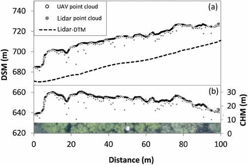
Figure 4. The comparisons between temporally corresponding field-measured mean tree heights (MTH) and the remotely sensed mean canopy height model (MCH) derived from (a) lidar (acquired in 2011) and a (b) UAV (2014). Solid and dashed lines are the regression and 1:1 lines, respectively; horizontal and vertical error bars indicate standard deviations that were calculated from all pixels in each plot (20 m × 25 m).

To understand the deviation between the UAV/lidar and field inventory data, we derived the differences between them and used a t-test to investigate whether the means (Q₀, Q₂₅, mean, Q₅₀, Q₇₅ and Q₁₀₀) differ from 0. Our analysis of forest stand height structure delineation indicated that lidar but not UAV imagery could be utilized to fully portray the canopy height profile in the study site (Table 2). There were no significant differences (p > 0.05) throughout the entire forest stand vertical profile (Q₀, Q₂₅, mean, Q₅₀, Q₇₅ and Q₁₀₀) between the field tree height and lidar canopy estimates, with a mean (± sd) absolute difference of 1.6 ± 0.8 m. However, the canopy height could only be delineated for the upper layers (Q₅₀, Q₇₅ and Q₁₀₀) of field-measured tree heights (p > 0.05), with a mean (± sd) absolute difference of 1.5 ± 1.0 m.

3.3 Stand height structure variables and MCH estimation

In this study, we investigated the contributions of forest stand structures to MCHs from lidar and UAV estimates using the generalized linear model. Variance inflation factors (VIFs) of a set of variables, including the tree age, stand density, MTH, MTH_sd, Q₀, Q₂₅, mean, Q₅₀, Q₇₅ and Q₁₀₀, were derived to assess the collinearity with the exclusion threshold of VIF > 5. The results showed that the tree age, stand density, MTH_sd, Q₀ and Q₁₀₀ are salient variables for the generalized linear model (Figure 5) without a pronounced (p ≤ 0.05) spatial autocorrelation according to Moran’s I statistics. However, besides the tree age, none of these stand structural variables were correlated with the MCHs from lidar and UAV, and the statistical relationships among these variables may not be consistent between the lidar and UAV plots (Figures 1 and S3). There were two lidar and four UAV generalized linear models with ΔAIC < 2. The intercepts of these models were all set to 0; the pseudo R² is a relative measure among similar models indicating how effectively the model explains the data variation (Table 3). Overall, Q₁₀₀ (RVI_lidar = 0.97 and RVI_UAV = 0.97) and age (RVI_lidar = 0.68 and RVI_UAV = 0.52) yielded high RVIs and were included in all selected generalized linear models. MTH_sd and Q₀ were also pivotal for delineating MCHs from lidar and UAV variations and were added into some of the lidar and UAV generalized linear models, and the stand density was only important for one UAV generalized linear model. Although the full models with all the VIF-screened forest stand structure variables were superior to other models in terms of model fitness (pseudo R²), the ΔAICs of both models were greater than 2 (Table 3).

Table 3. The generalized linear models with a subset of selected field forest stand structural attributes (Figure 6 yielding ΔAIC < 2) and the full models (lidar_Full and UAV_Full) using all the variables for estimation of MCHs from lidar and UAV. Weight is the Akaike weight; the p-values of Moran’s I are all greater than 0.05. AIC and MTH_sd are the abbreviations for the Akaike’s Information Criterion and the stand deviation of the plot scale mean tree height, respectively; and Q₀ and Q₁₀₀ are the minimum and maximum heights of trees within a plot, respectively.

Model	Coefficients					AIC	ΔAIC	Weight	Moran’s I	Pseudo R^2
	Age	Stand density	MTHsd	Q0	Q100
Lidar	0.58			0.51	0.77	66.7	0	0.34	0.08	0.83
	0.41		−0.64		1.25	66.8	0.1	0.32	0.11	0.85
LidarFull	0.53	0.22	−0.43	0.17	1.05	67.9	1.2	0.19	0.08	0.86
UAV	0.39				0.62	85.5	0	0.2	−0.03	0.80
	0.41	−0.24			0.43	86.1	0.6	0.15	−0.05	0.83
	0.37			−0.14	0.72	87.0	1.5	0.1	−0.01	0.81
	0.31		0.12		0.67	87.1	1.6	0.09	−0.02	0.81
UAVFull	0.42	−0.25	−0.05	−0.18	0.53	89.4	3.9	0.03	−0.01	0.84

Figure 5. The relative variable importance (RVI) of selected forest stand variables for the development of the generalized linear model for MCHs from lidar and UAV.

4. Discussion

4.1 Estimation of tree height using airborne imagery

Previous studies have demonstrated that the performances of lidar and UAV in estimating tree heights were comparable, and they were verified at the individual and stand scales, yielding model fitness values (R²) ranging from 0.68 to 0.94 (Lisein et al. 2013; Zarco-Tejada et al. 2014; Ota et al. 2015; Wallace et al. 2016; Birdal, Avdan, and Türk 2017). In this study, we performed comprehensive analyses and further investigated the feasibilities of delineation of mean tree height profiles of different vegetation structures (secondary broadleaf forest stands and broadleaf and conifer forest plantations) in mountainous terrain; this was done with airborne lidar and UAV imagery using statistical models and photogrammetry technology, respectively, with the availability of a fine spatial resolution lidar-derived DTM. Both models of MCH from lidar and UAV produced similar model fitness values, and the MCH from UAV was more congruent with the field-measured MTH. The model yielded a smaller offset, and the slope was close to one. Although the differences of MTHs (2.7 m) of 2011 and 2014 were statistically significant (Table 2), it should not be a crucial issue for validation. The high spatial resolution (13 cm) of UAV imagery may play a significant role in the delineation of the forest canopy height profile, which may better delineate the highest point of a canopy. However, the relatively coarse resolution (1 m) of lidar data might generate locational errors that lack a close fit to the maximum heights of canopies. We note that the MCHs from lidar and UAV were smaller than the field-measured MTH (Figure 4). This might be due to the averaging procedure from CHM to MCH, where many low CHM values (e.g., the understory shrub layer or even the forest floor) were included in the calculation. Terrain complexity (within the plot mean slope and the Terrain Ruggedness Index, and within the plot sd of elevation) had no (UAV) or marginal (lidar) influences on the MTH estimations (Figure S2). However, the accuracy of the DTM in this mountainous region with dense canopies may induce uncertainty into tree height estimations (Kraus and Pfeifer 1998; Su and Bork 2006; Spaete et al. 2011).

4.2 Canopy height observations using lidar and a UAV

There are trade-offs in quantifying forest stand structures using lidar and a UAV. Lidar is known for detailed quantifications of forest canopy vertical profiles (Lefsky et al. 2002; Carrasco et al. 2019), which are pivotal for biodiversity conservation, forest ecosystem management and estimations of the carbon budget (Hyde et al. 2006; Hakkenberg et al. 2016; Torresan et al. 2016). Laser beams from the sensor can penetrate dense canopies, which allow for the delineation of a stratified forest with multiple vertical canopy layers (Kellner and Asner 2014). However, the form of a nearly continuous top tree canopy layer in this type of setting prevents in-depth observations of the vertical profile using an optical passive sensor such as the one carried by the UAV in our study (Table 2).

In this study, the UAV was operated at a relatively low altitude to acquire very fine spatial resolution aerial photographs. This high spatial resolution coverage may be closer to the actual tree height at the plot (stand) scale (Figure 4) and may still be feasible for higher canopy layers from Q₅₀ to Q₁₀₀ (Table 2) when compared to the MCH from lidar estimates. Moreover, UAV’s low operation cost (in our case, 21,000 USD and 3,000 USD for one-day missions of lidar and UAV, respectively) may make it a superior system to lidar for many applications. With the availability of spatiotemporally invariant DTM, a UAV may be practical for rapid tree height inventories at an intermediate spatial extent (e.g., 100–100,000 ha) (Messinger, Asner, and Silman 2016; Torres-Sánchez et al. 2015). In the future, the comparison approach conducted in this study should be further applied to an even more densely vegetated forest (leaf area index = 3.6 at the experimental site, Chen, Lin, and Hwong 2007) to further extend the applications of UAV for regional tree and canopy height estimations.

4.3 Influences of the height structure of forest stands on the MCH

To determine the field-measured stand structure variables that affected the airborne MCH estimation, we derived VIFs from an exhaustive list of field-measured variables (plot averaged tree age, stand density, MTH, MTH_sd, Q₀, Q₂₅, mean, Q₅₀, Q₇₅ and Q₁₀₀) and selected those that were independent and spatially uncorrelated. We then combined the RVI and the generalized linear model to assess the ramifications of forest stand height characteristics for MCH estimates. We find that Q₁₀₀, the tallest tree within a plot, is key in governing the tree growth of a site, and it was included in all MCHs from the selected and generalized lidar and UAV linear models (Table 3). The significant role of the largest tree for carbon sequestration of an entire ecosystem has been theoretically and empirically proven using the metabolic scaling theory (Enquist, West, and Brown 2009). In addition, plot-averaged tree ages, which can also be referred as the maturity of a forest and likely affected remotely sensed canopy height estimates, was also a pivotal factor for the airborne canopy height estimation (Figure 5). In forestry, tree age has been commonly utilized as an indirect variable to infer height (Raulier, Pothier, and Bernier 2003). The forests of the experimental station are relatively young and are dominated by secondary broadleaf forests and broadleaf and conifer plantations (McEwan et al. 2011). Tree ages are in general positively correlated to the vertical and horizontal extents of trees (Chen and Rose 1978; Yang et al. 2015).

Our analysis also revealed that the MTH_sd and Q₀ were also important for MCHs from lidar and UAV estimations, and they were included in one of the VIF-screened generalized linear models (Table 3). A high MTH variation may indicate the greater maturity of a forest stand. The MTH variation contributed more to MCH from lidar than from UAV in terms of RVIs (Figure 5), since the sensor may penetrate the top canopy layer and measure the heights of understory trees (Table 2). According to our field observations, the tree with the minimum height (Q₀) was usually a short stature understory tree with a DBH of 5 cm. The high spatial resolution of UAV imagery (13 cm) may be able to detect short stature plants through small canopy gaps (also see Zahawi et al. 2015). Therefore, the spatial resolution played a relatively more significant role (higher RVI) in the MCH from UAV than from lidar (Figure 5). The spatial resolution factor may also explain why the stand density was only crucial for MCH from the UAV but not for the MCH from lidar (Table 3). This is possibly due to the UAV’s superior portrait of forest surface heterogeneity (St-Onge, Audet, and Begin 2015; Zahawi et al. 2015), and it may be able to delineate each tree crown (Wallace et al. 2016) using the UAV (Figure 3(b)).

5. Conclusions

In this study, we investigated the feasibility of utilizing airborne remotely sensed imagery to delineate tree height at the plot scale in a mountainous tropical forest with a mixture of secondary broadleaf forest stands and conifer/broadleaf plantations. We conclude that both MCHs from lidar and UAV are reliable for estimating the field MTH. MCH from UAV is more similar to field observations, and the operation of the UAV has higher flexibility and is less costly. However, lidar is superior to the UAV in terms of forest vertical profile delineation, especially for lower layers. However, lidar’s inevitable limitations include a high cost and difficult logistics, which prevent its widespread practicability. Q₁₀₀ and tree age may be the major forest stand structure determinants used to affect MCH from lidar and from UAV estimates, which might indicate that remotely sensed estimations of the mean canopy height are governed by the large trees within a forest stand. These findings are generic and should be applicable to most cases of airborne forest mapping campaigns, which may assist decision making processes in forest resources management.

Acknowledgements

We thank the editor Dr. Im for handling the manuscript and three anonymous reviewers for providing suggestions that greatly improved the quality of the work. Yu-Huang Wang and Chau-Chin Lin (Taiwan Forestry Research Institute) are acknowledged for providing the UAV imagery. This study was sponsored by grants from the Ministry of Science and Technology of Taiwan (MOST 104-2119-M-002-034-), National Taiwan University (EcoNTU: 10R70604-2, NTU-107L9010) and Research Center for Future Earth, The Featured Areas Research Center Program, Higher Education Sprout Project, Ministry of Education (MOE) in Taiwan.

Disclosure statement

No potential conflict of interest was reported by the authors.

Supplementary material

Supplementary data can be accessed here

Additional information

Funding

This work was supported by the Ministry of Education [The Featured Areas Research Center Program, Higher Education Sprout Project];National Taiwan University [10R70604-2];National Taiwan University [NTU-107L9010];Ministry of Science and Technology (Taiwan) [MOST 104-2119-M-002-034-].

References

- Akaike, H. 1974. “A New Look at the Statistical Model Identification.” IEEE Transactions on Automatic Control 19: 716–723. doi:10.1109/TAC.1974.1100705.
- Akinwande, M. O., H. G. Dikko, and A. Samson. 2015. “Variance Inflation Factor: As a Condition for the Inclusion of Suppressor Variable(S) in Regression Analysis.” Open Journal of Statistics 5: 754–767. doi:10.4236/ojs.2015.57075.
- Andersen, H.-E., S. E. Reutebuch, and R. J. McGaughey. 2006. “A Rigorous Assessment of Tree Height Measurements Obtained Using Airborne Lidar and Conventional Field Methods.” Canadian Journal of Remote Sensing 32 (5): 355–366. doi:10.5589/m06-030.
- Birdal, A. C., U. Avdan, and T. Türk. 2017. “Estimating Tree Heights with Images from an Unmanned Aerial Vehicle.” Geomatics, Natural Hazards and Risk 8 (2): 1144–1156. doi:10.1080/19475705.2017.1300608.
- Burnham, K. P., and D. R. Anderson. 2002. Model Selection and Multimodel Inference: A Practical Information-Theoretic Approach. New York: Springer.
- Carrasco, L., X. Giam, M. Papeş, and K. S. Sheldon. 2019. “Metrics of Lidar-Derived 3D Vegetation Structure Reveal Contrasting Effects of Horizontal and Vertical Forest Heterogeneity on Bird Species Richness.” Remote Sensing 11: 743. doi:10.3390/rs11070743.
- Chang, C.-T., H.-C. Wang, and C.-Y. Huang. 2013. “Impacts of Vegetation Onset Time on The Net Primary Productivity in a Mountainous Island in Pacific Asia.” Environmental Research Letters 8: 045030. doi:10.1088/1748-9326/8/4/045030.
- Chang, L. W., J. H. Hwong, S. T. Chiu, H. H. Wang, K. C. Yang, H. Y. Chang, and C. F. Hsieh. 2010. “Species Composition, Size-Class Structure and Diversity of the Lienhuachih Forest Dynamics Plot in a Subtropical Evergreen Broad-Leaved Forest in Central Taiwan.” Taiwan Journal of Forest Science 25: 81–95.
- Chave, J., C. Andalo, S. Brown, M. A. Cairns, J. Q. Chambers, D. Eamus, H. Fölster, et al. 2005. “Tree Allometry and Improved Estimation of Carbon Stocks and Balance in Tropical Forests.” Oecologia 145: 87–99. doi:10.1007/s00442-005-0100-x.
- Chen, C. M., and D. W. Rose. 1978. “Direct and Indirect Estimation of Height Distributions in Even-Aged Stands.” Minnesota Forestry Research Notes 267: 3.
- Chen, C.-H., T.-C. Lin, and J.-L. Hwong. 2007. “Variations in the Leaf Area Index and Its Effect on Estimations of Primary Production in a Natural Hardwood Forest and a Cunninghamia Lanceolata Plantation at the Lienhuachi Experimental Forest, Central Taiwan.” Taiwan Journal of Forest Science 22(4): 423–439. [in Chinese with English summary].
- Clark, D. A., and D. B. Clark. 2001. “Getting to the Canopy: Tree Height Growth in a Neotropical Rain Forest.” Ecology 82 (5): 1460–1472. doi:10.2307/2680002.
- Enquist, B. J., G. B. West, and J. H. Brown. 2009. “Extensions and Evaluations of a General Quantitative Theory of Forest Structure and Dynamics.” Proceedings of the National Academy of Sciences, USA 106: 7046–7051. doi:10.1073/pnas.0812303106.
- Gehman, A. M., J. H. Grabowski, A. R. Hughes, D. L. Kimbro, M. F. Piehler, and J. E. Byers. 2017. “Predators, Environment and Host Characteristics Influence the Probability of Infection by an Invasive Castrating Parasite.” Oecologia 183 (1): 139–149. doi:10.1007/s00442-016-3744-9.
- Gwenzi, D. E., H. Helmer, X. Zhu, M. A. Lefsky, and H. Marcano-Vega. 2017. “Predictions of Tropical Forest Biomass and Biomass Growth Based on Stand Height or Canopy Area are Improved by Landsat-Scale Phenology across Puerto Rico and the U.S. Virgin Islands.” Remote Sensing 9: 123. doi:10.3390/rs9020123.
- Haining, R. 1990. Spatial Data Analysis in the Social and Environmental Sciences. Cambridge, UK: Cambridge University Press.
- Hakkenberg, C. R., C. Song, R. K. Peet, and P. S. White. 2016. “Forest Structure as a Predictor of Tree Species Diversity in the North Carolina Piedmont.” Journal of Vegetation Science 27 (6): 1151–1163. doi:10.1111/jvs.12451.
- Hardin, P. J., V. Lulla, R. R. Jensen, and J. R. Jensen. 2019. “Small Unmanned Aerial Systems (Suas) for Environmental Remote Sensing: Challenges and Opportunities Revisited.” GIScience & Remote Sensing 56 (2): 309–322. doi:10.1080/15481603.2018.1510088.
- Hou, C.-S., L.-Y. Fei, C.-L. Chiu, H.-J. Chen, Y.-C. Hsieh, J.-C. Hu, and C.-W. Lin. 2014. “Airborne LiDAR DEM and Geohazards Applications.” Journal of Photogrammetry and Remote Sensing 18 (2): 93–108. doi:10.6574/JPRS.2014.18(2).3.
- Huang, C.-Y., H.-L. Wei, J.-Y. Raud, and J.-P. Jhan. 2018. “Use of Principal Components of UAV-acquired Narrow-Band Multispectral Imagery to Map the Diverse Low Stature Vegetation fAPAR.” GIScience & Remote Sensing 56 (4): 605–623. doi:10.1080/15481603.2018.1550873.
- Hyde, P., R. Dubayah, W. Walker, J. B. Blair, M. Hofton, and C. Hunsaker. 2006. “Mapping Forest Structure for Wildlife Habitat Analysis Using Multi-Sensor (Lidar, SAR/ InSAR,ETM+, Quickbird) Synergy.” Remote Sensing of Environment 102: 63–73. doi:10.1016/j.rse.2006.01.021.
- Kellner, J. R., and G. P. Asner. 2014. “Winners and Losers in the Competition for Space in Tropical Forest Canopies.” Ecology Letters 17: 556–562. doi:10.1111/ele.12256.
- King, D. A., S. J. Wright, and J. H. Connell. 2006. “The Contribution of Interspecific Variation in Maximum Tree Height to Tropical and Temperate Diversity.” Journal of Tropical Ecology 22: 11–24. doi:10.1017/S0266467405002774.
- Kraus, K., and N. Pfeifer. 1998. “Determination of Terrain Models in Wooded Areas with Airborne Laser Scanner Data.” ISPRS Journal of Photogrammetry and Remote Sensing 53 (4): 193–203. doi:10.1016/S0924-2716(98)00009-4.
- Larjavaara, M., and H. C. Muller-Landau. 2013. “Measuring Tree Height: A Quantitative Comparison of Two Common Field Methods in A Moist Tropical Forest.” Methods in Ecology and Evolution 4: 793–801. doi:10.1111/2041-210X.12071.
- Lefsky, M. A., W. B. Cohen, G. G. Parker, and D. J. Harding. 2002. “Lidar Remote Sensing for Ecosystem Studies.” BioScience 52: 19–30. doi:10.1641/0006-3568(2002)052[0019:LRSFES]2.0.CO;2.
- Leitold, V., M. Keller, D. C. Morton, B. D. Cook, and Y. E. Shimabukuro. 2015. “Airborne Lidar-Based Estimates of Tropical Forest Structure in Complex Terrain: Opportunities and Trade-Offs for REDD+.” Carbon Balance and Management 10: 3. doi:10.1186/s13021-015-0013-x.
- Lisein, J., M. Pierrot-Deseilligny, S. Bonnet, and P. Lejeune. 2013. “A Photogrammetric Workflow for the Creation of A Forest Canopy Height Model from Small Unmanned Aerial System Imagery.” Forests 4: 922–944. doi:10.3390/f4040922.
- Lu, B., and Y. He. 2018. “Optimal Spatial Resolution of Unmanned Aerial Vehicle (Uav)-Acquired Imagery for Species Classification in a Heterogeneous Grassland Ecosystem.” GIScience & Remote Sensing 55: 205–220. doi:10.1080/15481603.2017.1408930.
- Marc, S., L. Fatoyinbo, C. Smetanka, V. H. Rivera-Monroy, E. Castañeda-Moya, N. Thomas, and T. Van der Stocken. 2019. “Mangrove Canopy Height Globally Related to Precipitation, Temperature and Cyclone Frequency.” Nature Geoscience 12: 40–45. doi:10.1038/s41561-018-0279-1.
- McEwan, R. W., Y.-C. Lin, I.-F. Sun, C.-F. Hsieh, S.-H. Sue, L.-W. Chang, G.-Z. M. Song, et al. 2011. “Topographic and Biotic Regulation of Aboveground Carbon Storage in Subtropical Broad-Leaved Forests of Taiwan.” Forest Ecology and Management 262: 1817–1825. doi:10.1016/j.foreco.2011.07.028.
- Messinger, M., G. P. Asner, and M. Silman. 2016. “Rapid Assessments of Amazon Forest Structure and Biomass Using Small Unmanned Aerial Systems.” Remote Sensing 8: 615. doi:10.3390/rs8080615.
- Nilsson, M. 1996. “Estimation of Tree Heights and Stand Volume Using an Airborne Lidar System.” Remote Sensing of Environment 56: 1–7. doi:10.1016/0034-4257(95)00224-3.
- Ota, T., T. Kajisa, N. Mizoue, S. Yoshida, G. Takao, Y. Hirata, N. Furuya, et al. 2015. “Estimating Aboveground Carbon Using Airborne LiDAR in Cambodian Tropical Seasonal Forests for REDD+ Implementation.” Journal of Forest Research 20: 484–492. doi:10.1007/s10310-015-0504-3.
- Oztuna, D., A. H. Elhan, and E. Tuccar. 2006. “Investigation of Four Different Normality Tests in Terms of Type I Error Rate and Power under Different Distributions.” Turkish Journal of Medical Sciences 36 (3): 171–176.
- Raulier, F., D. Pothier, and P. Bernier. 2003. “Predicting the Effect of Thinning on Growth of Dense Balsam Fir Stands Using a Process-Based Tree Growth Model.” Canadian Journal of Forest Research 33 (3): 509–520. doi:10.1139/x03-009.
- Riley, S., S. Degloria, and S. Elliot. 1999. “A Terrain Ruggedness Index That Quantifies Topographic Heterogeneity.” International Journal of Science 5 (1–4): 23–27.
- Segurado, P., M. B. Araújo, and W. E. Kunin. 2006. “Consequences of Spatial Autocorrelation for Niche-Based Models.” Journal of Applied Ecology 43 (3): 433–444. doi:10.1111/j.1365-2664.2006.01162.x.
- Shahbazi, M., J. Théau, and P. Ménard. 2014. “Recent Applications of Unmanned Aerial Imagery in Natural Resource Management.” GIScience & Remote Sensing 51: 339–365. doi:10.1080/15481603.2014.926650.
- Singh, K. K., and A. E. Frazier. 2018. “A Meta-Analysis and Review of Unmanned Aircraft System (UAS) Imagery for Terrestrial Applications.” International Journal of Remote Sensing 39: 5078–5098. doi:10.1080/01431161.2017.1420941.
- Singh, K. K., G. Chen, J. B. Vogler, and R. K. Meentemeyer. 2016. “When Big Data are Too Much: Effects of LiDAR Returns and Point Density on Estimation of Forest Biomass.” IEEE Journal of Selected Topics in Applied Earth Observations and Remote Sensing 9: 3210–3218. doi:10.1109/JSTARS.2016.2522960.
- Spaete, L. P., N. F. Glenn, D. R. Derryberry, T. T. Sankey, J. J. Mitchell, and S. P. Hardegree. 2011. “Vegetation and Slope Effects on Accuracy of a LiDAR-derived DEM in the Sagebrush Steppe.” Remote Sensing Letters 2 (4): 317–326. doi:10.1080/01431161.2010.515267.
- St-Onge, B., F.-A. Audet, and J. Begin. 2015. “Characterizing the Height Structure and Composition of a Boreal Forest Using an Individual Tree Crown Approach Applied to Photogrammetric Point Clouds.” Forests 6 (11): 3899–3922. doi:10.3390/f6113899.
- Su, J., and E. Bork. 2006. “Influence of Vegetation, Slope, and Lidar Sampling Angle on DEM Accuracy.” Photogrammetric Engineering Remote Sensing 72 (11): 1265–1274. doi:10.14358/PERS.72.11.1265.
- Torresan, C., P. Corona, G. Scrinzi, and J. V. Marsal. 2016. “Using Classification Trees to Predict Forest Structure Types from LiDAR Data.” Annuals of Forest Research 59 (2): 281–298. doi:10.15287/afr.2016.423.
- Torres-Sánchez, J., F. López-Granados, N. Serrano, O. Arquero, and J. M. Peña. 2015. “High-Throughput 3-D Monitoring of Agricultural-Tree Plantations with Unmanned Aerial Vehicle (UAV) Technology.” PLoS ONE 10 (6): e0130479. doi:10.1371/journal.pone.0130479.
- Wallace, L., A. Lucieer, Z. Malenovský, D. Turner, and P. Vopěnka. 2016. “Assessment of Forest Structure Using Two UAV Techniques: A Comparison of Airborne Laser Scanning and Structure from Motion (Sfm) Point Clouds.” Forests 7 (3): 62. doi:10.3390/f7030062.
- Westoby, M. J., J. Brasington, N. F. Glasser, M. J. Hambrey, and J. M. Reynolds. 2012. “’Structure-From-Motion’ Photogrammetry: A Low-Cost, Effective Tool for Geoscience Applications.” Geomorphology 179: 300–314. doi:10.1016/j.geomorph.2012.08.021.
- Whitehead, K., and C. H. Hugenholtz. 2014. “Remote Sensing of the Environment with Small Unmanned Aircraft Systems (UAV), Part 1: A Review of Progress and Challenges.” Journal of Unmanned Vehicle Systems 2: 69–85. doi:10.1139/juvs-2014-0007.
- Wolf, J. A., G. A. Fricker, V. Meyer, S. P. Hubbell, T. W. Gillespie, and S. S. Saatchi. 2012. “Plant Species Richness Is Associated with Canopy Height and Topography in a Neotropical Forest.” Remote Sensing 4: 4010–4021. doi:10.3390/rs4124010.
- Wulder, M. A., J. C. White, R. F. Nelson, E. Næsset, H. O. Ørka, N. C. Coops, T. Hilker, C. W. Bater, and T. Gobakken. 2012. “Lidar Sampling for Large-Area Forest Characterization: A Review.” Remote Sensing of Environment 121: 196–209. doi:10.1016/j.rse.2012.02.001.
- Yang, X.-D., E.-R. Yan, S. X. Chang, L.-J. Da, and X.-H. Wang. 2015. “Tree Architecture Varies with Forest Succession in Evergreen Broad-Leaved Forests in Eastern China.” Trees 29: 43–57. doi:10.1007/s00468-014-1054-6.
- Yap, B. W., and C. H. Sim. 2011. “Comparisons of Various Types of Normality Tests.” Journal of Statistical Computation and Simulation 81 (12): 2141–2155. doi:10.1080/00949655.2010.520163.
- Yates, P. M., M. R. Heupel, A. J. Tobin, and C. A. Simpfendorfer. 2015. “Ecological Drivers of Shark Distributions along a Tropical Coastline.” Plos One 10: e0121346. doi:10.1371/journal.pone.0121346.
- Zahawi, R. A., J. P. Dandois, K. D. Holl, D. Nadwodny, J. L. Reid, and E. C. Ellis. 2015. “Using Lightweight Unmanned Aerial Vehicles to Monitor Tropical Forest Recovery.” Biological Conservation 186: 287–295. doi:10.1016/j.biocon.2015.03.031.
- Zarco-Tejada, P. J., R. Diaz-Varela, V. Angileri, and P. Loudjani. 2014. “Tree Height Quantification Using Very High Resolution Imagery Acquired from an Unmanned Aerial Vehicle (UAV) and Automatic 3D Photo-Reconstruction Methods.” European Journal of Agronomy 55: 89–99. doi:10/1016/j.eja.2014.01.004.