Long-short-term-memory-based crop classification using high-resolution optical images and multi-temporal SAR data

Abstract

Farmland parcel-based crop classification using satellite data plays an important role in precision agriculture. In this study, a deep-learning-based time-series analysis method employing optical images and synthetic aperture radar (SAR) data is presented for crop classification for cloudy and rainy regions. Central to this method is the spatial-temporal incorporation of high-resolution optical images and multi-temporal SAR data and deep-learning-based time-series analysis. First, a precise farmland parcel map is delineated from high-resolution optical images. Second, pre-processed SAR intensity images are overlaid onto the parcel map to construct time series of crop growth for each parcel. Third, a deep-learning-based (using the long short-term memory, LSTM, network) classifier is employed to learn time-series features of crops and to classify parcels to produce a final classification map. The method was applied to two datasets of high-resolution ZY-3 images and multi-temporal Sentinel-1A SAR data to classify crop types in Hunan and Guizhou of China. The classification results, with an 5.0% improvement in overall accuracy compared to those of traditional methods, illustrate the effectiveness of the proposed framework for parcel-based crop classification for southern China. A further analysis of the relationship between crop calendars and change patterns of time-series intensity indicates that the LSTM model could learn and extract useful features for time-series crop classification.

Keywords:

• Sentienl-1 SAR
• time series analysis
• LSTM network
• crop classification

1. Introduction

Remote sensing techniques have long been important means of agricultural monitoring with their ability to quickly and efficiently collect information about the spatial-temporal variability of farmland (Jiao et al. 2014; Yang et al. 2017; Veloso et al. 2017). Crop-type classification is a key issue for agricultural monitoring that is critical to many remote-sensing applications in the domain of precision agriculture, such as crop acreage and yield estimations (Onojeghuo et al. 2018; Shao et al. 2001; Zhou, Pan, et al., 2017). Remote sensing applications for agriculture have traditionally focused on the use of data taken from optical sensors such as MODIS, Landsat, SPOT, and Chinese GF1 (Yang et al. 2017; Wang et al. 2017; Gao et al. 2017; Zhang et al. 2017; Su 2017; Gumma, Thenkabail, and Deevi et al. 2018; Kim et al. 2018). However, due to cloud and haze interference (especially in cloudy and rainy southern China), optical images are not always available at phenological stages essential to crop identification, resulting in inadequate crop classification performance. These constraints seriously impede the potential of optical images for operational in-time crop classification (Jia et al. 2012; Joshi et al. 2016). Unlike passive visible and infrared wavelengths sensitive to clouds and light, active SAR (synthetic aperture radar) is particularly attractive for crop classification owing to its all-weather, all-day imaging capabilities (Bargiel 2017; Jia et al. 2012; McNairn et al. 2014; Whelen and Siqueira 2018; Zhou, Pan, et al., 2017). Additionally, SAR provides information on the stem and leaf structures of crop and is sensitive to soil roughness and moisture content, rendering it of key interest for agricultural applications (Ulaby, Moore, and Fung 1986; Veloso et al. 2017).

Based on these advantages of SAR data over optical images, many studies and methods using SAR data have been implemented for crop classification purpose. Such research mainly focused on extracting and employing more vegetation features from SAR data (Jia et al. 2012; Olesk et al. 2016; Parihar et al. 2014; Zhou, Pan, et al., 2017), combining optical images with SAR data (Dong et al. 2013; Inglada et al. 2016; Park et al. 2018; Skakun et al. 2016; Zhou, Pan, et al., 2017) and using multi-temporal SAR data for time-series analysis (Bargiel 2017; Jia et al. 2012; Jiao et al. 2014; Inglada et al. 2016; Veloso et al. 2017; Zhou, Pan, et al., 2017).

Besides vegetation features, texture and coherence features were extracted from SAR data to improve classification performance for crop classification. Based on the gray-level co-occurrence matrix (GLCM), texture features (e. g., homogeneity, contrast, entropy and the angular second moment) have been extracted and applied along with backscatter intensity images to improve the classification accuracy of SAR data (Jia et al. 2012; Zhou, Pan, et al., 2017). Some studies have used coherence information (resulting from phase differences of two observations) as unique features of SAR data (compared to optical images) to enhance the discriminability of various crops (Andra Baduge, Hanshel, and Hobbs et al. 2016; Parihar et al. 2014; Olesk et al. 2016). Other studies have attempted to analyse the physicochemical properties (e. g., roughness and water content) of vegetation from multi-source SAR data. For example, based on the polarization-dependent response of radar to vegetation structure, improvements in crop classification accuracy have been reported when multi-incidence-angle, multi-frequency, multi-polarization (or fully polarimetric) SAR data were employed (Silva et al. 2009; Skriver 2012; McNairn et al. 2014; Jiao et al. 2014; Zeyada et al. 2016).

Many researchers have reported that the combination of optical images and SAR data could benefit crop classification (Dong et al. 2013; Skakun et al. 2016; Zhou, Pan, et al., 2017). For better combination, optical images should have similar spatial resolutions as SAR data, such as Landsat-8 OLI images with Radarsat-2 SAR data (Skakun et al. 2016), SPOT5 images with Radarsat-2 SAR data (Dusseux et al. 2014), Landsat-8 OLI images with Sentinel-1 SAR data (Kussul, et al., 2017; Inglada et al. 2016), Landsat-7 ETM+ images with ALOS PALSAR data (Larrañaga, ÁlvarezMozos, and Albizua 2011), and HJ-1B multispectral images with ENVISAT ASAR data (Ban and Jacob 2013). The common ideas among these combinations are taking multi-temporal optical images as supplementary information (e.g., vegetation indexes of multispectral images and the red edge of Sentinel-2 images) to SAR data and transforming optical features into SAR feature spaces. These combinations fail to give full play to the advantages of high-resolution optical images in representing precise geometries of farmland parcels and multi-temporal SAR data in the continuous monitoring of crop growth.

The expected increase in the volume of SAR data freely available at a high temporal resolution (e.g., European Space Agency Sentinel-1 satellite and Chinese GF3 satellite data) sets the stage for rapidly enhancing the application of multi-temporal SAR for time-series analysis for agricultural applications. Since SAR data represent the compositive interaction between radar signals and vegetation and soil (Veloso et al. 2017), and no statistic or empirical index (like the normalized difference vegetation index for optical images) directly links SAR signals with vegetation growth, it is difficult to intuitively interpret the fluctuations of time-series curves of SAR data. Thus, previous studies usually take multi-temporal SAR data as multiple separated observations for crop classification without regarding the successive dependence of data sequences (Shao et al. 2001; Jia et al. 2012; Jiao et al. 2014; Zhou, Pan, et al., 2017). With more dense time-series SAR data available (e.g., Sentinel-1 satellite data with a 12-day revisit period) a few studies have tried to evaluate the potential for multi-temporal SAR data to capture short phenological stages and to precisely describe crop development for crop monitoring (Veloso et al. 2017; Inglada et al. 2016; Bargiel 2017; Mandal, Kumar, and Bhattacharya et al. 2017).

Although encouraging crop classification results have been derived from optical images and SAR data in the previous studies, there are a number of limitations to these approaches: (1) available methods have not resulted in the creation of desirable fine-scale crop classification maps (comparable to optical images) for dispersive farmland, especially for southern China (Shao et al. 2001; Yang et al. 2017); (2) when using multi-temporal SAR data as multiple separated observations, traditional multi-temporal analysis methods cannot discover and extract changes and interdependent features from time-series SAR data (Zhang, Zhang, and Du 2016; Reddy and Prasad 2018), as can be done for time-series optical images. (3) The use of optical images and SAR data mainly focuses on pixel-wise data fusion (Dusseux et al. 2014; Ban and Jacob 2013; Inglada et al. 2016; Joshi et al. 2016), which is difficult to give full play to superiorities of optical images in high-resolution parcel boundaries and SAR data in multi-temporal observations, for fine-scale time-series crop classification.

On one hand, high-resolution optical images cannot establish complete time series for crop classification for cloudy and rainy regions, but they represent the precise geometry of farmland parcels. Considering that little change in farmland parcels in one year (Joshi et al. 2016; Yang et al. 2017), available high-resolution optical images can be mosaiced and used to produce fine-scale farmland parcels, establishing a precise spatial framework for overlaying multi-temporal SAR data. On the other hand, there is a lack of high-resolution SAR observations for monitoring fine-scale crop growth. Thus, the use of high-resolution optical images with multi-temporal SAR data would improve crop classification. Further, with the recent vigorous development of deep learning technologies, LSTM networks have been used for time-series prediction and recognition (Greff et al. 2017; Sun et al. 2017; Ienco, et al., 2017). By ‘learning to forget” (Greff et al. 2017), LSTM networks can proactively learn deeper features (long-term dependencies) and recognize dynamic temporal behaviour of a time sequence regardless of whether explicable meanings are involved. Therefore, the LSTM network was employed to classify time-series SAR data for crop classification in our study.

The objective of this study is to develop a LSTM-based time-series analysis method for parcel-based crop classification. We applied this method through the combined use of high-resolution optical images and multi-temporal SAR data and a LSTM-based classifier. Compared to previous approaches, this study combines two principal contributions. The first contribution involves the spatial-temporal incorporation of high-spatial-resolution optical images and multi-temporal SAR data to develop time-series SAR-based crop classification. The second one involves employing LSTM networks to learn the features of multi-variable time-series SAR data for crop classification in cloudy and rainy southern China.

The proposed method is further discussed and validated through parcel-based time-series crop classifications on two datasets of ZY-3 (Chinese Resources Satellite Three) multispectral images and multi-temporal Sentinel-1A SAR data in the Hunan and Guizhou Province, China, compared to traditional methods.

2. Methodology

An LSTM-based time-series analysis method using high-resolution optical images and multi-temporal SAR data is proposed for crop classification, as illustrated in Figure 1. The method involves three main steps: (1) time-series SAR intensity images, (2) fine-scale farmland parcel maps, and (3) LSTM-based classification.

Figure 1. Flowchart of the LSTM-based time series analysis method for crop classification.

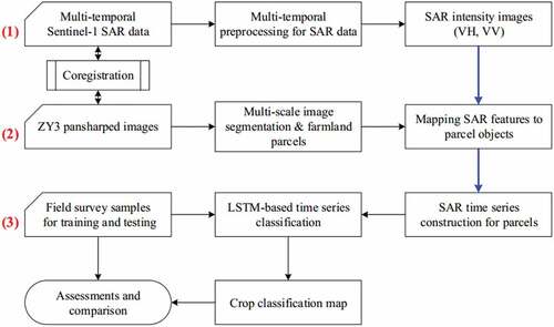
Before the main analysis, data pre-processing was conducted, which involved the fusion and mosaicking of optical images, geometrical registration for multi-source experimental data, and application of parameter settings. (1) Multi-temporal Sentinel-1A SAR data were processed to produce intensity images with VH and VV bands. (2) High-resolution optical images were first automatically segmented. Then, on the segmentation map, farmland parcels were identified and simplified (on their boundaries) to produce farmland parcel maps. (3) The multi-temporal SAR intensity images (with two intensity bands) were first overlaid onto the parcel map to construct parcel-based time series. Then, an LSTM-based classifier was applied to the time-series curves to produce a crop classification map of the same spatial resolution as that of the optical image.

2.1 Data processing

We used high-resolution ZY3 optical images which have one panchromatic band of a spatial resolution of 2.1 m and four multi-spectral bands (blue, green, red, near-infrared) of a spatial resolution of 5.8 m. The panchromatic band and multi-spectral bands were fused (using the Gram-Schmidt spectral sharpening algorithm via ENVI 5.1) to produce a pansharpened satellite image with a spatial resolution of 2.1 m, which was used to delineate the precise boundaries of farmland parcels. Due to their narrow swaths of 50 km, several ZY3 images with as close as possible acquisition times were registered and mosaiced to cover entire study areas.

Sentinel-1A SAR data with the interferometric wide swath (with a swath of 250 km and a spatial resolution of 5 m × 20 m) image mode were employed to construct time-series data. They are comprised of a VH polarization and a VV polarization in C band, with a 12-day repeat cycle. In this study, we collected all available Sentinel-1A data (distributed as single-look complex (SLC) product) during crop growing seasons from European Space Agency. In SARscape 5.3, Sentinel-1A SAR data were processed via multilooking, speckle filtering, geocoding and radiometric calibration, and geometric registration. First, the multilooking operation was applied to Sentinel-1A SLC products to generate intensity images of a VH band and a VV band. Second, a Lee filter with a 3 × 3 window size was performed on the intensity images to reduce speckle noise. Third, the image was geocoded using the shuttle radar topography mission (SRTM) DEM with a 90 m spatial resolution, and its digital number value was converted to a decibel (dB) scale backscatter coefficient. Finally, all intensity images were clipped and geometrically rectified to the Google satellite map using 9 manually selected ground control points. With these, multi-temporal intensity SAR images with a spatial resolution of 20 m were obtained, in which each pixel took a VH intensity value and a VV intensity value. Further, an intensity ratio (VH/VV) band could be produced and added into SAR data, which would be used as an additional variable for time-series analysis.

For the coregistration of experimental data (including optical images and SAR data), Google satellite map tiles (with a spatial resolution of 1.2 m) taken from Google’s Tile Map Service (TMS) were mosaiced to produce a satellite map covering the study areas. All experimental data were geometrically matched to the Google satellite map. Nine ground control points (manually selected from Google satellite map) for each ZY3 optical image and a polynomial model with 2 degrees (in ENVI 5.1) were used to geometrically correct the ZY3 image to the Google satellite map. Since the spatial extent of Sentinel-1A scenes is much larger than that of the study area, sub data covering the study area were clipped. Then, sub SAR data were geometrically corrected to the Google satellite map using a procedure similar to that employed for ZY3 images. Registration errors were amounted to less than 0.5 pixels at both the ZY3 and SAR spatial resolutions.

2.2 Farmland parcel extraction

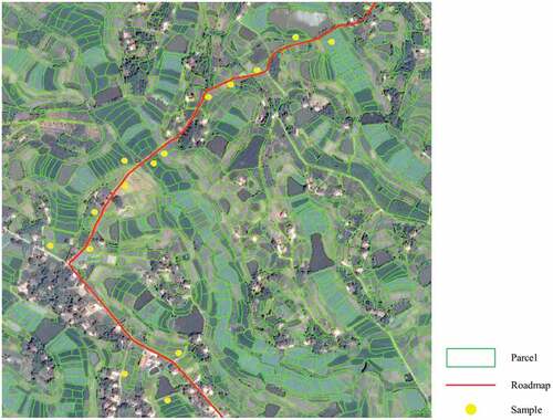
The adaptive multi-scale segmentation (AMS) method (Zhou, Li, et al., 2017), automatic identification, and manual correction were used to extract farmland parcels from the ZY3 pan-sharpened image. First, the AMS method was applied to the ZY3 image to produce a segmentation map of the whole study area with its default parameter settings. Second, with spectral features of the optical images, a two-class (one is crop parcel, the other is no-crop parcel) support vector machine classifier available through the scikit-learn package (Pedregosa, Gramfort, and Michel et al. 2013) was applied to the segmentation map to identify farmland parcels from segmentation objects. Then, interpretation experts further checked and corrected objects attributes to produce a farmland parcel map. Third, the boundaries of farmland parcels were further corrected and simplified to follow the edges of ground objects in the ZY3 image. The final farmland parcel map is presented in Figure 2, in which each parcel was used as a basic element for time time-series analysis.

Figure 2. Farmland parcels and field survey samples for crop classification.

Note that ZY3 optical images were used to delineate the precise parcels in our study. In practice, other available high-resolution images can also be employed (e.g., SPOT, QuickBird, GeoEye, WorldView, GF1 and GF2 satellite images) in consideration of the spatial resolution of images and the practical areas of fields.

2.3 Parcel-based time series construction

The processed multi-temporal SAR intensity images (Subsection 2.1) were overlaid onto the farmland parcel map (Subsection 2.2) to construct time series for each parcel. In SAR intensity images, pixels within the polygon of a farmland parcel were first searched. Then, the mean VH intensity value of these pixels was assigned to parcels as a VH feature, as was done for the VV intensity and the VH/VV ratio. Finally, three multi-temporal SAR intensity curves (VH intensity, VV intensity and VH/VV ratio) were constructed for each parcel.

SAR data are affected little from clouds and shadows, but data missing occasionally occurs. For example, the Sentinel-1A SLC product in DOY 166 (between 154 and 178 in Table 1) is not available from the European Space Agency. In this study, the type of data missing was considered as a system error for the time series analysis and was simply restored and assigned the mean intensity of the previous (DOY 154) and subsequent time (DOY 178).

Table 1. Sentinel-1 SAR data list used in this study (the data between DOY 154 and DOY 178 is missing).

Path/Frame	Day of Year	Path/Frame	Day of Year	Path/Frame	Day of Year	Path/Frame	Day of Year
11/94	−2(2016)	11/94	10	11/94	22	11/94	34
11/94	46	11/94	58	11/91	70	11/91	82
11/91	94	11/91	106	11/91	118	11/91	130
11/91	142	11/91	154	11/91	178	11/91	190
11/91	202	11/91	214	11/91	226	11/91	238
11/91	250	11/91	262	11/91	274	11/91	286
11/91	298	11/91	310	11/91	322	11/91	334
11/91	346	11/91	358	11/91	370(2018)

2.4 LSTM model for multivariate time series classification

1) Sample augmentation for classification

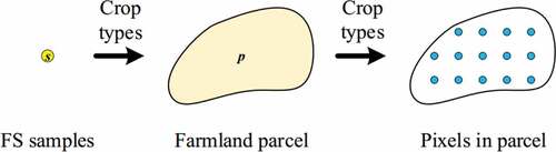
More samples are needed to train a deep learning model (such as LSTM) (Lecun, Bengio, and Hinton 2015) than that to train traditional machine learning algorithms such as the support vector machine (SVM) and random forest (RF) (Zhang, Zhang, and Du 2016; Ball, Anderson, and Chan 2017). However, in practice, there are limited field-survey (FS) samples, and collecting a volume of field samples would require the use of more manpower, financial resources and time. This constitutes a major disadvantage of deep learning algorithms used in remote sensing applications. In our experiments, a limited number of field-survey samples are insufficient for training the deep learning model. Thus, pixels within a parcel were used for sample augmentation to enhance the stability and generalization of the classifier (Dyk and Meng 2001; Ding, Chen, and Liu et al. 2016).

As is shown in Figure 3, a FS sample spot s was first overlaid onto the farmland parcel map while assigning its crop types (in three surveys) to the parcel p containing s. Then, each pixel (with its VH, VV, and ratio values) within the parcel p was assigned the crop types of parcel p and was independently utilized as a sample. As a result, much more pixel samples (than parcel samples) with time-series curves and crop types were obtained for the LSTM model. Finally, a k-fold cross validation was employed to divide these pixels into training samples and validation samples. To reduce the correlation between pixels within a farmland parcel and to avoid overfitting classifiers the division of folds were conducted at the parcel level, rather than at the pixel level so that pixels from a given parcel would not belong to different folds.

Figure 3. Sample augmentation for LSTM-based classification.

2) LSTM model for classification

Keras is a high-level framework used to build and train deep learning models that can run on top of TensorFlow, Microsoft Cognitive Toolkit, or Theano. Designed to enable fast experimentation with deep neural networks, it is being user-friendly, modular, and extensible for fast prototyping, advanced research, and production (Chollet 2017). In this study, a stacked LSTM model (Greff et al. 2017; Sun et al. 2017; Ienco, et al., 2017) built on the Keras framework was employed to construct a crop classifier. In this LSTM network (as shown in Figure 4), the multiple normalized (using the minmax normalization method with the minimum and maximum values from all time-series curves of the corresponding feature) time-series curves (such as the VH intensity) of samples were taken as the input (the time-series step of input is equal to the number of observation times, and the size of input is equal to the number of variables), and the output crop type was encoded via one-hot encoding, a common technique to categorical classification in machine learning (Rodríguez et al. 2018). Then, four LSTM layers with 36 hidden neurons (this is the optimal value in this study, which was discussed in Subsection 3.4) were stacked to transfer raw time-series curves into high-level features. Then, a dense layer was employed to fully connect the high-level features to crop categories. Finally, a Softmax activation function output the probabilities of crop types to produce crop classification maps.

Figure 4. Network structure of the LSTM-based classifier used for time series analysis.

While other configurations of the LSTM model in numbers of hidden neurons and different activation functions were tested (Subsection 3.4), the above configuration was found to achieve more stable and better performance in our cases.

2.5 Performance evaluation

Based on the confusion matrix (Foody 2002) derived by comparing classified results to the test samples parcel by parcel, user accuracy (UA), producer accuracy (PA), overall accuracy (OA), kappa coefficient and F1 measure values were calculated and used to evaluate the accuracy of crop classification. The OA is computed by dividing all correctly classified parcels by the entire validation dataset. The kappa is computed to determine whether the values in an error matrix are significantly better than the values of a random assignment. Additionally, F1 = 2× UA×PA/(UA+PA), is the harmonic mean of the producer and user accuracy. The F1 measure ranges from 0 to 1. A large F1 measure denotes good results and vice versa.

3. Experiments and discussion

Using ZY3 optical images and Sentinel-1A SAR data, experiments were carried out to test the performance of the proposed method. We compared the proposed approach to the traditional classification method (including an SVM classifier and an RF classifier). Accuracy evaluations were conducted on the parcel-based classification results, to discuss the improvement of the LSTM-based classification over the traditional classifications, VH intensity change during crop calendars, and parameter settings of the LSTM-based classifier.

3.1 Study area and dataset

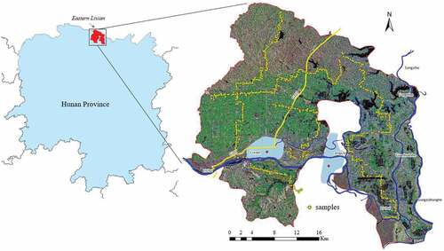
The first study area is located in the northern region of Hunan Province in China with central coordinates of 111°50ʹ E and 29°43ʹ N (Figure 5). The study area, covering a total area of 1210 km², is characterized by a subtropical humid monsoon climate with an annual average temperature of 16.7°C and abundant rainfall levels of 1200 mm to 1900 mm. These climatic conditions are suitable for rice, cotton and rape crop growth. According to the planting patterns presented in Figure 7, farming types can be classified into (single season) rice, double (season) rice, rice-rape, rape-rice, rape-rice-rape, rice-cotton, and other crops configurations, which are also the crop types used for classification in this study. “-” denotes crop rotation employed in sequenced seasons. Single season rice is planted once in a growing season, which lasts from May to October. Double season rice is planted twice during a growth season. First season rice (early rice) is transplanted in mid-April and harvested in mid-July, and second season rice (late rice) is planted soon after the harvest of first season rice and harvested in late October. Cotton lasts from May to October. Rape is planted in late October and harvested in mid-May of the following year.

Figure 5. The study area in northern Hunan Province, China. The right-hand section provides an overview of the SAR data (R: 23 May 2017 VH polarization, G: 26 October 2017 VH polarization, B: 3 August 2017 VV polarization), roadmaps and sample spots of the field survey.

Two ZY3 images acquired in May 2017 and two ZY3 images acquired in Oct 2017 were used to produce a mosaiced satellite map for delineating the precise boundaries of farmland parcels. In total, 31 Sentinel-1A SLC products from 30 December 2016 to 6 January 2018 were acquired to construct multi-temporal features of farmland parcels as shown in Table 1.

For supervised crop classification and accuracy assessments, three repetitive field surveys were conducted in May, August and November of 2017. The survey roadmap and sample spots are presented in Figure 5. To facilitate the field surveys, samples were distributed along roads. In surveys, a handheld GPS locator (with a precise point positioning precision level of 3.0 m) was used to record geographic position (in the same geographic coordinate system as the Google satellite map, WGS84) of samples. For each farmland parcel sampled, the crop type was recorded three times so that the three surveys fully recorded all potential crop types and rotations in one year. There were more than 1000 parcel samples collected, recording their geographic positions and crop types in three surveys. Though sample augmentation in Subsection 2.4, approximately 7000 pixel samples were obtained for classification.

3.2 Experimental setting

1) Classifiers for comparison: Two traditional classifiers were used for comparisons: an SVM classifier with a radial basis function kernel and an RF classifier. The GridSearchCV function with its default parameters (implemented in the scikit-learn package (Pedregosa, Gramfort, and Michel et al. 2013)) was employed to determine optimal parameters for the SVM (including kernel coefficient (“gamma”) and penalty parameter (“C”) of the error term) and RF classifiers (including the number of trees for the forest (“n_estimators”), the maximum tree depth (“max_depth”), and the number of features to consider when looking for the best split (“max_features”)). The final parameters of the SVM classifier were set to 2 for “C” and to 0.02 for “gamma” and those of the RF classifier were set to 120 for “n_estimators,” to 18 for “max_depth,” and to 36 for “max_features.”

2) Samples for classification: Sample augmentation produced approximately 7000 pixel samples to train and validate classifiers. For a 5-fold cross validation, 5600 samples were randomly selected for training, and the remaining 1400 were for validation, which was repeated 5 times.

3) Features for classification: The time-series curves were entered into the LSTM-based classifier. In the SVM and RF classifier, the VH and VV intensities of each period of time series were taken as independent features.

4) Other parameters: The number of farmland parcels considered was recorded as approximately 390,000.

3.3 Classification results

The crop classification map with a spatial resolution of 2.1 m and some typical sites produced by the proposed LSTM-based method are presented in Figures 6 and 7 (SAR data showed with the same colour combinations as those used in Figure 5).

Figure 6. Results of parcel-based crop classification for Hunan using the proposed method.

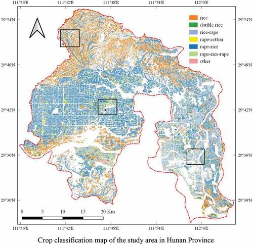
Figure 7. Local details of parcel-based crop classification for Hunan using the proposed method.

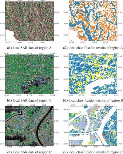
Limits to the manual interpretation of multi-temporal SAR data make it difficult to qualitatively evaluate classification performance by visual interpretation. However, overall performance can be assessed for some local areas. “Rice” is mainly distributed on sloped fields of hilly areas (in the north of the study area and not convenient for cultivation) (as shown in Figure 7 a2)) and across the suburbs around cities (as farmers have access to more means to make money, they are not actively engaged in farming). “Rape-rice” crops dominate river valleys in the north and plains in the midwest (as shown in Figure 7 b2)), and “rice-rape” and “rape-rice-rape” crops are mainly planted in the eastern region of study area with plentiful surface water reserves (the west branch of the Songzi River flows through this area) (as shown in Figure 7 c2)). This is also in line with water demands for rice growth. Since the study area is located in the northernmost area of double season rice growing regions, farmland parcels of “double rice” were sporadically distributed along rivers.

3.4 Evaluation and discussion

1) LSTM-based classifier vs. traditional classifiers (SVM and RF)

For comparisons, SVM and RF classifiers were applied to the parcel map to produce crop classification maps. We summarized the classification accuracies (including UA, PA and F1 scores for each crop type and OA and kappa scores for the whole map) derived from SVM-, RF- and LSTM-based classifiers with the VH and VV time series, as presented in Table 2.

Table 2. Comparison of overall accuracy, kappa coefficient and F1 measure values conducted using the SVM-, RF-, and LSTM-based classifiers for Hunan.

	SVM			RF			LSTM
crops	UA(%)	PA(%)	F1	UA(%)	PA(%)	F1	UA(%)	PA(%)	F1
rice	76.53	79.35	77.91	65.31	69.63	67.29	80.64	81.59	81.11
double rice	72.71	75.48	74.07	77.68	79.26	78.46	82.76	83.92	83.34
rice-rape	79.82	82.99	81.37	80.78	82.56	81.66	86.82	86.74	86.78
rape-cotton	76.63	74.95	75.78	83.82	85.43	84.62	81.42	83.23	82.32
rape-rice	74.12	77.70	75.87	74.62	75.14	74.88	84.57	85.76	85.16
rape-rice-rape	73.71	72.40	73.05	78.63	80.39	79.50	86.71	88.12	87.52
other	68.76	72.19	70.43	69.94	72.54	71.22	77.15	79.38	78.25
OA	75.50			76.82			83.67
kappa	71.79			73.58			80.91

It is clear that the LSTM-based classifier substantially outperformed the SVM and RF classifiers in UA, PA and F1 values for each class and in OA and kappa values for the whole classification map (improvements of approximate 8.0% and 7.0% in OA values, respectively). The SVM classifier, RF classifier and LSTM-based classifier achieved the highest F1 scores for “rice-rape,” “rape-cotton” and “rape-rice-rape” crops, respectively. Because the “other” type may include a combination of multiple unspecified crops, it achieved the poorest performance of all three classifiers. Let us take a closer look at the F1 scores of the LSTM-based classification. “Rape-rice-rape” crops generated the highest scores followed by “rape-rice” and “rice-rape” crops. The remaining crops generated lower scores. From a crop phenology perspective, it makes sense that rice and rape crops were planted in paddy fields and dry areas, respectively. Thus, “rape-rice-rape,” “rape-rice” and “rice-rape” crops present more evident and drastic changes (than other crops) in SAR intensity values. These changes are captured by the LSTM network and are represented as more salient time-series features, resulting in more precise classifications. The SVM and RF classifiers failed to capture these important features.

2) VH intensity time series vs. a crop calendar

On the classification map of the proposed method, for each crop type 200 parcels were randomly selected to calculate their mean time-series curves (only the VH intensity was analysed). We compared these time-series curves of crop types with the crop calendar for the study area, as presented in Figure 8. In the crop calendar, line segments represent crop growth cycles (e.g., first season rice of double rice crops is planted in April and is harvested in July), and the colours indicate crop types (brow line). We tried to determine the relationship between the change of VH intensity and the stages (planting, growth, maturity and harvesting) of crop cycles.

Figure 8. VH intensity time-series curves for crops (the upper section) and their corresponding crop calendars (the lower section) for Hunan.

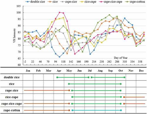
For “double rice” crops, first season crops (early rice) were transplanted in mid-April and harvested in mid-July, and the second round crops (late rice) were planted soon after and harvested in late October. Corresponding to the time-series curve, the VH intensity value dropped rapidly from mid-March to the end of April. During this period, fields were covered with water for subsequent rice transplanting, resulting in lower intensity value (backscattering coefficient) on SAR data. Then, the VH intensity rose rapidly and reached a peak in mid-June, as the rice grew. The VH intensity value remained at a peak until rice maturity was reached in mid-July. Then, the harvest of the first season and water storage for the second season lowered intensities. Again, the time-series curve reflects rapid growth (to the end of August), maturity, and harvesting (in late October) for the second season. The VH intensity time series for “single rice” crops are similar to that for the first season of “double rice” crops, but with crop growth occurring later (in mid-May) and with a longer crop cycle involved (to mid-October). For “rape-rice-rape” crops, the first rape crops were planted in the previous year. When temperatures increased at the end of February, as rape crop grew, the VH intensity rose rapidly and reached a peak between the end of April and beginning of May. Then, rape harvesting (in late May) and water storage (in early June) for the rice resulted in the lower intensities. Again, similar to what was observed in the second season of “double rice” crop growth, the growth, maturity and harvesting (in late October) of the rice resulted in a change in the VH intensity values. Because rape is a dryland crop with slow growth rates in the winter, VH intensity was maintained. For “rape-cotton” crops the VH intensity curve followed a similar pattern as the first “rape-rice-rape” crops. After rape harvesting (in late May), the VH intensity curve completed a cotton cycle with crop growth (from June to the end of August) increasing the VH intensity value and with crop harvesting (in Mid-October) decreasing the VH intensity value.

3) Univariable vs. multivariate time series

To further test the LSTM-based classifier with multiple variables, we conducted a series LSTM-based classifications (with other setting constant) using (1) three time-series variables (VH intensity, VV intensity, and the ratio of VH to VV), (2) two time-series variables (VH intensity and VV intensity), (3) univariable time-series variable VH, and (4) univariable time-series variable VV, respectively. The final classification accuracies are presented in Table 3.

Table 3. Classification performance using multivariate and univariable time series for Hunan.

		Variables
classifier	Accuracy(%)	VH+VV+R	VH+VV	VH	VV
SVM	OA	75.38	75.50	71.68	72.94
	Kappa	72.07	71.79	66.83	68.96
RF	OA	77.37	76.82	74.09	72.41
	Kappa	73.13	73.58	70.57	69.12
LSTM	OA	84.21	83.67	78.43	77.06
	Kappa	81.40	80.91	74.36	72.64

Overall, classifications using the VH+VV+R and VH+VV variables achieved better performance than those using the VH and VV variables for the three classifiers (especially for the LSTM-based classifier). This was expected, as the use of more features should generally improve classifications. Further, promotions for the LSTM-based classifier (approximately 5.0% for OA) were much greater than those of the SVM (approximately 2.0% for OA) and RF classifiers (approximately 3.0% for OA). We believe that the LSTM model can use deeper networks to learn the intrinsic features of time-series curves and mutual features between time-series curves relative to traditional classifiers. Furthermore, more accurate results were achieved when using VH+VV+R variables than VH+VV variables, but the difference is not significant (less than 1.0%). As observed from the spectral bands of optical images, VH and VV intensity values reveal the interaction of microwaves and crops, in two polarization modes. Thus, more polarization modes would improve capacities to distinguish between different crops, which is consistent with the results of previous studies (Jia et al. 2012; Parihar et al. 2014; Zhou, Pan, et al., 2017). However, as a derived feature of VH and VV, R is superfluous in theory, and cannot be used to improve classification accuracies.

4) Classification performance with the number of hidden neurons

As an important parameter of neural networks, the number of neurons in a hidden layer has a considerable influence on the classification performance of LSTM models. Thus, a series of experiments that involved increasing the number (from 2 to 40, at intervals of 2) of neurons in hidden layers (with other parameter settings constant) was carried out to determine a suitable number of hidden neurons to use for crop classification. In each experiment with a special number of neurons, we measured the OA value of classification results, as shown in Figure 9.

Figure 9. Classification performance as a function of the number of neurons in hidden layers.

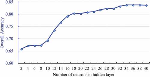
When using fewer neurons (2 ~ 8), the OAs (less than 68.0%) of classification maps were stable and lower than those of the traditional classifiers, showing that hidden layers with too few neurons cannot learn useful dependencies from time-series observations. When the number of hidden neurons increased from 10 to 20, classification performance rose rapidly to 80.02%, indicating that useful features had been learned. When the number increased from 22 to 34, the performance continued to improve at minor increments. When the number exceeded 34, performance reached a stable value with an OA of 83.67%. We thus set the number of neurons in the hidden layer as 36 for our experiment of the study area.

5) Classification performance as a function of time series

Crops follow various growth patterns related to sowing, harvesting and growing periods. The use of more crop period measurement (especially in critical growth periods) should improve the performance of crop classifications. Thus, a group of experiments was carried out to test classification accuracies along with more time-series periods. In the first experiment, we used SAR data from the first period (DOY −2), in the second experiment, we used SAR data from the first two period (DOY −2 and DOY 10), and so on. Then, we measured overall accuracies of these experiments, as presented in Figure 10.

Figure 10. Classification performance as a function of time series.

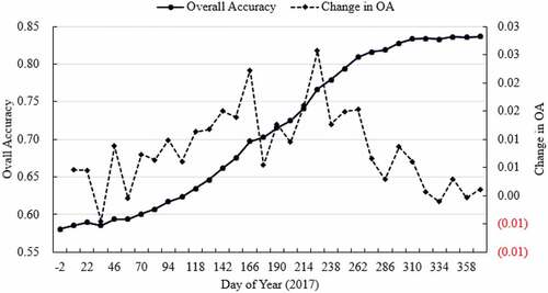
Increases (change in OA) in OA values were less significant at the beginning of the year (before DOY 100) and then increased in the middle of year (DOY 100 to DOY 260), after which they decreased once again (after DOY 260). More significant increases occurred from DOY 100 to DOY 260. This period reflects the crop growing season, in which more evident changes in SAR intensities appear. These changes were captured with the LSTM-based classifier to improve classification. A sharp drop occurred at DOY 178. Because the intensity measured for DOY 166 is the mean value of those of DOY 154 and DOY 178, DOY 178 is superfluous in theory when we already include DOY 154 and DOY 166 in the time series. Thus, the addition of DOY 178 to the time series failed to considerably improve accuracy values.

3.5 More experiments

To further test the proposed method for other study area, we carried out another experiment on the central area of Guizhou Province in China, following the same procedures. The area is a part of the Yunnan-Guizhou Plateau with altitudes of 850 m to 1300 m. Due to shorter sunshine periods (less than 1400 hours/year) and lower annual mean temperatures, fields were covered with annual crops (including rice and maize), perennial sciophilous fruits (including Roxburgh rose and kiwifruit) and diverse vegetables (collectively called other types). We collected a ZY3 images (acquired on April 2018), 25 Sentinel-1A SLC products (from Jan. 9 to Nov. 5 with a data missing for Aug. 13), and approximately 3400 field survey samples in 2018 for crop classification. The final classification results (240,000 parcels) are presented in Figures 11 and 12, with accuracy evaluations given in Table 4 in relation to the SVM and RF classifier results. The SAR data was presented in colour combinations relating to 21 May 2018 VH polarization (as R), 30 September 2018 VH polarization (as G), and 21 May 2018 VV polarization (as B).

Table 4. Comparison of overall accuracy values for Guizhou using the SVM-, RF-, and LSTM-based classifiers.

classifier	SVM	RF	LSTM
OA (%)	72.64	74.19	80.71

Figure 11. Results of the parcel-based crop classification for Guizhou using the proposed method.

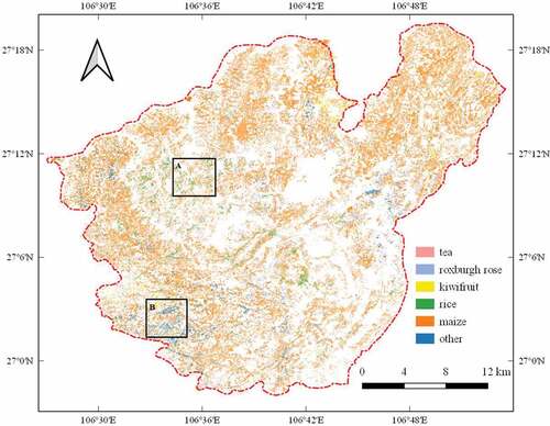
Figure 12. Local details of the parcel-based crop classification for Guizhou using the proposed method.

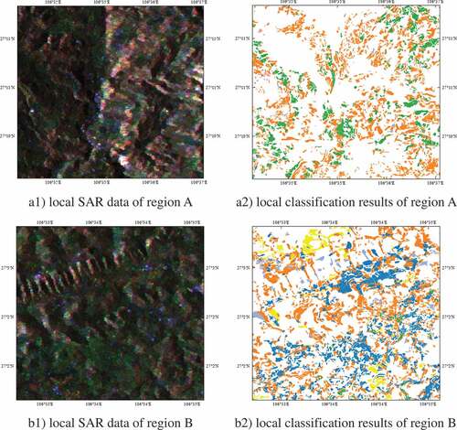
Overall, the spatial distribution of crops was constrained by natural conditions and was affected by economic factors. “Rice” crops were mainly planted in terraced fields (local region A in Figure 12), in which water can irrigate each terrace from top to bottom, under the force of gravity. Local region B includes many small plains suitable for planting cash crops. It is positioned close to Guiyang, the capital of Guizhou Province. Thus, “other” crops (various vegetables) are the main crops grown here.

According to these accuracy evaluations, experiments conducted in Guizhou performed less effectively than those in Hunan, because complex topographic features generated no-signal areas in SAR data and time series are not complete for crop cycles. However, the LSTM-based classifier achieved an OA score 80.71%, which is higher than the value of 72.64% found for the SVM classifier and the value of 74.19% found for the RF classifier.

4. Conclusion

Crop classification using multi-temporal SAR data is essential to precision agriculture in southern China. We have proposed an LSTM-based multi-variable time-series analysis method for parcel-scale crop classification, based on the spatial-temporal incorporation of high-resolution optical images and multi-temporal SAR data. The method was applied to produce a crop classification map from datasets of ZY3 optical images and Sentinel-1A SAR data for Hunan and Guizhou in China. The classification results, showing a promotion value of greater than 5.0% in overall accuracy relative to traditional methods, demonstrates the effectiveness of the proposed method for parcel-based crop classification in southern China. The approach can serve as a new approach to precise crop classification for cloudy and rainy regions.

Despite these encouraging results, more work is needed to further explore the use of deep learning for time-series analysis such as, 1) extracting more features (in addition to intensities, such as textures, correlation coefficients, and some learned features using deep learning techniques) from SAR data to construct more time-series variables to improve the classification performance, 2) augmenting data (e.g., adding random or Gaussian noise, interpolating, and random frequency filtering) to produce more samples for training and validating LSTM models, 3) using available middle-resolution optical images (e.g., Sentinel-2 and GF1 images) to enhance time series analysis and developing corresponding deep learning models for the multi-source irregular time-series analysis approach, and 4) establishing meaningful correspondence from feature spaces learned using LSTM models to measure crop growth stages quantificationally.

Correction Statement

This article has been republished with minor changes. These changes do not impact the academic content of the article.

Disclosure statement

No potential conflict of interest was reported by the authors.

Additional information

Funding

This work was supported in part by the National Key Research and Development Program under Grant [2017YFB0503600]; the National Natural Science Foundation of China under Grant No. [41501453 and 41631179]; the Fundamental Research Funds for the Central Universities under Grant No. [2019B17114]; the Opening Foundation of Key Lab of Spatial Data Mining & Information Sharing, Ministry of Education (Fuzhou University) under Grant No. [2019LSDMIS04].

References

- Andra Baduge A. W, Hanshel M., Hobbs S., Buehler S. A., Ekman J., Lehrbass B. 2016 Seasonal variation of coherence in SAR interferograms in Kiruna, Northern Sweden. International Journal of Remote Sensing. 37 (2):370–87.
- Ball, J. E., D. T. Anderson, and C. S. Chan. 2017. “A Comprehensive Survey of Deep Learning in Remote Sensing: Theories, Tools and Challenges for the Community.” Journal of Applied Remote Sensing 11 (4). doi:10.1117/1.JRS.11.042609.
- Ban, Y., and A. Jacob. 2013. “Object-Based Fusion of Multitemporal Multiangle ENVISAT ASAR and HJ-1B Multispectral Data for Urban Land-Cover Mapping.” IEEE Transactions on Geoscience & Remote Sensing 51 (4): 1998–2006. doi:10.1109/TGRS.2012.2236560.
- Bargiel, D. 2017. “A New Method for Crop Classification Combining Time Series of Radar Images and Crop Phenology Information.” Remote Sensing of Environment 198: 369–383. doi:10.1016/j.rse.2017.06.022.
- Chollet, F. 2017. Deep Learning with Python. Grand Forks, ND: Manning Publications .
- Ding J, Chen B, Liu H and Mengyuan H. 2016. “Convolutional Neural Network with Data Augmentation for SAR Target Recognition.” IEEE Geoscience & Remote Sensing Letters 13 (3): 364–368.
- Dong, J., X. Xiao, B. Chen, N. Torbick, C. Jin, G. Zhang, and C. Biradar. 2013. “Mapping Deciduous Rubber Plantations through Integration of PALSAR and Multi-temporal Landsat Imagery.” Remote Sensing of Environment 134 (134): 392–402. doi:10.1016/j.rse.2013.03.014.
- Dusseux, P., T. Corpetti, L. Hubertmoy, and S. Corgne. 2014. “Combined Use of Multi-Temporal Optical and Radar Satellite Images for Grassland Monitoring.” Remote Sensing 6 (7): 6163–6182. doi:10.3390/rs6076163.
- Dyk, D. A. V., and X. L. Meng. 2001. “The Art of Data Augmentation.” Journal of Computational & Graphical Statistics 10 (1): 1–50. doi:10.1198/10618600152418584.
- Foody, G. M. 2002. “Status of Land Cover Classification Accuracy Assessment.” Remote Sensing of Environment 80 (1): 185–201. doi:10.1016/S0034-4257(01)00295-4.
- Gao, F., M. C. Anderson, X. Zhang, Z. Yang, J. G. Alfieri, W. P. Kustas, R. Mueller, D. M. Johnson, and J. H. Prueger. 2017. “Toward Mapping Crop Progress at Field Scales through Fusion of Landsat and MODIS Imagery.” Remote Sensing of Environment 188: 9–25. doi:10.1016/j.rse.2016.11.004.
- Greff, K., R. K. Srivastava, J. Koutnik, B. R. Steunebrink, and J. Schmidhuber. 2017. “LSTM: A Search Space Odyssey.” IEEE Transactions on Neural Networks & Learning Systems 28 (10): 2222–2232. doi:10.1109/TNNLS.2016.2582924.
- Gumma M K, Thenkabail P S, Deevi K C, Mohammed I A, Teluguntla P, Oliphant A, Xiong J, Aye T, Whitbread A M. 2018. “Mapping Cropland Fallow Areas in Myanmar to scale up sustainable intensification of pulse crops in the Farming System[J].” Giscience & Remote Sensing, 55(6): 926–949.
- Ienco D, Gaetano R, Dupaquier C and Maurel P. 2017. “Land Cover Classification via Multitemporal Spatial Data by Deep Recurrent Neural Networks.” IEEE Geoscience & Remote Sensing Letters PP (99): 1–5.
- Inglada, J., A. Vincent, M. Arias, and C. Marais-Sicre. 2016. “Improved Early Crop Type Identification by Joint Use of High Temporal Resolution SAR and Optical Image Time Series.” Remote Sensing 8 (5): 362. doi:10.3390/rs8050362.
- Jia, K., Q. Li, Y. Tian, B. Wu, F. Zhang, and J. Meng. 2012. “Crop Classification Using Multi-configuration SAR Data in the North China Plain.” International Journal of Remote Sensing 33 (1): 170–183. doi:10.1080/01431161.2011.587844.
- Jiao, X., J. M. Kovacs, J. Shang, H. McNairn, D. Walters, B. Ma, and X. Geng. 2014. “Object-oriented Crop Mapping and Monitoring Using Multi-temporal Polarimetric RADARSAT-2 Data.” Isprs Journal of Photogrammetry & Remote Sensing 96 (96): 38–46. doi:10.1016/j.isprsjprs.2014.06.014.
- Joshi, N., M. Baumann, A. Ehammer, R. Fensholt, K. Grogan, P. Hostert, M. Jepsen, et al. 2016. “A Review of the Application of Optical and Radar Remote Sensing Data Fusion to Land Use Mapping and Monitoring.” Remote Sensing 8 (1): 70. doi:10.3390/rs8010070.
- Kim, M., J. Ko, S. Jeong, J.-M. Yeom, and H.-O. Kim. 2018. “Monitoring Canopy Growth and Grain Yield of Paddy Rice in South Korea by Using the GRAMI Model and High Spatial Resolution Imagery.” Giscience & Remote Sensing 54 (4): 534–551. doi:10.1080/15481603.2017.1291783.
- Kussul N, Lavreniuk M, Skakun S, Lavreniuk M, and Shelestov, A. Y. 2017. “Deep Learning Classification of Land Cover and Crop Types Using Remote Sensing Data.” IEEE Geoscience & Remote Sensing Letters PP (99): 1–5.
- Larrañaga, A., J. ÁlvarezMozos, and L. Albizua. 2011. “Crop Classification in Rain-fed and Irrigated Agricultural Areas Using Landsat TM and ALOS/PALSAR Data.” Canadian Journal of Remote Sensing 37 (1): 157–170. doi:10.5589/m11-022.
- Lecun, Y., Y. Bengio, and G. Hinton. 2015. “Deep Learning.” Nature 521 (7553): 436. doi:10.1038/nature14539.
- Mandal D, Kumar V, Bhattacharya A, and Rao Y. “Monitoring Rice Crop Using Time Series Sentinel-1 Data in Google Earth Engine Platform.” Asian Conference on Remote Sensing,38th Asian Conference on Remote Sensing, ACRS 2017, At New Delhi, India.
- McNairn, H., A. Kross, D. Lapen, R. Caves, and J. Shang. 2014. “Early Season Monitoring of Corn and Soybeans with TerraSAR-X and RADARSAT-2.” International Journal of Applied Earth Observation & Geoinformation 28 (5): 252–259. doi:10.1016/j.jag.2013.12.015.
- Olesk, A., J. Praks, O. Antropov, K. Zalite, T. Arumäe, and K. Voormansik. 2016. “Interferometric SAR Coherence Models for Characterization of Hemiboreal Forests Using TanDEM-X Data.” Remote Sensing 8 (9): 700. doi:10.3390/rs8090700.
- Onojeghuo, A. O., G. A. Blackburn, Q. Wang, P. M. Atkinson, D. Kindred, and Y. Miao. 2018. “Rice Crop Phenology Mapping at High Spatial and Temporal Resolution Using Downscaled MODIS Time-series.” Giscience & Remote Sensing. doi:10.1080/15481603.2018.1423725.
- Parihar, N., A. Das, V. S. Rathore, M. S. Nathawat, and S. Mohan. 2014. “Analysis of L-band SAR Backscatter and Coherence for Delineation of Land-use/land-cover.” International Journal of Remote Sensing 35 (18): 6781–6798. doi:10.1080/01431161.2014.965282.
- Park, S., J. Im, S. Park, C. Yoo, H. Han, and J. Rhee. 2018. “Classification and Mapping of Paddy Rice by Combining Landsat and SAR Time Series Data.” Remote Sensing 10 (3): 447. doi:10.3390/rs10030447.
- Pedregosa F., Varoquaux G., Gramfort A., Michel V., and Thirion B. 2013. “Scikit-learn: Machine Learning in Python.” Journal of Machine Learning Research 12 (10): 2825–2830.
- Reddy, D. S., and P. R. C. Prasad. 2018. “Prediction of Vegetation Dynamics Using NDVI Time Series Data and LSTM.” Modeling Earth Systems & Environment, no.4(1): 1–11.
- Rodríguez, P., M. A. Bautista, J. Gonzàlez, and S. Escalera. 2018. “Beyond One-hot Encoding: Lower Dimensional Target Embedding.” Image & Vision Computing 75: 21–31. doi:10.1016/j.imavis.2018.04.004.
- Shao, Y., X. Fan, H. Liu, J. Xiao, S. Ross, B. Brisco, R. Brown, and G. Staples. 2001. “Rice Monitoring and Production Estimation Using Multitemporal RADARSAT.” Remote Sensing of Environment 76 (3): 310–325. doi:10.1016/S0034-4257(00)00212-1.
- Silva, W. F., B. F. T. Rudorff, A. R. Formaggio, W. R. Paradella, and J. C. Mura. 2009. “Discrimination of Agricultural Crops in a Tropical Semi-arid Region of Brazil Based on L-band Polarimetric Airborne SAR Data.” Isprs Journal of Photogrammetry & Remote Sensing 64 (5): 458–463. doi:10.1016/j.isprsjprs.2008.07.005.
- Skakun, S., N. Kussul, A. Y. Shelestov, M. Lavreniuk, and O. Kussul. 2016. “Efficiency Assessment of Multitemporal C-Band Radarsat-2 Intensity and Landsat-8 Surface Reflectance Satellite Imagery for Crop Classification in Ukraine.” IEEE Journal of Selected Topics in Applied Earth Observations & Remote Sensing 9 (8): 3712–3719. doi:10.1109/JSTARS.2015.2454297.
- Skriver, H. 2012. “Crop Classification by Multitemporal C- and L-Band Single- and Dual-Polarization and Fully Polarimetric SAR.” IEEE Transactions on Geoscience & Remote Sensing 50 (6): 2138–2149. doi:10.1109/TGRS.2011.2172994.
- Su, T. 2017. “Efficient Paddy Field Mapping Using Landsat-8 Imagery and Object-Based Image Analysis Based on Advanced Fractel Net Evolution Approach.” Mapping Sciences & Remote Sensing 54 (3): 354–380. doi:10.1080/15481603.2016.1273438.
- Sun, X., T. Li, Q. Li, Y. Huang, and Y. Li. 2017. “Deep Belief Echo-state Network and Its Application to Time Series Prediction.” Knowledge-Based Systems. doi:10.1016/j.knosys.2017.05.022.
- Ulaby, F. T., R. K. Moore, and A. K. Fung. 1986. Microwave Remote Sensing: Active and Passive. Volume III: From Theory to Applications. Vol. 3. Dedham, MA: Artech House, Inc..
- Veloso, A., S. Mermoz, A. Bouvet, T. Le Toan, M. Planells, J.-F. Dejoux, and E. Ceschia. 2017. “Understanding the Temporal Behavior of Crops Using Sentinel-1 and Sentinel-2-like Data for Agricultural Applications.” Remote Sensing of Environment 199: 415–426. doi:10.1016/j.rse.2017.07.015.
- Wang, C., Q. Fan, Q. Li, W. M. SooHoo, and L. Lu. 2017. “Energy Crop Mapping with Enhanced TM/MODIS Time Series in the BCAP Agricultural Lands.” Isprs Journal of Photogrammetry & Remote Sensing 124: 133–143. doi:10.1016/j.isprsjprs.2016.12.002.
- Whelen, T., and P. Siqueira. 2018. “Time-series Classification of Sentinel-1 Agricultural Data over North Dakota.” Remote Sensing Letters 9 (5): 411–420. doi:10.1080/2150704X.2018.1430393.
- Yang, Y., Q. Huang, W. Wu, J. Luo, L. Gao, W. Dong, T. Wu, and X. Hu. 2017. “Geo-Parcel Based Crop Identification by Integrating High Spatial-Temporal Resolution Imagery from Multi-Source Satellite Data.” Remote Sensing 9 (12): 1298. doi:10.3390/rs9121298.
- Zeyada, H. H., M. M. Ezz, A. H. Nasr, M. Shokr, and H. M. Harb. 2016. “Evaluation of the Discrimination Capability of Full Polarimetric SAR Data for Crop Classification.” International Journal of Remote Sensing 37 (11): 2585–2603. doi:10.1080/01431161.2016.1182663.
- Zhang, H., Q. Li, J. Liu, J. Shang, X. Du, L. Zhao, N. Wang, and T. Dong. 2017. “Crop Classification and Acreage Estimation in North Korea Using Phenology Features.” Mapping Sciences & Remote Sensing 54 (3): 381–406. doi:10.1080/15481603.2016.1276255.
- Zhang, L., L. Zhang, and B. Du. 2016. “Deep Learning for Remote Sensing Data: A Technical Tutorial on the State of the Art.” IEEE Geoscience & Remote Sensing Magazine 4 (2): 22–40. doi:10.1109/MGRS.2016.2540798.
- Zhou T, Pan J, Zhang P, Wei S, and Han T. 2017. “Mapping Winter Wheat with Multi-Temporal SAR and Optical Images in an Urban Agricultural Region.” Sensors 17 (6): 1210. DOI:10.3390/s17050968.
- Zhou, Y., J. Li, L. Feng, X. Zhang, and X. Hu. 2017. “Adaptive Scale Selection for Multiscale Segmentation of Satellite Images.” IEEE Journal of Selected Topics in Applied Earth Observations & Remote Sensing 10 (8): 3641–3651. doi:10.1109/JSTARS.2017.2693993.