Spatio-Temporal Reconstruction of MODIS NDVI by Regional Land Surface Phenology and Harmonic Analysis of Time-Series

Abstract

Satellite-derived Normalized Difference Vegetation Index (NDVI) is frequently obstructed by adverse atmospheric components resulting in data gaps in time series. The harmonic analysis of time series (HANTS) algorithm is a widely used technique to reconstruct missing NDVI time series. However, due to restriction of HANTS to act within temporal dimension, its direct application is bound to endure practical problems in spatiotemporal reconstruction due to large data gaps. This study proposes Moving Offset Method (MOM), a novel prefilling method applied on NDVI time series prior to application of HANTS. MOM restores the missing NDVI time series by assuming that it tends to follow a reference pattern of land surface phenology (NDVI_ref). The NDVI_ref is prepared by using a recursive search and fill algorithm (SFA) for data availability without null values. It restores null values in NDVI_ref at a pixel by using coefficients of linear regression with NDVI_ref at another pixel having identical conditions. Finally, the prefilling is prior to application of HANTS. The proposed approach is demonstrated by using MODIS 16-daily time series data for Northeast India and Bhutan region which is covered with frequent seasonal clouds. Besides direct application of HANTS, it is also compared with similar approaches which includes prefilling by inverse distance weighted (IDW) and cubic spline, prior to application of HANTS. The fitting indicators, overall reconstruction error (ORE) and normalized noise related error (NNRE) are found to be best for proposed approach in spatiotemporal comparison. Also, restoration of seasonality trait the NDVI time series better in the proposed approach. This approach is concluded to be an enhancement for HANTS that could be helpful in improving quality of NDVI reconstruction for regions with frequent seasonal obstructions around the globe.

Keywords:

• time series reconstruction
• HANTS
• NDVI
• land surface phenology

1. Introduction

Satellite-derived Normalized Difference Vegetation Index (NDVI) has essential applications in modern terrestrial studies due to its proficiency to reveal vegetation strength. Its application extends to fields such as hydrology (Ahmed et al. 2017; Liu et al. 2015), hydrometeorology (Xiong and Qiu 2011; Carter et al. 2018; Joiner et al. 2018), agriculture (Panda, Ames, and Panigrahi 2010; Glennie and Anyamba 2018; Padhee et al. 2017), disaster management (Lin et al. 2004; Gandhi et al. 2015), and climate change (Kundu et al. 2018; Szabó et al. 2018). Hence, continuous spatiotemporal availability of high-quality NDVI is a necessity for time-series-based studies in these fields.

NDVI is computed as the normalized ratio of the difference in surface reflectance in near-infrared and red spectrum range to their sum (Tucker 1979). The reflectance channels measured by the satellite sensors in these spectrum ranges are obstructed by atmospheric components such as clouds, aerosol, fog, smoke, etc. So, it creates hindrance in obtaining continuous spatiotemporal NDVI (Carreiras et al. 2003; Kobayashi and Dy 2005). Justice et al. (1985) first identified that NDVI could misestimate the presence of vegetation by compositing different channels in numerous atmospheric conditions, which we know as “noise.” Holben (1986) was among one of the first studies which suggested suppressing defective NDVI values in the time series by maximum-value composite (MVC). In this procedure, NDVI was calculated from spectral channels with best pixel value within a period of time, e.g. NDVI MVC from NOAA/AVHRR, SPOT/VEGETATION, TERRA or AQUA/MODIS, etc. Besides suppressing noise, MVC products also reduce data gaps caused by cloud-contaminated pixels in NDVI time series (Jia et al. 2011). However, even after MVC procedure, both noise and data gaps in the time series are reported (Jönsson and Eklundh 2004; Chen et al. 2004; Ma and Veroustraete 2006; Ren et al. 2008; Geng et al. 2014). Subsequently, several methods have been developed to support time series analysis with NDVI continuity (Geng, Ma, and Wang 2016).

The popular reconstruction techniques used after MVC can be categorized into five groups according to their application methods:

1. Running filter techniques – Savitzky-Golay (SG) filtering (Savitzky and Golay 1964; Chen et al. 2004), the mean value iteration filter (MVI) (Ma and Veroustraete 2006), the changing-weight filter (CW) (Zhu et al. 2012);

2. Function fitting techniques – Fast Fourier transform and harmonic analysis of time series (FFT/HANTS) (Menenti et al. 1993; Verhoef, Menenti, and Azzali 1996; Roerink, Menenti, and Verhoef 2000), the double logistic function fitting (DL) (Fischer 1994; Beck et al. 2006), the temporal window operation (TWO) (Park, Tateishi, and Matsuoka 1999), the asymmetric Gaussian function fitting (AG) (Jönsson and Eklundh 2004);

3. Thresholding techniques – the Best index slope extraction (BISE) (Viovy, Arino, and Belward 1992), and the modified BISE (M-BISE) Lovell and Graetz 2001);

4. Hybrid techniques – data assimilation (Gu et al. 2009), iterative interpolation for data reconstruction (IDR) (Julien and Sobrino 2010);

5. Other techniques – wavelet transform (Lu et al. 2007), and the Whittaker smoother (WS) (Atzberger and Eilers 2011a, 2011b).

Most of these reconstruction techniques are highly dependent on the available data at a specific location. Hence, a major limitation arises with the possibility of insufficient observation frequency which can affect the quality of NDVI continuity in time series. There is a need to incorporate efficient methodologies to overcome this problem.

HANTS is a popular algorithm used worldwide and has been concluded as one of the finest reconstruction techniques (Zhou et al. 2016; Geng, Ma, and Wang 2016; Julien and Sobrino 2019). Application of HANTS on NDVI time series was first seen for Southern African and American Continents in the works of Verhoef, Menenti, and Azzali (1996). Roerink, Menenti, and Verhoef (2000) described the details on parameterization in HANTS algorithm by demonstrating its application on AVHRR 10-daily-NDVI MVC over Europe. This algorithm has been used for a variety of applications with the aim of consistent NDVI time series availability. It includes assessing the impacts of climate on vegetation (Roerink et al. 2003; Jiang et al. 2014), understanding land cover dynamics (Morton et al. 2006; Wen et al. 2010; Wang et al. 2014), and determination of vegetation-based biophysical variables (Wen and Su 2004; Gokmen et al. 2013; Li, Jia, and Zheng 2014; Li et al. 2018), etc. However, one of the major drawbacks of HANTS is its poor performance during large data gaps in the NDVI time series (Xu et al. 2015). The primary reason for this drawback is temporal-bound nature of HANTS algorithm. It is difficult to attain good performance for all possible combinations of gap solely by HANTS (Atzberger and Eilers 2011b). Therefore, prefilling the NDVI time series prior to application of HANTS has been addressed in limited recent studies, e.g. Temporal-Similarity-Statistics (TSS) by Jia et al. (2011) and spline by Liang et al. (2017). However, prefilling in these studies are either limited to temporal dependence or do not reflect the land surface phenology. Musial, Verstraete, and Gobron (2011) concluded that the optimal gap-filling approach for geophysical time series depends on the type and distribution of gaps. In the present study, spatiotemporal similarity statistics is anticipated to overcome the mentioned limitations.

Phenology is the timing of recurring biological events driven by biotic and abiotic forces (Liu et al. 2014). Land surface phenology deals with cyclic pattern of land surface vegetation and it is used as a key indicator of vegetation dynamics. Application of HANTS algorithm has enabled to understand the vegetation evolution and phenological characteristics in the last two decades (Jun, Zhongbo, and Yaoming 2009; Liu et al. 2014; Anav et al. 2018). The phenology of vegetation is largely associated with climate and terrain characteristics (Azzali and Menenti 2000; Chen 2017; Kiapasha et al. 2017). Moreover, vegetation in the same ecoregion faces similar climate and human conditions (Yang et al. 2017). Due to this reason, various classes of land-use/land-cover (LULC) are often classified by using land surface phenology (Friedl et al. 2002; Padhee et al. 2017). Therefore, we can draw that land surface phenology of a particular LULC is supposed to vary similarly to that of same LULC with identical conditions in same ecoregion. However, formerly the time series data of NDVI is used to delineate land surface phenology (Xiao et al. 2009). NDVI time series dataset reflects natural phenomena which is nonlinear (Verma and Dutta 2013) and usually is a resultant of components such as noise, inter-annual fluctuations, and long-term trends (de Beurs and Henebry 2005; Verbesselt et al. 2010). It means NDVI trajectory continuously tends to follow local phenology (phenology at a spatial location or pixel) and any deviation from it is due to noise, inter-annual fluctuations, and/or long-term trends. Since, there is a strong link between NDVI, local phenology and regional LULC, approaches involving spatiotemporal investigation of land surface phenology of LULC are expected to grasp essential evidences for missing NDVI in highly cloud-contaminated regions.

In this paper, shortcomings of HANTS due to variable and large data gaps in the time series is solved by prefilling the NDVI time series with a novel method called “Moving Offset Method (MOM)” prior to application of HANTS. MOM utilizes a reference phenology curve at a pixel (derived from NDVI time series at the same pixel) to predict missing values in NDVI time series as good as MVC. Deficiency of NDVI values in time series data at a pixel to derive reference phenology curve is confronted by an innovative recursive search and fill algorithm (SFA). The SFA uses spatiotemporal similarity of phenology between the data-deficient pixel and its most identical pixel of same LULC with a set of conditions. The Northeast India and Bhutan, a region frequently covered with clouds, was selected as the study area. The present work demonstrates spatiotemporal comparison between reconstructed NDVI time series by HANTS applied for original data and prefilled data by MOM. Since, many previous methods have used linear or spline interpolations (e.g. Chen et al. 2004; Julien and Sobrino 2010; Liang et al. 2017) as modes of interpolating missing values in NDVI time series, performance of MOM is also compared with inverse distance weight (IDW) and cubic spline as competent prefilling methods. The practical applicability of the proposed approach using MOM is concluded on the basis of spatiotemporal comparison of seasonality trait as well as fitting performance.

2. Materials and methods

2.1. Study area

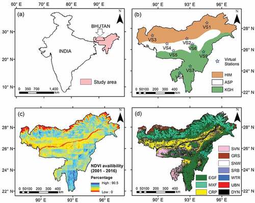
Northeast India is well known for frequently covered with clouds in monsoon season (Jain, Kumar, and Saharia 2013; Jaswal, Kore, and Singh 2017) due to which it is selected as the study area. It consists of three major ecoregions (Eastern Himalayas, Assam plains, and Khasi & Garo hills) as shown in Figure 1(b). The Bhutan country falls within the Eastern Himalayan ecoregion due to which it is also included in the study area (Figure 1).

Figure 1. (a) Location of the study area. (b) Ecoregions (HIM: Himalaya; ASP: Assam plains; KGH: Khasi & Garo hills) and virtual stations in the study area. (c) NDVI data availability (2001–2016) in the study area. (d) Land use/land cover (2001–2016) in the study area (EGF: Evergreen forest; MXF: Mixed forest; CRP: Cropland; SVN: Savanna; GRS: Grassland; SNW: Snow; SRB: Shrub land; WTR: Waterbody; UBN: Urban area; DYN: Dynamic LULC).

2.2. Data description

2.2.1. Normalized difference vegetation index

MODIS-NDVI is one of the widely used NDVI MVC products in research related to vegetation phenology (Beck et al. 2006; Bucha and Koren 2017; Testa et al. 2018). The NDVI 16-daily MVC product from Terra-MODIS (MOD13A1 v006) at 500 m spatial resolution (Didan 2015) for a study period of 2001–2016 was used to carry out the reconstruction. This product was downloaded from the website of Land Processes Distributed Active Archive Center or LP DAAC (https://lpdaac.usgs.gov/) which is maintained by U.S. Geological Survey (USGS). MOD13A1 is generated using the two 8-day composite surface reflectance granules (MOD09A1) in red and near-infrared region during the 16-day period (Huete, Justice, and Van Leeuwen 1999; Huete et al. 2002). Even after temporally extending up to 16-daily scales, MODIS NDVI time series are still encountered by atmospheric obstructions (Jia et al. 2011). MOD13A1 product is available with quality assurance (QA) layer which includes 16-bit codes as flag. In this work we have considered only reliable values (i.e. flag “0000” or pixels unaffected by atmospheric obstructions) which were selected as the NDVI time series values. Figure 1(c) shows the percentage of NDVI time series data availability in order to present the severity.

2.2.2. Land use/land cover

The Land use/land cover (LULC) data used for this work is IGBP global vegetation classification scheme (Friedl et al. 2002) from MODIS annual product (MCD12Q1 v006) at a spatial resolution of 500 m. IGBP scheme provides different LULC classes which are categorized globally. The dataset was downloaded from the source (https://lpdaac.usgs.gov/) for the study period (2001–2016). In this study, annual LULC time series was divided into two groups, i.e. static and dynamic on the basis of whether a LULC class of a pixel remains same for 16 years of study period or not, respectively. The various static and dynamic LULC in the study area is shown in Figure 1(d). We encountered the dynamic LULC for the study area to be about 25.2% of the total area. Table 1 presents the major percentage of LULC types in different ecoregions in the study area from MODIS LULC. Himalayan ecoregion covers 36% of mixed forest, 14% of evergreen broadleaf forest, and 8% of grassland; Assam plains ecoregion covers 30% of agriculture, 18% of cropland and natural vegetation, and 8% of woody savannas; Khasi and Garo Hills ecoregion covers 47% of evergreen broadleaf forest, 15% of woody savannas, and 6% of mixed forest. The majority of the study area is covered with forest. Also, water and snow classes were used for masking on NDVI data in the respective years. It is because this study is meant for reconstruction of NDVI time series for areas which are vegetated round the year.

Table 1. Major LULC classes in different ecological regions in the study area.

Ecological Region	MODIS LULC	Percentage (%)
Himalayas	Mixed forest	36
	Evergreen broadleaf forest	14
	Grassland	08
Assam Plains	Agriculture	30
	Cropland and natural vegetation	18
	Woody savannas	08
Khasi and Garo hills	Evergreen broadleaf forest	47
	Woody savannas	15
	Mixed forest	06

2.2.3. Virtual stations

Standard pixels were selected as virtual stations for methodological evolution, validation and performance evaluation of the proposed approach. One random pixel from three major LULC in each ecoregion having the properties of spatial homogeneity and temporally static LULC throughout the study period (2001–2016) was selected as virtual stations (Figure 1(b)). In this study, a pixel is considered as spatially homogenous if the LULC class of its surrounding eight pixels are of same class, whereas temporally static if its LULC class has not changed in the study period. Together these two conditions sorted a number of pixels with surrounding pixels as temporally static throughout the study period.

2.3. Methodology

The schematic diagram of methodology followed in this work is presented in Figure 2. It shows the methodology which is applied for pixels having both static and dynamic LULC. The portion of flowchart within the dashed box differs for pixels having static and dynamic LULC, where N_L stands for the number of LULC classes existent at a pixel in 16 years of the study period. However, rest of the portion is commonly applied for all the pixels. A detailed description of the various components of the flowchart is presented below.

Figure 2. Schematic flow diagram for reconstruction of NDVI time series by using MOM and HANTS where NDVI_ref is the reference phenology curve, SNDVI_ref is the smoothed reference phenology curve, N_L represents number of LULC classes at a pixel from 16 years (2001–2016).

2.3.1. HANTS algorithm

Harmonic analysis of time series (HANTS) represents periodic function, specifically by a Fourier series through summation or integration of simple functions of sines and cosines. The basic formula used for reconstruction of NDVI time series data is expressed as

(1) $\mathrm{R}\mathrm{N}\mathrm{D}\mathrm{V}{\mathrm{I}}^{i,j}=a_0+\sum _{n=1}^N{a}_{n}cos\left(2\pi f_n{t}^{i,j}\right)+b_{n}sin\left(2\pi f_n{t}^{i,j}\right)$(1)

(2) $\mathrm{N}\mathrm{D}\mathrm{V}{\mathrm{I}}^{i,j}=\mathrm{R}\mathrm{N}\mathrm{D}\mathrm{V}{\mathrm{I}}^{i,j}+{\epsilon }^{i,j}$(2)

where NDVI, RNDVI and ε are the original NDVI series, the reconstructed NDVI series and the error series, respectively, t represents the time against corresponding NDVI series, (i, j) represents spatial location of the pixel, n represents the number of harmonic component associated with the frequency f, N is the maximum number of harmonic components associated with the frequencies (f_n), a_n and b_n are the coefficients of the cosine and sine components with f_n, respectively, and a₀ is the baseline constant which is coefficient at zeroth frequency.

In this work, HANTS algorithm was used in MATLAB environment which was obtained from the website of MathWorks (https://in.mathworks.com/matlabcentral/fileexchange/38841-matlab-implementation-of-harmonic-analysis-of-time-series-hants/), originally developed in National Aerospace Laboratory NLR, The Netherlands. This algorithm was developed after the works of Roerink, Menenti, and Verhoef (2000). The implementation of HANTS includes fitting parameters to be set carefully when the algorithm is applied on different time series and regions. There are seven basic user-defined parameters of HANTS for a reliable fitting curve:

1. Number of time samples corresponding to predefined frequencies (nb) – it controls the temporal length of each term in the Fourier series;

2. Number of Frequencies (nf) – the number of harmonic terms. Complex time arrangement information might require higher order for the Fourier fit to replicate the annual NDVI curves;

3. Valid data range (low and high thresholds) – the range of the input variables values;

4. Fit error tolerance (fet) – it is the value which controls the iterations according to whether observations in the times series are within a tolerable distance from the fitting curve;

5. Degree of overdeterminedness (dod) – it specifies the extra data points for a reliable fit more than the minimum points needed (ideally, 2× nf − 1);

6. Damping factor (delta) – it is a small positive number to suppress high amplitudes which might be caused due to atmospheric disturbances;

7. Flag direction of outliers (Hi/Lo/HiLo) – it is used to indicate the direction of unreasonable values “outliers” with respect to the curve.

Many studies have been conducted to analyze the properties of parameters of HANTS (Azzali and Menenti 2000; Geerken, Zaitchik, and Evans 2005; Verhegghen, Bontemps, and Defourny 2014). However, even being an efficient algorithm (Julien and Sobrino 2019), application of HANTS still leaves severe underestimations in long data gaps (Zhou, Jia, and Menenti 2015). Its main reason is complete dependability on available temporal data at a single pixel. In frequently clouded regions, it can cause insufficient observation frequency, especially around seasonal low/high in data. Hence, HANTS is anticipated to work best for time series data with more observation frequency.

2.3.2. Reference phenology curve

The current study proposes a prefilling approach by a novel method to increase the observation frequency in NDVI time series based on land surface phenology prior to application of HANTS. So, it is essential to have a reference trajectory of annual phenology at corresponding pixel which can control the prefilling. It is sensible to produce the mean between the maximum and median values to produce as the reference series at each pixel for statistical significance. Therefore, annual reference phenology curve (NDVI_ref) was computed for each pixel from annual NDVI series (2001–2016) as shown in Eq. 3 to Eq. 5.

(3) ${\mathrm{N}\mathrm{D}\mathrm{V}\mathrm{I}}_{ref}^{i,j}=\left({\mathrm{N}\mathrm{D}\mathrm{V}\mathrm{I}}_{max}^{i,j}+{\mathrm{N}\mathrm{D}\mathrm{V}\mathrm{I}}_{med}^{i,j}\right)/2$(3)

(4) ${\mathrm{N}\mathrm{D}\mathrm{V}\mathrm{I}}_{max}^{i,j}=max\left(\mathrm{N}\mathrm{D}\mathrm{V}{{\mathrm{I}}_k}^{i,j}\right)$(4)

(5) ${\mathrm{N}\mathrm{D}\mathrm{V}\mathrm{I}}_{med}^{i,j}=\mathrm{m}\mathrm{e}\mathrm{d}\mathrm{i}\mathrm{a}\mathrm{n}\left(\mathrm{N}\mathrm{D}\mathrm{V}{{\mathrm{I}}_k}^{i,j}\right)$(5)

where (i, j) represents spatial location of the pixel, the subscripts ref, max and med represent reference, maximum, and median, respectively, computed at a specific temporal position (k) in annual curve of NDVI series. In case of a pixel with dynamic LULC, more than one annual NDVI_ref curves were prepared for same pixel. It was done by computing from NDVI time series data only from those years in which a specific LULC class existed. This is followed because a common NDVI_ref for pixel with dynamic LULC could propagate and result in misinterpreted NDVI in the reconstructed time series. Due to absence of median and maximum values, computation of reference is not possible. Such points on the annual NDVI_ref curve were left as null data. The NDVI_ref curves affected by null values were restored as discussed in Section 2.3.3.

The NDVI_ref curve is likely to appear abrupt due to limited statistical observations which is not the true representation of continuous trajectory that land surface phenology should inherit. Therefore, smoothed NDVI_ref (SNDVI_ref) for a pixel was used as the true reference phenology curve. It is produced by applying HANTS with the appropriate set of parameter setting as presented in Table 2. HANTS parameters need to be set on the basis of experience for different time series (Roerink, Menenti, and Verhoef 2000). The best time sample (nb) for the study area was found as “45” by trial attempts and number of frequencies (nf) was set to a high number of 4th harmonics. The focus of the study is on vegetated areas due to which low value of “0” and high value of “1” were set. Other parameters were set in accordance with works of Zhou, Jia, and Menenti (2015) as shown in Table 2. Figure 3 shows prepared SNDVI_ref from NDVI_ref at various virtual stations in the study area. It shows that HANTS with the parameter settings in Table 2 works well for virtual stations with a variety of LULC classes in the study area. These SNDVI_ref and NDVI_ref curves were later used for evaluation purpose (Section 2.4).

Table 2. HANTS parameter settings applied in this study.

Parameter	Notation	Value
Number of time samples corresponding to predefined frequencies	nb	45
Number of frequencies considered in curve fitting	nf	4
Low threshold	low	0
High threshold	high	1
Fit error tolerance	fet	0.05
Degree of overdeterminedness	dod	5
Damping factor	delta	0.5
Flag to indicate the direction of outliers with respect to curve	HiLo	none

Figure 3. Preparation of SNDVI_ref curve from NDVI_ref curve by using HANTS with parameter settings according to Table 2 at various virtual stations having different phenology traits in the study area.

2.3.3. Search and fill algorithm (SFA)

In this work, for a pixel with static LULC, we had only 16 observations to find one value for NDVI_ref and 23 such values on temporal positions represent its annual curve. There are chances of unavailability of NDVI data to compute complete NDVI_ref for many pixels with this limitation. It could lead to faulty representation of SNDVI_ref in later stages. The availability of correct SNDVI_ref for each pixel is important for implementation of the proposed prefilling method (Section 2.3.4). Moreover, total NDVI observations at a pixel are supposed to get divided to produce more than one NDVI_ref curves with dynamic LULC. It further reduces the NDVI observations for preparation of NDVI_ref in pixels with dynamic LULC. Therefore, pixels having NDVI_ref affected with null values was a major problem and required to be restored.

Yang et al. (2017) has reported that vegetation in same ecoregion faces similar climate and human conditions. It can cause similar phenology of vegetation if their conditions are similar. So, extraction of the phenological pattern is often used as a key feature in LULC classification methods (Friedl et al. 2002; Padhee et al. 2017). These hints were used to restore the affected NDVI_ref curves by a recursive SFA with a moving window of user-defined size (W). Flow diagram of recursive SFA to restore affected NDVI_ref curves is presented in Figure 4. The algorithm uses additional physical evidences drawn from similarity in NDVI_ref of another pixel with same LULC within the window having adequate valid values on its curve (or reference pixel). Since, NDVI_ref is a curve by nature, the similarity in phenological traits of two pixels could be indicated by their linear relationship. This relationship is represented mathematically by coefficient of correlation (R) between their NDVI_ref curves.

Figure 4. Flowchart of recursive search and fill algorithm used for restoration of reference phenology curve (NDVI_ref).

Figure 5. Demonstration of search and fill process for restoration of NDVI_ref curve for a typical target pixel. (a) Spatial location of the search window in the study area. (b) Spatial distribution of LULC same to that of target pixel within the window. (c) NDVI_ref curve at the target pixel. (d) Spatial distribution of correlation coefficient between NDVI_ref curve at target pixel and NDVI_ref curves at other pixels with same LULC as of target pixel within the window. (e) NDVI_ref curve at the reference pixel (having highest linear correlation coefficient with target pixel). (f) Relationship between target and reference pixels for restoration of null values in NDVI_ref curve in target pixel.

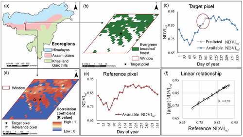
Certain selection conditions are defined in the algorithm to search for nominee pixels to become a reference pixel, i.e. NDVI_ref at a pixel (a, b) with valid values to restore affected NDVI_ref at the target pixel, i.e. NDVI_ref at (i, j). The selection conditions for nominee pixels are listed as follows.

1. LULC of target and nominee pixel must be same.

2. Coefficient of correlation between target and nominee pixels within the window must be more than limit (L ≥ 0.9).

3. Percentage of valid data at nominee pixel must be more than that of target pixel.

4. There must not be null data in both the target and nominee pixel at same temporal position, k.

Out of all nominee pixels listed within the window, pixel having highest R value with the target pixel is finalized as the reference pixel (pixel with most similar conditions). Later, NDVI_ref curves from reference and target pixels are used in Eq. 6 to draw out coefficients of their linear regression and utilized to restore NDVI_ref curve in target pixel as shown in Eq. 7.

(6) ${\mathrm{N}\mathrm{D}\mathrm{V}\mathrm{I}}_{ref}^{i,j}=m{\mathrm{N}\mathrm{D}\mathrm{V}\mathrm{I}}_{ref}^{a,b}+c$(6)

(7) ${\mathrm{N}\mathrm{D}\mathrm{V}\mathrm{I}}_{ref,k}^{i,j}=m{\mathrm{N}\mathrm{D}\mathrm{V}\mathrm{I}}_{ref,k}^{a,b}+c$(7)

where (i,j) is spatial location of target pixel, (a,b) is the spatial location of reference pixel within the window, m and c are the slope and the intercept for the linear regression between target and reference pixel, and k is the temporal position of target pixel affected with null data. Since, linear regression is used to restore NDVI_ref at target pixel, the restored value might exceed the maximum value of 1 due to which reference pixel is selected which yields a value between 0 and 1. Also, an additional constraint as threshold (T ≥ 50%) is considered below which NDVI_ref having percentage of valid values is rejected as target and skipped due to weak statistics. A typical demonstration of restoration of NDVI_ref is presented in Figure 5.

Restoration of affected NDVI_ref curves throughout the study area was achieved in two stages depending upon static and dynamic LULC in 16 years (2001–2016). In SFA, the window with target pixel at its center is moved in a recursive manner throughout the study area. Its recursion starts by restoring affected NDVI_ref at pixels over 95% valid data and stepping down to 5% with each recursion till pixels with NDVI_ref over 50% valid data is reached as shown in the flowchart in Figure 4. Restoration of affected NDVI_ref for the pixels with static LULC was achieved in the first stage. It was followed by second stage where pixels with dynamic LULC were targeted. In the second stage, pixels with more than four LULC in 16 years were not considered as target pixels due to insufficient NDVI observations to begin with. During the process of restoration, newly produced synthetic values in restored NDVI_ref at any pixel were made accessible for being a nominee in the restoration of other affected pixels. The recursive search and fill process ensures equitable availability of valid values in NDVI_ref. However, definition of W, T and L is dependent upon availability of NDVI data, and hence it is customized as user-defined variables.

2.3.4. Moving offset method (MOM)

NDVI is a proxy for natural vegetation greenness and its temporal variation should be smooth and continuous (Julien and Sobrino 2010). Moreover, this variation is supposed to be nonlinear with time (Verma and Dutta 2013). Therefore, it was assumed that the temporal continuity of NDVI changes from one point of time to another continuously and nonlinearly, but tends to follow the local phenology. The offset of valid NDVI points to its corresponding points on SNDVI_ref at the extreme of missing span are linearly interpolated. Later, missing NDVI values are predicted by adding the interpolated results with the points at SNDVI_ref. By the virtue of moving the linearly interpolated offsets on reference phenology curve, this method of prefilling is named as moving offset method (MOM). This method was directly used for prefilling NDVI time series with the help of SNDVI_ref time series of same time length (viz. 16 years of study period). For a pixel with static LULC, the annual SNDVI_ref curve was repeated 16 times to make SNDVI_ref time series. However, for a pixel with dynamic LULC, we obtained more than one SNDVI_ref curve (Section 2.3.2). Each of these curves represents the reference phenology for different LULC that have existed in 16 years in at the pixel. Therefore, these curves were arranged in order of existent LULC in respective years to produce the SNDVI_ref time series.

A conceptual demonstration of MOM for prefilling the missing NDVI is presented in Figure 6. In the figure, NDVI at time slots 2, 3, and 4 are missing which needs to be filled. W₁ and W₅ represent the offset of NDVI from SNDVI_ref time series at the extreme ends of missing span. The offsets between W₁ and W₅ were linearly interpolated and adding the results to the SNDVI_ref curve predicted missing NDVI at positons 2, 3 and 4, which also tends to follow the local phenology. Missing span at the extreme ends of time series is linearly extrapolated in similar manner. The completed NDVI series were considered to be as good as MVC composites which are further subjected to application of HANTS.

Figure 6. Conceptual demonstration of moving offset method for prefilling of NDVI time series.

2.4. Evaluation strategy for performance of MOM with HANTS

MOM was compared with other popular interpolation methods (IDW and cubic spline) for checking its robustness in prefilling the NDVI time series. Years with highest NDVI data availability in the time series at one virtual station from each ecoregions having major LULC percentage (as shown in Section 2.2.3) were selected. Afterwards, annual NDVI data were intentionally reduced from the mid year. The reduced annual data was applied to the three prefilling methods MOM, IDW and cubic spline. The variation of R² value with decrease in valid data reflects the robustness of predictions by the prefilling methods.

A comparative analysis between reconstructed NDVI time series by four approaches at the virtual stations and in the study area was also conducted. The approaches are (i) HANTS (HA), (ii) IDW prior to HANTS (IHA), (iii) cubic spline prior to HANTS (SHA), and (iv) MOM prior to HANTS (MHA). The parameter settings for application of HANTS to reconstruct annual time series are shown in Table 2. We also included comparison of seasonality trait and fitting performance for overall evaluation of efficiency of reconstruction methods.

The seasonality trait was evaluated on the basis of visual interpretation of anomalies in high, low, and transition seasonal values in reconstructed NDVI within the span of years 2001–2016 at virtual stations. The fitting performance of reconstructed NDVI was evaluated on the basis of three indicators. The first indicator is linearity of reconstructed NDVI time series (RNDVI) with SNDVI_ref time series represented by correlation coefficient (R value). This value represents the capability of approach to reconstruct NDVI time series following local phenology, which is reasonable according to seasonality trait. The second indicator is a quantity called as normalized noise-related error (NNRE) which is proposed by Zhou et al. (2016) as fitting evaluation standards. NNRE is the normalized difference of fitting method related error (FRE) and overall reconstruction error (ORE) as described in Eq. 8 to 10.

(8) $\mathrm{F}\mathrm{R}\mathrm{E}=\sqrt{\frac{\sum _{i=1}^n{\left(\mathrm{S}\mathrm{N}\mathrm{D}\mathrm{V}{\mathrm{I}}_{ref}-\mathrm{N}\mathrm{D}\mathrm{V}{\mathrm{I}}_{ref}\right)}^2}{n}}$(8)

(9) $\mathrm{O}\mathrm{R}\mathrm{E}=\sqrt{\frac{\sum _{i=1}^n{\left(\mathrm{R}\mathrm{N}\mathrm{D}\mathrm{V}\mathrm{I}-\mathrm{N}\mathrm{D}\mathrm{V}{\mathrm{I}}_{ref}\right)}^2}{n}}$(9)

(10) $\mathrm{N}\mathrm{N}\mathrm{R}\mathrm{E}=\left(\mathrm{O}\mathrm{R}\mathrm{E}-\mathrm{F}\mathrm{R}\mathrm{E}\right)/\left(\mathrm{O}\mathrm{R}\mathrm{E}+\mathrm{F}\mathrm{R}\mathrm{E}\right)$(10)

where SNDVI_ref is fitted reference phenology curve, NDVI_ref is the reference phenology curve, and RNDVI is reconstructed NDVI time series, n is respective number of elements.

The ORE expresses the overall reconstruction performance, while FRE estimates the accuracy of the mathematical descriptors of the reconstruction models. The NNRE can effectively represent good fit by utilization of available data. On a scale of −1 to 1, larger NNRE means a weaker influence of FRE on overall reconstruction or bad fit whereas small NNRE means the ORE can be mainly explained by FRE or good fit. A common way of evaluation of the overall reconstruction performance is on the basis of the total difference between reconstructed and reference series as formulated in ORE (Zhou et al. 2016; Zhou, Jia, and Menenti 2015; Geng, Ma, and Wang 2016). Being a version of root mean square error, it is considered that lower ORE values represent relatively better fit. The ORE has the potential to show overall severity of error magnitudes in reconstruction. However, NNRE could be helpful in magnifying the results in order to evaluate.

3. Results

3.1. Selection of window size

There could be number of pixels with similar phenology trait having same LULC in the study area out of which only one pixel with best similarity with the target pixel is selected as the reference pixel by the SFA within a moving window. The size of window (W) is an important factor to secure the study area with maximum number of complete NDVI_ref and proceed for successful implementation of MOM. Selecting too large W might delay the searching process whereas too small W might fail to capture nominee pixels to become the reference pixel. Therefore, selection of a suitable W for SFA was a keen necessity.

Figure 7 supports the decision-making process for selection of a suitable W by illustration at the virtual stations. Considering the virtual stations as pseudo target pixels, we calculated R value between virtual stations and its respective nominees for reference pixel in the same ecoregion (applied with conditions as discussed in Section 2.3.3). Also, the spatial distance (Euclidean distance) between the virtual station and its respective nominee pixels were calculated for deciding W. The subplots in Figure 7 show the scatterplot between these R values against corresponding spatial distance. Since, the aim of the window is to find most similar nominee pixel, 99th percentile for R values was used to separate most probable nominee pixels which are most likely to get selected for the reference pixel. The line connecting nominees over 99th percentile in the scatter map is referred as 99th percentile isoline. The main graph of Figure 7 displays the 99th percentile isoline with its linear trend. Most of the virtual stations show a declining trend with increase in distance, while two of them show near-stability. It suggests that increasing W is probable to reduce the chances of getting better nominees for reference pixel with obvious delay in processing time. A common W for moving window was to be set for entire study areas due to which the decision had to be on broad considerations as trade-off between processing time and similarity of nominee pixels. The vertical dashed lines are the 25 km threshold within which suitable number of nominee pixels could be found. Thus, for restoration of incomplete NDVI_ref with most linear NDVI_ref satisfying selection conditions within a window size of (W ≈ 25 km²) was decided in this work. However, the size of W might differ for different data series as well as regions.

Figure 7. Scatter plot between correlation coefficient (R value) against spatial distance at various virtual stations where, R value is correlation coefficient between NDVI_ref curves at virtual station and its nominee pixels, and spatial distance is distance between virtual station and its nominee pixels. The plot is shown for virtual stations (a) VS1, (b) VS2, (c) VS3, (d) VS4, (e) VS5, (f) VS6, (g) VS7, (h) VS8, and (i) VS9.

3.2. Performance of MOM

3.2.1. Robustness of MOM

The virtual stations, VS1 (mixed forest), VS4 (agriculture), and VS7 (evergreen broadleaf forest) were selected for checking the robustness of MOM. For VS1 and VS4, year 2006 was found as the least problematic year with a data availability of 86.9% and 73.9%, respectively. Similarly, year 2001 was found least problematic with a data availability of 95.7% for VS7. Figure 8 shows the coefficient of determination (R² value) for interpolating the missing NDVI values in the year with variable data gaps against original NDVI values. We checked the performance of the three methods (MOM, IDW, and cubic spline) at VS1 with data availability of 86.9%, 69.6%, and 47.5% (Figure. 8(a–c)); VS1 with data availability of 73.9%, 60.9%, and 47.5% (Figure. 8(d–f)); and VS1 with data availability of 86.9%, 69.6%, and 47.5% (Figure. 8(g–i)). Since, the first set of graphs (Figure. 8(a, d, and g)) are plots for interpolated NDVI against original NDVI in the respective years, it shows R² value as 1 for all the methods. However, an overall decline in R² value for all the methods at all virtual stations could be seen with decrease in data percentage. MOM is found with better predictions than IDW and cubic spline in VS1 and VS4 with R² value over 0.8 (Figure 8(b, c, e, f)), while at VS7, cubic spline was found as the best predicting method with R² value over 0.8 where MOM was moderate with R² value of 0.78 (Figure 8(i)). However, both cubic spline and IDW methods failed during low data availability at VS1 (Figure 8(c)) and VS4 (Figure 8(f)), respectively (with R² value under 0.5 in both cases). Therefore, it can be considered that MOM is more robust for predicting NDVI time series in variable data gap conditions than IDW and cubic spline methods.

Figure 8. Performance of MOM, IDW, and cubic spline interpolation methods in prefilling NDVI time series at virtual stations. Prefilling at VS1 in year 2006 with data availability of (a) 86.9% (original data), (b) 69.6%, and (c) 47.5%. Prefilling at VS3 in year 2006 with data availability of (d) 73.9%, (e) 60.9%, and (f) 34.8%. Prefilling at VS7 in year 2001 with data availability of (g) 95.7%, (h) 73.9%, and (i) 47.9%.

3.2.2. Seasonality trait in different approaches

The seasonality trait is based on visual interpretation of surface plot of time series against years where the anomalies in seasonal high, low and transition is compared during reconstruction span. The reconstructed time series for VS1, VS4 and VS7 are shown in Figure 9. The color scheme provided in the figure is concise between low and high value for scaling as indicated in the legends; however lowest magnitude might represent underestimations. The most problematic years on the basis of data availability were years 2015 and 2016 for VS1, years 2008, 2012 and 2016 for VS4 and year 2016 for VS7 which could be clearly identified in plot for raw NDVI. Due to long gaps of missing values in above-mentioned years, direct application of HA with the parameter settings (Table 2) is not able to reconstruct values in respective seasonal range. Rather, HA predicted a series of low values (as set in low threshold setting in Table 2) in this time. It shows failure of direct application of HA to long data gaps.

Figure 9. The sixteen annual NDVI series for the virtual stations by different approaches (HA, MHA, IHA, and SHA). (a) VS1: Mixed forest, (b) VS4: Agriculture, (c) VS7: Evergreen broadleaf forest. (Note: interpretations in the marked areas are discussed in Section 3.2.2).

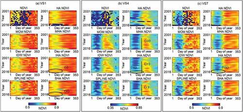
Addition of an interpolation method prior to application of HANTS was helpful in overcoming this problem. However, visual interpretation of Figure 9 shows the shortcomings of IHA and SHA as compared to MHA. For VS1 (mixed forest), the mark near (i) shows that IHA was unable to identify seasonal low and overestimates in years 2015 and 2016. A similar overestimation was seen by SHA in year 2016 as shown in mark near (ii). But MHA was observed to predict seasonal low properly in the years 2015 and 2016 for VS1. For VS4 as agriculture, the occurrence of dormant and peak seasons are equally important where a clear boundary separating the two seasons is logical due to yearly crop calendar and human activities. A visual comparison between vertical lines drawn near (iii), (iv), and (v) shows that division between dormant and agricultural season is more prominent for the case of MHA than IHA and SHA. Also, IHA was unable to reconstruct seasonal low in year 2016 as shown at mark near (vi), whereas MHA and SHA succeeded. For VS7 (evergreen broadleaf forest), all MHA, IHA, and SHA performed similarly except for that IHA failed to reconstruct seasonal low in 2016 as shown at mark near (vii). From visual observation, it was found that MHA satisfied most of the details of seasonality trait for virtual stations as compared to HA, IHA, and SHA.

3.2.3. Fitting performance

Fitting indicators along with linearity with reference phenology curve were compared to evaluate fitting performance. In our study, ORE for different methods is normalized with same FRE to get different NNRE for different approaches at a single virtual station. Therefore, ORE and NNRE signify best-performing method in same sense. Indicators of fitting performance i.e. R, ORE, FRE, and NNRE for 16-daily time series at virtual stations of the study area are presented in Table 3.

Table 3. Indicators of fitting performance at virtual stations in the study area (Note: Best values are represented in bold).

Virtual Station	R				ORE				FRE	NNRE
	HA	IHA	SHA	MHA	HA	IHA	SHA	MHA		HA	IHA	SHA	MHA
VS1	0.4507	0.7643	0.6567	0.8026	0.1291	0.0644	0.0649	0.0636	0.0084	0.8778	0.7692	0.7708	0.7666
VS2	0.2750	0.8613	0.8190	0.8690	0.0991	0.0311	0.0367	0.0321	0.0084	0.8437	0.5746	0.6274	0.5851
VS3	0.3568	0.9379	0.8772	0.9655	0.1888	0.0609	0.0728	0.0419	0.0204	0.8049	0.4981	0.5622	0.3451
VS4	0.6156	0.8903	0.8952	0.9334	0.1238	0.0567	0.0548	0.0483	0.0273	0.6386	0.3500	0.3349	0.2777
VS5	0.9264	0.9617	0.9396	0.9694	0.0575	0.0429	0.0473	0.0411	0.0147	0.5927	0.4895	0.5258	0.4731
VS6	0.7588	0.9008	0.9101	0.9303	0.0875	0.0461	0.0469	0.0426	0.0344	0.4356	0.1453	0.1537	0.1064
VS7	0.6942	0.9229	0.9234	0.9375	0.0852	0.0392	0.0403	0.0373	0.0099	0.7917	0.5967	0.6055	0.5805
VS8	0.6729	0.9524	0.9186	0.9634	0.0970	0.0366	0.0408	0.0333	0.0147	0.7367	0.4269	0.4702	0.3875
VS9	0.9726	0.9730	0.9734	0.9746	0.0386	0.0443	0.0402	0.0390	0.0204	0.3084	0.3693	0.3267	0.3131

It shows that ORE exceeded the error limit of 0.05 with highest values at most of the instances for HA. The worst performance is mainly due to inability of HA to reconstruct at large data gaps. Addition of an interpolation prior to application of HANTS reduced this error remarkably. However, except for VS1, methods other than MHA could not reduce ORA below 0.05. The FRE always stayed below 0.05. It is only at VS9 that HA performed best due to least problems in large data gaps in original time series. MHA performed best with lowest ORE and NNRE at majority of virtual stations (VS1, VS3, VS4, VS5, VS6, VS7, and VS8). In other cases, IHA performed best at VS2, but the performance of MHA at VS2 was second best with marginal difference in NNRE than that of IHA. MHA was also seen having NNRE with slim difference to that of HA at VS9. It was seen that unlike HA, IHA, and SHA, on the basis of ORE and NNRE, the performance of MHA is either best or second best with marginal difference than that of the best method. Also, the correlation coefficient (R value) of MHA with local reference phenology curve is highest for all the virtual stations. It signifies that MHA have more capability to restore local phenology pattern in reconstructed NDVI time series which is reasonable according to seasonality trait. On an overall understanding, MHA was able to effectively fit the shortcomings which were faced with HA.

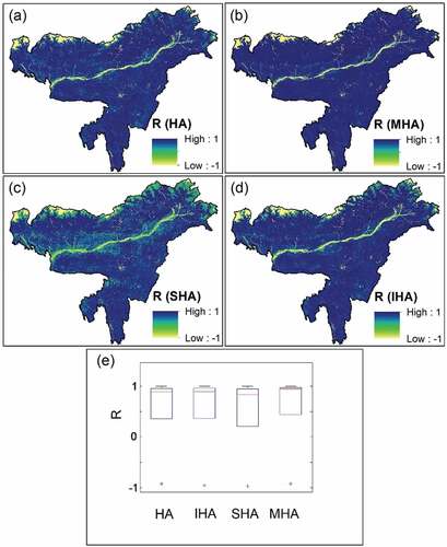
Figure 10 shows the overall fitting performance of HA, MHA, IHA, and SHA approaches over the study area. The distribution of NNRE in the boxplots shows that overall population between the 1st and 3rd quartiles along with median is least in case of MHA from all other approaches. The spatial averages of NNRE for the study area with various approaches were found as 0.21, 0.25, 0.29, and 0.19 for HA, IHA, SHA, and MHA, respectively. It indicates that a major part of the study area have reduced NNRE, which means better fitting performance by MHA than other approaches. Similar comparison for coefficient of correlation with reference land surface phenology in Figure 11 shows maximum R for MHA. The spatial averages of R for the study area with various approaches were found as 0.78, 0.77, 0.64, 0.88 for HA, IHA, SHA, and MHA, respectively. It means reconstructed NDVI time series from MHA has better association with seasonality trait.

Figure 10. Fitting performance in the study area by HANTS without and with prefilling methods. (a) NNRE by HA approach. (b) NNRE by IHA approach. (c) NNRE by SHA approach. (d) NNRE by MHA approach. (e) Distribution of NNRE by different approaches.

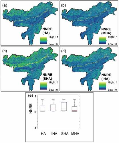
Figure 11. Seasonal performance shown as R with corresponding reference phenology curve in the study area by HANTS without and with prefilling methods. (a) R by HA approach. (b) R by IHA approach. (c) R by SHA approach. (d) R by MHA approach. (e) Distribution of R by different approaches.

4. Discussion

4.1. Practical problems in direct application of HANTS

Consistent availability of high-quality spatiotemporal NDVI time series data (e.g. MODIS/SPOT/AVHRR, etc.) is important for various terrestrial studies. It has led to development of several reconstruction methods in past two decades and their use has grown with wide research interests. However, most of these methods draw information from the available NDVI time series data at a particular pixel to reconstruct itself. Most of the times, this approach of temporal dependence is limited when the time series is met by large data gaps. HANTS is one among those methods with similar limitations. NDVI time series with large data gaps due to seasonal obstructions, technical glitches in sensors, or anonymous reasons, return a series of low values on application of HANTS.

This could be seen for HA NDVI at virtual stations, VS1, VS4, and VS7 (Figure. 9(a–c)). The problem is insufficient observation frequency in the times-series due to which large gap with null data is available within the range of degree of overdeterminedness (Section 2.3.1). Hence, a lot of observations with low values influence the fitting curve to move toward the low values with increase in iterations inside HANTS algorithm till the final curve finds itself within the distance of fit error tolerance (Section 2.3.1). This problem could be either solved by changing the parameter settings or increasing the observation frequency with reasonable values. The re-adjustment of parameter settings can always improve the curve fitting. However, it can degrade the physical significance of variation in NDVI which makes the latter approach more reliable.

4.2. Difference between MOM and other interpolation methods

Recently, new approaches have emerged which includes prefilling of NDVI time series prior to application of reconstruction methods. In this work, we hypothesized that vegetation in the missing span should vary according to a general pattern of reference phenology at the pixel (Section 2.3.4). In case of absence of valid data in reference phenology, it was supported by a unique recursive SFA applied in two stages for pixels with static and dynamic LULC, respectively (Section 2.3.3). The SFA restores null data in reference phenology curve of a target pixel by regression model (Eq. 6 and 7) using specific relationship with the reference phenology curve of a reference pixel within a defined spatial extent (most similar conditions defined in Section 2.3.3). In this way, spatiotemporal information is directly reflected in prefilling by MOM in data deficient cases. The expected advantage of MOM interpolation was found over IDW and cubic spline methods (Figure 8). Addressing robustness while predicting NDVI time series is uncertain given interpolation methods such as IDW and cubic spline are based on mathematical formulations; especially during large data gaps. In contrast, including the reference phenology for controlling the trajectory of interpolation makes MOM a robust interpolation technique for NDVI time series.

It also reflects the failure of IDW and cubic spline to follow the seasonality trait in Figure 9 (IDW NDVI and HANTS NDVI). Since, application of HANTS presumes the prefilled data as observations; their respective returned fitted curves are also forced to behave the same way (IHA and SHA in Figure 9). As a result, the seasonality trait is lost which reduces the quality of reconstructed NDVI time series. Contrastingly, MHA is not seen to face these deformations due to robust prefilling performance by MOM.

4.3. Scope and limitations of MOM with HANTS

The approach used to prefill the NDVI time series by MOM prior to application of HANTS, helps in increasing observation frequency with values in reliable range in data deficient pixels. Predictions made by MOM are mainly dependent on the local reference phenology at each pixel. Therefore, this approach is expected to work for regions having long-term applications of NDVI time series data. It might be noted that annual LULC time series data is the only additional data which was used in this study. There are various sources of NDVI time series data with annual LULC counterparts (e.g. MODIS/AVHRR/SPOT/Landsat, etc.), which extends the scope of this work in long-term global applications (e.g. deforestation monitoring, agricultural drought, etc.) Since, this study evaluated the performance of HANTS with and without prefilling with MOM in one of the frequently clouded regions as the study area (Figures 10 and 11), the proposed prefilling method can be considered suitable for other regions of the world with good confidence.

However, there are some aspects which restrict the proposed approach in specific conditions. First, the chances of preparation of a reference phenology curve reduce at a pixel with frequently changing LULC with time. Hence, this method is unsuitable for regions with frequent changes in LULC within a short span of time. It is because of possible contrast in reference phenology in the pixel and real-time NDVI variations. This restricts the use of the proposed approach in short-term applications (e.g. flood inundation). To filter such pixels, the variability of LULC till a maximum of four classes was constrained in this study. Second, the used LULC data should be accurate to support the approach. Inaccurate LULC data can deform the restoration of reference phenology by recursive SFA which can further reduce the robustness of MOM. Third, recursive SFA in this approach restores the reference phenology at a pixel depending upon spatial similarity of phenology within a limited window region (W). So, the heterogeneous regions reliant on anthropogenic sources, e.g. agricultural areas, are likely to be affected. Nevertheless, as long as regional homogeneity within the window exists, there is no major issue. And lastly, increasing the spatiotemporal consistency in NDVI can support emerging studies such as spatial downscaling and image fusion (Bindhu and Narasimhan 2015; Boyte et al. 2018). But, with limitation of MOM confined to be used for reconstruction of NDVI time series in vegetated areas, it might fail to address issues such as urban expansion (Pandey, Zhang, and Seto 2018). Therefore, it might not be useful for non-vegetated terrestrial classes (e.g. snow, water bodies, sand, urban areas, etc.)

5. Conclusion

This study gives a spatiotemporal comparison of the reconstruction performance by using HANTS on original and prefilled NDVI time series data. The comparison is based on the MODIS 16-day composite NDVI time series dataset having 23 samples in an annual series. It was found that prefilling by an interpolation method prior to application of HANTS is helpful in overcoming problems faced by direct application of HANTS during long data gaps. The proposed prefilling method, i.e. moving offset method (MOM) was found to be more robust in comparison to general interpolation methods (IDW and cubic spline) in variable data gap conditions. Spatiotemporal comparison of seasonal as well as fitting performance evaluated for years 2001–2016 revealed that the proposed approach to apply MOM prior to HANTS (MHA) can perform better than similar approaches with general interpolation methods. The NNRE for MHA was found to be lowest than other approaches (spatial average of 0.19). Also, in maintaining the seasonal trait, correlation with general phenology R was found to be highest than other approaches (spatial average of 0.88). It is concluded that MHA produces least fitting errors with highest similarity to existing land surface phenology, thereby justifying the seasonality trait. One major advantage of this scheme is overcoming long gaps by using information from spatial similarity in phenology which is helpful in data deficient scenario. MOM is concluded as a prerequisite of HANTS in spatiotemporal reconstruction which effectively restores the cyclic pattern of land surface vegetation in land-use/land-cover classes. This study could be helpful in enhancing quality of NDVI reconstruction by HANTS for regional scales around the globe.

Highlights

• A novel prefilling method based on regional land surface phenology is proposed

• Evaluation of three prefilling methods to enhance performance of HANTS

• Results from HANTS is improved in variable data gap conditions

Acknowledgments

Authors’ sincere appreciation is extended to NASA and USGS for providing free access to various MODIS products used in this work. Authors also acknowledge the editor and anonymous reviewers.

Disclosure statement

No potential conflict of interest was reported by the authors.

References

- Ahmed, M., B. Else, L. Eklundh, J. Ardö, and J. Seaquist. 2017. “Dynamic Response of NDVI to Soil Moisture Variations during Different Hydrological Regimes in the Sahel Region.” International Journal of Remote Sensing 38: 5408–5429. doi:10.1080/01431161.2017.1339920.
- Anav, A., Q. Liu, A. De Marco, C. Proietti, F. Savi, E. Paoletti, and S. Piao. 2018. “The Role of Plant Phenology in Stomatal Ozone Flux Modeling.” Global Change Biology 24: 235–248. doi:10.1111/gcb.13823.
- Atzberger, C., and P. H. C. Eilers. 2011a. “A Time-series for Monitoring Vegetation Activity and Phenology at 10-daily Time Steps Covering Large Parts of South America.” International Journal of Digital Earth 4 (5): 365–386. doi:10.1080/17538947.2010.505664.
- Atzberger, C., and P. H. C. Eilers. 2011b. “Evaluating the Effectiveness of Smoothing Algorithms in the Absence of Ground Reference Measurements.” International Journal of Remote Sensing 32: 3689–3709. doi:10.1080/01431161003762405.
- Azzali, S., and M. Menenti. 2000. “Mapping Vegetation-soil-climate Complexes in Southern Africa Using Temporal Fourier Analysis of NOAA-AVHRR NDVI Data.” International Journal of Remote Sensing 21 (5): 973–996. doi:10.1080/014311600210380.
- Beck, P. S. A., C. Atzberger, K. A. Høgda, B. Johansen, and A. K. Skidmore. 2006. “Improved Monitoring of Vegetation Dynamics at Very High Latitudes: A New Method Using MODIS NDVI.” Remote Sensing of Environment 100 (3): 321–334. doi:10.1016/J.RSE.2005.10.021.
- Bindhu, V. M., and B. Narasimhan. 2015. “Development of a Spatio-Temporal Disaggregation Method (disndvi) for Generating a Time Series of Fine Resolution NDVI Images.” ISPRS Journal of Photogrammetry and Remote Sensing 101: 57–68. doi:10.1016/J.ISPRSJPRS.2014.12.005.
- Boyte, S. P., B. K. Wylie, M. B. Rigge, and D. Dahal. 2018. “Fusing MODIS with Landsat 8 Data to Downscale Weekly Normalized Difference Vegetation Index Estimates for Central Great Basin Rangelands, USA.” GIScience & Remote Sensing 55 (3): 376–399. doi:10.1080/15481603.2017.1382065.
- Bucha, T., and M. Koren. 2017. “Phenology of the Beech Forests in the Western Carpathians from MODIS for 2000-2015.” iForest 10 (3): 537. doi:10.3832/IFOR2062-010.
- Carreiras, J. M. B., J. M. C. Pereira, Y. E. Shimabukuro, and D. Stroppiana. 2003. “Evaluation of Compositing Algorithms over the Brazilian Amazon Using SPOT-4 VEGETATION Data.” International Journal of Remote Sensing 24 (17): 3427–3440. doi:10.1080/0143116021000021251.
- Carter, E., C. Hain, M. Anderson, and S. Steinschneider. 2018. “A Water Balance–Based, Spatiotemporal Evaluation of Terrestrial Evapotranspiration Products across the Contiguous United States.” Journal of Hydrometeorology 19: 891–905. doi:10.1175/JHM-D-17-0186.1.
- Chen, J., P. Jönsson, M. Tamura, Z. Gu, B. Matsushita, and L. Eklundh. 2004. “A Simple Method for Reconstructing A High-quality NDVI Time-series Data Set Based on the Savitzky–Golay Filter.” Remote Sensing of Environment 91 (3–4): 332–344. doi:10.1016/J.RSE.2004.03.014.
- Chen, X. 2017. Spatiotemporal Coupling Effects of Plant Phenology. 91–96. Berlin, Heidelberg, Germany:Springer. doi:10.1007/978-3-662-49839-2_9.
- de Beurs, K. M., and G. M. Henebry. 2005. “A Statistical Framework for the Analysis of Long Image Time-series.” International Journal of Remote Sensing 26 (8): 1551–1573. doi:10.1080/01431160512331326657.
- Didan, K. 2015. “MOD13A1 MODIS/Terra Vegetation Indices 16-day L3 Global 500m SIN Grid V006 [data Set].” NASA EOSDIS LP DAAC. doi: 10.5067/MODIS/MOD13A1.006.
- Fischer, A. 1994. “A Model for the Seasonal Variations of Vegetation Indices in Coarse Resolution Data and Its Inversion to Extract Crop Parameters.” Remote Sensing of Environment 48 (2): 220–230. doi:10.1016/0034-4257(94)90143-0.
- Friedl, M., D. McIver, J. C. Hodges, X. Zhang, D. Muchoney, A. Strahler, C. Woodcock, et al. 2002. “Global Land Cover Mapping from MODIS: Algorithms and Early Results.” Remote Sensing of Environment 83 (1–2): 287–302. doi:10.1016/S0034-4257(02)00078-0.
- Gandhi, G. M., S. Parthiban, N. Thummalu, and A. Christy. 2015. “Ndvi: Vegetation Change Detection Using Remote Sensing and GIS – A Case Study of Vellore District.” Procedia Computer Science 57: 1199–1210. doi:10.1016/J.PROCS.2015.07.415.
- Garonna, I., R. de Jong, R. Stöckli, B. Schmid, D. Schenkel, D. Schimel, and M. E. Schaepman. 2018. “Shifting Relative Importance of Climatic Constraints on Land Surface Phenology.” Environmental Research Letters 13 (2): 024025. doi:10.1088/1748-9326/aaa17b.
- Geerken, R., B. Zaitchik, and J. P. Evans. 2005. “Classifying Rangeland Vegetation Type and Coverage from NDVI Time-series Using Fourier Filtered Cycle Similarity.” International Journal of Remote Sensing 26 (24): 5535–5554. doi:10.1080/01431160500300297.
- Geng, L., M. Ma, and H. Wang. 2016. “An Effective Compound Algorithm for Reconstructing MODIS NDVI Time-series Data and Its Validation Based on Ground Measurements.” IEEE Journal of Selected Topics in Applied Earth Observations and Remote Sensing 9 (8): 3588–3597. doi:10.1109/JSTARS.2015.2495112.
- Geng, L., M. Ma, X. Wang, W. Yu, S. Jia, and H. Wang. 2014. “Comparison of Eight Techniques for Reconstructing Multi-satellite Sensor Time-series NDVI Data Sets in the Heihe River Basin, China.” Remote Sensing 6 (3): 2024–2049. doi:10.3390/rs6032024.
- Glennie, E., and A. Anyamba. 2018. “Midwest Agriculture and ENSO: A Comparison of AVHRR NDVI3g Data and Crop Yields in the United States Corn Belt from 1982 to 2014.” International Journal of Applied Earth Observation and Geoinformation 68: 180–188. doi:10.1016/J.JAG.2017.12.011.
- Gokmen, M., Z. Vekerdy, W. Verhoef, and O. Batelaan. 2013. “Satellite-based Analysis of Recent Trends in the Ecohydrology of a Semi-arid Region.” Hydrology and Earth System Sciences 17: 3779–3794. doi:10.5194/hess-17-3779-2013.
- Gu, J., X. Li, C. Huang, and G. S. Okin. 2009. “A Simplified Data Assimilation Method for Reconstructing Time-series MODIS NDVI Data.” Advances in Space Research 44 (4): 501–509. doi:10.1016/J.ASR.2009.05.009.
- Holben, B. N. 1986. “Characteristics of Maximum-value Composite Images from Temporal AVHRR Data.” International Journal of Remote Sensing 7 (11): 1417–1434. doi:10.1080/01431168608948945.
- Huete, A., C. Justice, and W. Van Leeuwen. 1999. “MODIS Vegetation Index (MOD 13) Algorithm Theoretical Basis Document Version 3.” https://modis.gsfc.nasa.gov/data/atbd/atbd_mod13.pdf
- Huete, A., K. Didan, T. Miura, E. Rodriguez, X. Gao, and L. Ferreira. 2002. “Overview of the Radiometric and Biophysical Performance of the MODIS Vegetation Indices.” Remote Sensing of Environment 83 (1–2): 195–213. doi:10.1016/S0034-4257(02)00096-2.
- Jain, S. K., V. Kumar, and M. Saharia. 2013. “Analysis of Rainfall and Temperature Trends in Northeast India.” International Journal of Climatology 33 (4): 968–978. doi:10.1002/joc.3483.
- Jaswal, A. K., P. A. Kore, and V. Singh. 2017. “Variability and Trends in Low Cloud Cover over India during 1961-2010.” Mausam 68 (2): 235–252.
- Jia, L., H. Shang, G. Hu, and M. Menenti. 2011. “Phenological Response of Vegetation to Upstream River Flow in the Heihe River Basin by Time-series Analysis of MODIS Data.” Hydrology and Earth System Sciences 15 (3): 1047–1064. doi:10.5194/hess-15-1047-2011.
- Jiang, D., H. Zhang, Y. Zhang, and K. Wang. 2014. “Interannual Variability and Correlation of Vegetation Cover and Precipitation in Eastern China.” Theoretical and Applied Climatology 118: 93–105. doi:10.1007/s00704-013-1054-2.
- Joiner, J., Y. Yoshida, M. Anderson, T. Holmes, C. Hain, R. Reichle, R. Koster, E. Middleton, and F.-W. Zeng. 2018. “Global Relationships among Traditional Reflectance Vegetation Indices (NDVI and NDII), Evapotranspiration (ET), and Soil Moisture Variability on Weekly Timescales.” Remote Sensing of Environment 219: 339–352. doi:10.1016/J.RSE.2018.10.020.
- Jönsson, P., and L. Eklundh. 2004. “TIMESAT—A Program for Analyzing Time-series of Satellite Sensor Data.” Computers & Geosciences 30 (8): 833–845. doi:10.1016/J.CAGEO.2004.05.006.
- Julien, Y., and J. A. Sobrino. 2010. “Comparison of Cloud-reconstruction Methods for Time-series of Composite NDVI Data.” Remote Sensing of Environment 114 (3): 618–625. doi:10.1016/J.RSE.2009.11.001.
- Julien, Y., and J. A. Sobrino. 2019. “Optimizing and Comparing Gap-filling Techniques Using Simulated NDVI Time Series from Remotely Sensed Global Data.” International Journal of Applied Earth Observation and Geoinformation 76: 93–111. doi:10.1016/J.JAG.2018.11.008.
- Jun, W., S. Zhongbo, and M. Yaoming. 2009. “Reconstruction of a Cloud-free Vegetation Index Time Series for the Tibetan Plateau.” Mountain Research and Development 24 (4): 348–354. doi:10.1659/0276-4741(2004)024[0348:ROACVI]2.0.CO;2.
- Justice, C. O., J. R. G. Townshend, B. N. Holben, and C. J. Tucker. 1985. “Analysis of the Phenology of Global Vegetation Using Meteorological Satellite Data.” International Journal of Remote Sensing 6 (8): 1271–1318. doi:10.1080/01431168508948281.
- Kiapasha, K., A. A. Darvishsefat, Y. Julien, J. A. Sobrino, N. Zargham, P. Attarod, and M. E. Schaepman. 2017. “Trends in Phenological Parameters and Relationship between Land Surface Phenology and Climate Data in the Hyrcanian Forests of Iran.” IEEE Journal of Selected Topics in Applied Earth Observations and Remote Sensing 10 (11): 4961–4970. doi:10.1109/JSTARS.2017.2736938.
- Kobayashi, H., and D. G. Dy. 2005. “Atmospheric Conditions for Monitoring the Long-term Vegetation Dynamics in the Amazon Using Normalized Difference Vegetation Index.” Remote Sensing of Environment 97 (4): 519–525. doi:10.1016/J.RSE.2005.06.007.
- Kundu, A., D. M. Denis, N. R. Patel, and D. Dutta. 2018. “A Geo-spatial Study for Analysing Temporal Responses of NDVI to Rainfall.” Singapore Journal of Tropical Geography 39: 107–116. doi:10.1111/sjtg.12217.
- Li, N., L. Jia, and C. Zheng. 2014. “Evaluation of the Harmonic-analysis Method for Surface Soil Heat Flux Estimation: A Case Study in Heihe River Basin.” Proc. SPIE 9260, Land Surface Remote Sensing II, 926043, SPIE Asia-Pacific Remote Sensing, Beijing, China. doi: 10.1117/12.2069270.
- Li, Z., C. Huang, Z. Zhu, F. Gao, H. Tang, X. Xin, L. Ding, et al. 2018. “Mapping Daily Leaf Area Index at 30 M Resolution over a Meadow Steppe Area by Fusing Landsat, Sentinel-2A and MODIS Data.” International Journal of Remote Sensing 39 (23): 9025–9053. doi:10.1080/01431161.2018.1504342.
- Liang, S. Z., W. D. Ma, X. Y. Sui, H. M. Yao, H. Z. Li, T. Liu, X. H. Hou, and M. Wang. 2017. “Extracting the Spatiotemporal Pattern of Cropping Systems from NDVI Time Series Using A Combination of the Spline and HANTS Algorithms: A Case Study for Shandong Province.” Canadian Journal of Remote Sensing 43: 1–15. doi:10.1080/07038992.2017.1252906.
- Lin, C. Y., H. M. Lo, W. C. Chou, and W. T. Lin. 2004. “Vegetation Recovery Assessment at the Jou-Jou Mountain Landslide Area Caused by the 921 Earthquake in Central Taiwan.” Ecological Modelling 176: 75–81. doi:10.1016/J.ECOLMODEL.2003.12.037.
- Liu, D., F. Tian, M. Lin, and M. Sivapalan. 2015. “A Conceptual Socio-hydrological Model of the Co-evolution of Humans and Water: Case Study of the Tarim River Basin, Western China.” Hydrology and Earth System Sciences 19: 1035–1054. doi:10.5194/hess-19-1035-2015.
- Liu, X., X. Zhu, W. Zhu, Y. Pan, C. Zhang, and D. Zhang. 2014. “Changes in Spring Phenology in the Three-Rivers Headwater Region from 1999 to 2013.” Remote Sensing 6 (9): 9130–9144. doi:10.3390/rs6099130.
- Lovell, J. L., and R. D. Graetz. 2001. “Filtering Pathfinder AHRR Land NDVI Data for Australia.” International Journal of Remote Sensing 22 (13): 2649–2654. doi:10.1080/01431160116874.
- Lu, X. L., R. G. Liu, J. Y. Liu, and S. L. Liang. 2007. “Removal of Noise by Wavelet Method to Generate High Quality Temporal Data of Terrestrial MODIS Products.” Photogrammetric Engineering & Remote Sensing 73 (10): 1129–1139. doi:10.14358/PERS.73.10.1129.
- Ma, M., and F. Veroustraete. 2006. “Reconstructing Pathfinder AVHRR Land NDVI Time-series Data for the Northwest of China.” Advances in Space Research 37 (4): 835–840. doi:10.1016/J.ASR.2005.08.037.
- Menenti, M., S. Azzali, W. Verhoef, and R. van Swol. 1993. “Mapping Agroecological Zones and Time Lag in Vegetation Growth by Means of Fourier Analysis of Time-series of NDVI Images.” Advances in Space Research 13 (5): 233–237. doi:10.1016/0273-1177(93)90550-U.
- Morton, D. C., R. S. DeFries, Y. E. Shimabukuro, L. O. Anderson, E. Arai, F. Del Bon Espirito-Santo, R. Freitas, and J. Morisette. 2006. “Cropland Expansion Changes Deforestation Dynamics in the Southern Brazilian Amazon.” Proceedings of the National Academy of Sciences of the United States of America 103 (39): 14637–14641. doi:10.1073/pnas.0606377103.
- Musial, J. P., M. M. Verstraete, and N. Gobron. 2011. “Technical Note: Comparing the Effectiveness of Recent Algorithms to Fill and Smooth Incomplete and Noisy Time-series.” Atmospheric Chemistry and Physics 11 (15): 7905–7923. doi:10.5194/acp-11-7905-2011.
- Padhee, S. K., B. R. Nikam, S. Dutta, and S. P. Aggarwal. 2017. “Using Satellite-based Soil Moisture to Detect and Monitor Spatiotemporal Traces of Agricultural Drought over Bundelkhand Region of India.” GIScience & Remote Sensing 54 (2): 144–166. doi:10.1080/15481603.2017.1286725.
- Panda, S. S., D. P. Ames, and S. Panigrahi. 2010. “Application of Vegetation Indices for Agricultural Crop Yield Prediction Using Neural Network Techniques.” Remote Sensing 2: 673–696. doi:10.3390/rs2030673.
- Pandey, B., Q. Zhang, and K. C. Seto. 2018. “Time Series Analysis of Satellite Data to Characterize Multiple Land Use Transitions: A Case Study of Urban Growth and Agricultural Land Loss in India.” Journal of Land Use Science 13 (3): 221–237. doi:10.1080/1747423X.2018.1533042.
- Park, J. G., R. Tateishi, and M. Matsuoka. 1999. “A Proposal of the Temporal Window Operation (TWO) Method to Remove High-frequency Noises in AVHRR NDVI Time-series Data.” Journal of the Japan Society of Photogrammetry and Remote Sensing 38 (5): 36–47. doi:10.4287/jsprs.38.5_36.
- Ren, J., Z. Chen, Q. Zhou, and H. Tang. 2008. “Regional Yield Estimation for Winter Wheat with MODIS-NDVI Data in Shandong, China.” International Journal of Applied Earth Observation and Geoinformation 10 (4): 403–413. doi:10.1016/J.JAG.2007.11.003.
- Roerink, G. J., M. Menenti, W. Soepboer, and Z. Su. 2003. “Assessment of Climate Impact on Vegetation Dynamics by Using Remote Sensing.” Physics and Chemistry of the Earth, Parts A/B/C 28: 103–109. doi:10.1016/S1474-7065(03)00011-1.
- Roerink, G. J., M. Menenti, and W. Verhoef. 2000. “Reconstructing Cloudfree NDVI Composites Using Fourier Analysis of Time-series.” International Journal of Remote Sensing 21 (9): 1911–1917. doi:10.1080/014311600209814.
- Savitzky, A., and M. J. E. Golay. 1964. “Smoothing and Differentiation of Data by Simplified Least Squares Procedures.” Analytical Chemistry 36 (8): 1627–1639. doi:10.1021/ac60214a047.
- Szabó, S., L. Elemér, Z. Kovács, Z. Püspöki, Á. Kertész, S. K. Singh, and B. Boglárka. 2018. “NDVI Dynamics as Reflected in Climatic Variables: Spatial and Temporal Trends-a Case Study of Hungary.” GIScience & Remote Sensing. doi:10.1080/15481603.2018.1560686.
- Testa, S., K. Soudani, L. Boschetti, and E. Borgogno Mondino. 2018. “MODIS-derived EVI, NDVI and WDRVI Time-series to Estimate Phenological Metrics in French Deciduous Forests.” International Journal of Applied Earth Observation and Geoinformation 64: 132–144. doi:10.1016/J.JAG.2017.08.006.
- Tucker, C. J. 1979. “Red and Photographic Infrared Linear Combinations for Monitoring Vegetation.” Remote Sensing of Environment 8 (2): 127–150. doi:10.1016/0034-4257(79)90013-0.
- Verbesselt, J., R. Hyndman, A. Zeileis, and D. Culveno. 2010. “Phenological Change Detection while Accounting for Abrupt and Gradual Trends in Satellite Image Time-series.” Remote Sensing of Environment 114 (12): 2970–2980. doi:10.1016/J.RSE.2010.08.003.
- Verhegghen, A., S. Bontemps, and P. Defourny. 2014. “A Global NDVI and EVI Reference Data Set for Land-surface Phenology Using 13 Years of Daily SPOT-VEGETATION Observations.” International Journal of Remote Sensing 35 (7): 2440–2471. doi:10.1080/01431161.2014.883105.
- Verhoef, W., M. Menenti, and S. Azzali. 1996. “AColour Composite of NOAA-AVHRR-NDVI Based on Time Series Analysis (1981–1992).” International Journal of Remote Sensing 17 (2): 231–235. doi:10.1080/01431169608949001.
- Verma, R., and S. Dutta. 2013. “Vegetation Dynamics from Denoised NDVI Using Empirical Mode Decomposition.” Journal of the Indian Society of Remote Sensing 41 (3): 555–566. doi:10.1007/s12524-012-0246-z.
- Viovy, N., O. Arino, and A. S. Belward. 1992. “The Best Index Slope Extraction (BISE): A Method for Reducing Noise in NDVI Time-series.” International Journal of Remote Sensing 13 (8): 1585–1590. doi:10.1080/01431169208904212.
- Wang, J., Y. Zhou, L. Zhu, M. Gao, Y. Li, J. Wang, Y. Zhou, L. Zhu, M. Gao, and Y. Li. 2014. “Cultivated Land Information Extraction and Gradient Analysis for a North-South Transect in Northeast Asia between 2000 and 2010.” Remote Sensing 6 (12): 11708–11730. doi:10.3390/rs61211708.
- Wen, J., and Z. Su. 2004. “An Analytical Algorithm for the Determination of Vegetation Leaf Area Index from TRMM/TMI Data.” International Journal of Remote Sensing 25: 1223–1234. doi:10.1080/01431160310001598962.
- Wen, Q., Z. Zhang, S. Liu, X. Wang, and C. Wang. 2010. “Classification of Grassland Types by MODIS Time-series Images in Tibet, China.” IEEE Journal of Selected Topics in Applied Earth Observations and Remote Sensing 3: 404–409. doi:10.1109/JSTARS.2010.2049001.
- Xiao, X., J. Zhang, H. Yan, W. Wu, and C. Biradar. 2009. “Land Surface Phenology.” In Phenology of Ecosystem Processes, edited by A. Noormets, 247–270. New York: Springer. doi:10.1007/978-1-4419-0026-5_11.
- Xiong, Y., and G. Y. Qiu. 2011. “Estimation of Evapotranspiration Using Remotely Sensed Land Surface Temperature and the Revised Three-Temperature Model.” International Journal of Remote Sensing 32: 5853–5874. doi:10.1080/01431161.2010.507791.
- Xu, L., B. Li, Y. Yuan, X. Gao, T. Zhang, L. Xu, B. Li, Y. Yuan, X. Gao, and T. Zhang. 2015. “A Temporal-spatial Iteration Method to Reconstruct NDVI Time Series Datasets.” Remote Sensing 7: 8906–8924. doi:10.3390/rs70708906.
- Yang, J., S. Pan, S. Dangal, B. Zhang, S. Wang, and H. Tian. 2017. “Continental-scale Quantification of Post-fire Vegetation Greenness Recovery in Temperate and Boreal North America.” Remote Sensing of Environment 199: 277–290. doi:10.1016/J.RSE.2017.07.022.
- Zhou, J., L. Jia, and M. Menenti. 2015. “Reconstruction of Global MODIS NDVI Time-series: Performance of Harmonic ANalysis of Time-series (HANTS).” Remote Sensing of Environment 163: 217–228. doi:10.1016/j.rse.2015.03.018.
- Zhou, J., L. Jia, M. Menenti, and B. Gorte. 2016. “On the Performance of Remote Sensing Time-series Reconstruction Methods – A Spatial Comparison.” Remote Sensing of Environment 187: 367–384. doi:10.1016/j.rse.2016.10.025.
- Zhu, W., Y. Pan, H. He, L. Wang, M. Mou, and J. Liu. 2012. “A Changing-Weight Filter Method for Reconstructing A High-quality NDVI Time-series to Preserve the Integrity of Vegetation Phenology.” IEEE Transactions on Geoscience and Remote Sensing 50 (4): 1085–1094. doi:10.1109/TGRS.2011.2166965.