Understanding seasonal dynamics of invasive water hyacinth (Eichhornia crassipes) in the Greater Letaba river system using Sentinel-2 satellite data

Abstract

Water hyacinth (Eichhornia crassipes) is one of the most aggressive and lethal free-floating aquatic weed that degrades and chokes freshwater ecosystems and threatens aquatic life. Early detection and up-to-date information regarding its distribution is, therefore, crucial in understanding its spatial configuration and propagation rate. The present study, thus, sought to map the seasonal dynamics of invasive water hyacinth, in Greater Letaba river system in Limpopo Province, South Africa, using Sentinel-2 data and Linear Discriminant Analysis (LDA). Classification test results showed that seasonal water hyacinth distribution patterns can be accurately detected and mapped, using Sentinel-2 data with high accuracies. Water hyacinth was mapped with an overall accuracy of 80.79% during the wet season, and 79.04% during the dry season, with kappa coefficients of 0.76 and 0.724, respectively, using combined vegetation indices and spectral bands. The use of spectral bands (wet: 79.48% and dry: 75.98%) and vegetation indices (wet: 76.42% and dry: 74.42%) as independent dataset yielded slighter lower accuracies when compared to the use of the combined dataset. Further, areal coverage results showed that approximately 63.82% and 28.34% of the river system was infested with water hyacinth during wet and dry seasons, respectively. Findings of this study underscore the importance of new generation sensors in detecting and mapping the seasonal distribution of water hyacinth in river systems. Overall such findings provide a baseline or provide a framework for developing invasive aquatic species management and eradication strategies.

Keywords:

• aquatic weed
• infestation
• mapping
• freshwater ecosystem
• remote sensing
• seasonal dynamics

1. Introduction

Water hyacinth (Eichhornia crassipes), which originates from the Amazon basin of Brazil, remains the most troublesome aquatic weed, both locally and globally (Holm et al. 1991; Mirongs, Mathooko, and Onywere 2014; Thamaga and Dube 2018b). Its free-floating nature makes it a very effective competitor in newly invaded freshwater ecosystems (Pyšek and Richardson 2010). Water hyacinth turns to outcompete other aquatic plant species and forms dense free-floating mats, which in many instances completely cover freshwater surfaces, such as lakes, rivers, wetlands, and dams (Malik 2007; Shekede, Kusangaya, and Schmidt 2008). Its presence and distribution dominates and suppresses phytoplankton and submerged vegetation (Roijackers, Szabo, and Scheffer 2004). Furthermore, the uncontrolled expansion of water hyacinth is attributed to natural phenomenon, as well as the pervasiveness of eutrophication level in freshwater ecosystem (Law 2007). The excessive growth of water hyacinth causes various environmental (or ecological) and socio-economic impacts, which threaten freshwater availability and quality (Getsinger et al. 2014; Hill and Coetzee 2017). Water hyacinth thus poses serious threats to freshwater systems. For instance, the presence of these species in water can cause hypoxia, water quality deterioration (Ndimele, Kumolu-Johnson, and Anetekhai 2011; Mironga, Mathooko, and Onywere 2014; Dube, Gumindoga, and Chawira 2014), change in macroinvertebrate species richness (Stiers et al. 2011), biodiversity loss (Villamagna and Murphy 2010; Pyšek and Richardson 2010; Khanna et al. 2011), as well as breeding ground for pests and vectors (Minakawa et al. 2008; Chandra et al. 2006). These dense mats further increase flood risk by obstructing river flows and irrigation system (Wilcock et al. 1999; Thouvenot, Haury, and Thiebaut 2013), obstructs navigation (Holm, Weldon, and van Blackburn 1969) and impair recreational water activities, which decreases the quality of freshwater ecosystem (Halstead, Michaud, and Hallas-Burt 2003). In addition, water hyacinth chokes dams or lakes, resulting in the reduction of hydropower generation (Clayton and Champion 2006), and promotes water loss through evapotranspiration.

Water hyacinth grows best in tropical and subtropical environmental conditions with optimal temperatures ranging between 25°C and 27°C, pH of 6–8 and eutrophic, still or slow-moving freshwater systems (Malik 2007). Under favorable climatic conditions, water hyacinth can reproduce both vegetatively and sexually, by seeds produced in capsules under the base of each flower (Penfound and Earle 1948). The species can grow and reproduce throughout the year, although flowering occurs mostly during spring and summer seasons (Tiwari, Dixit, and Verma 2007). Growth rates and risks of water hyacinth in most open water bodies are driven by climate change and variability (i.e. rise in temperatures), high recharge from sewage disposal and nutrients, through runoff (Palmer, Kutser, and Hunter 2015; Pimentel et al. 2005). The propagation of these species and their threats to freshwater ecosystem requires immediate attention in terms of monitoring, to understand their spatial coverage and to put proper management practices in place. However, the use of field surveys in monitoring water hyacinth have proven otherwise, besides being costly, time consuming, labor intensive and limited in terms of spatial coverage (Shekede, Kusangaya, and Schmidt 2008; Dube et al. 2015). To ensure sustainable regional or catchment scale monitoring of freshwater ecosystem, cost-effective methods on the spread of water hyacinth are critical. Given the spatial extent and the inaccessibility of some rivers, there is a pressing need to establish suitable water hyacinth geospatial technologies with appropriate spatial and temporal scales and sufficient monitoring capabilities. Multispectral remote sensing seems to emerge as the primary data source for achieving this task with minimal costs. It provides timely, cost-effective, and operational tool that can detect and map the spatial distribution and temporal dynamics of water hyacinth across a broad geographical extent (Hestir et al. 2008; Dube, Gumindoga, and Chawira 2014). In this regard, remote sensing datasets can be utilized in diverse ways. For example, this data can help to identify areas at risk (Lodge et al. 2006), predict the distribution or patchiness (Bradley and Mustard 2006) and to quantify its ecological and hydrological impacts. Remote sensing also allows temporal analysis of species distribution, due to its repeated coverage. Temporal profiling and characterization of water hyacinth can also enhance our understanding about its seasonal behavior. Furthermore, temporal information on the distribution of water hyacinth is likely to open new avenues for scientific investigations, focusing on the modification of freshwater, climate change influence and anthropogenic activities surrounding open water systems.

So far, different types of satellite imagery have been applied extensively to map the distribution of water hyacinth. These include the high-spatial resolution SPOT (Venugopal 1998), HyMap data (Hestir et al. 2008), medium to low spatial resolution Landsat TM, ETM+ or MSS (Dube et al. 2017), HJ-CCD (Luo et al. 2017) and MODIS data (Fusilli et al. 2013). The study by Luo et al. (2017) demonstrated the capability of HJ-CCD images in mapping submerged aquatic vegetation species in the Taihu Lake. The study showed that satellite technologies can help to map submerged plants, with an overall classification accuracy of 68.4%. Despite successful detection and mapping of submerged plants, the slightly lower accuracy was attributed to low spatial resolution resulting in the presence of mixed pixels. On the other hand, Albright, Moorhouse, and McNabb (2004) used multi-temporal Landsat TM images to map water hyacinth infestation in Lake Victoria and associated river systems. Venugopal (1998), showed the usefulness of SPOT 4 satellite images in monitoring the infestation of water hyacinth in Bangalore, India. The study demonstrated that low spatial resolution compromised the successful mapping of water hyacinth in water bodies. The major limitation with most studies on water hyacinth is bias towards the use of single date images in mapping (Everitt et al. 1999; Cheruiyot et al. 2014). Single date species information limits an understanding on their temporal variability. Comprehensive information on the spatial distribution of water hyacinth and its annual and seasonal variability is critical in managing water resources (Molinos et al. 2015). The advent of new generation satellite images (e.g. Sentinel-2 MSI) offer new opportunities in understanding the distribution and spatial configuration of water hyacinth across seasons. This sensor was chosen for this study based on its technological advancement, such as unique spectral bands and refined spatial resolution, as well as its reported performance as demonstrated in literature (Shoko and Mutanga 2017; Veloso et al. 2017; Sepuru and Dube 2018; Harmel et al. 2018; Thamaga and Dube 2018b). Further, the sensor has a larger swath path (footprint) of approximately 290 km and overtime pass period of 10 days each and 5 days when combined (Sentinel 2A and 2B). Based on this premise, this study, therefore, aims to detect and map the spatiotemporal growth dynamics of water hyacinth in the Greater Letaba river system in Tzaneen, South Africa, using Sentinel-2 satellite data. So far, Sentinel-2 MSI data has managed to provide valuable insights in C3 and C4 grass mapping (Shoko and Mutanga 2017), crop monitoring (Campos-Taberner et al. 2016; Zhang et al. 2018), inland and sea water monitoring (Harmel et al. 2018), as well as agricultural mapping (Wang et al. 2013; Veloso et al. 2017) and it is hypothesized that this data can provide new knowledge in understanding the distribution of aquatic invasive species.

2. Materials and methods

2.1. Site description

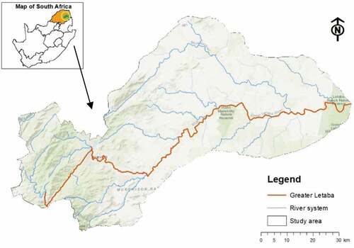
The study area is located within latitude: 23° 37ʹ 26.83ʹ’ S.036’S and longitude: 31° 5ʹ54.39ʹ’ E geographical co-ordinates (Figure 1). The study area falls within the tropical climate, with two distinct seasons. The area’s mean annual rainfall ranges from 612 mm during the wet season to 7 mm during the dry season. This seasonal variability influences rivers flows and water availability in the catchment which in turn impact nutrient distributions along river channels. The temperature ranges from 11°C in winter to 35°C in summer (DEAT 2001). This creates favorable growing conditions for water hyacinth as high temperatures enhance photosynthetic rates. For instance, shows that nutrient concentration and increased land surface temperatures influence the growth patterns and reproduction of water hyacinth species in open water bodies (Wilson, Holst, and Rees 2005). Water from the Greater Letaba river system serves a variety of services, including irrigation, domestic, as well as supporting aquatic life, especially in the upper part of the river. Water quality of the river has deteriorated, due to salinization and nutrient enrichment as a result of anthropogenic activities.

Figure 1. Locational map of the study area.

2.2. Data

2.2.1. Field data collection

Field data collection was done in the Greater Letaba river system, during the wet and dry season. Field data collection for dry and wet season coincided with acquisition day of Sentinel MSI images. Dry season data was collected from the 24^th to the 26^th of June 2017 where as for the wet season; it was from the 18^th to 20^th of October 2017. A Garmin Global Positioning System (GPS) was used to record the location of the water hyacinth. Additional data that was also collected included the dominant land cover types such as, bare land, built up, shrub-land, water, forest, riparian vegetation, and plantations. These land cover types were collected to enhance the classification process. A total of 765 points were randomly generated, using Hwath’s Analysis Tool embedded in ArcGIS 10.4 software. The field data were used for discrimination, classification using remote sensing images and validation of satellite-derived water hyacinth of the two seasons.

2.2.2. Remote sensing data

In this study, six cloudless tiles (ortho-images in UTM/WGS84 projection) of Sentinel-2 MSI remote sensing data covering the entire study area were used (Table 1). The images were downloaded from the online Sentinel Copernicus data hub. These images were acquired in top of atmosphere reflectance. The images were therefore atmospherically corrected, using the Dark Object Subtraction (DOS1) technique under Semi Automated Classification tool in QGIS version 2.18.03 software. Selection of this technique was based on its performance as reported in the literature (Pax-Lenney, Woodcock, and Macomber 2001; Liu et al. 2017; Thamaga and Dube 2018a). The technique applies the darkest pixel in the scene as an estimate of atmospheric path radiance (Lp) in all bands, assuming that, the atmosphere is homogenous across the entire scene (Matthews, Bernard, and Winter 2010). Further, the DOS1 technique works well in removing haze components caused by additive scattering from remote sensing data (Chavez 1989). However, the DOS1 technique has its own limitations for instance; the DOS1 assumes no atmospheric transmittance loss and no diffuse downward radiation at the surface (Chavez 1989; Tyagi and Bhosle 2011). Nevertheless, the technique has been used for correcting satellite images, which have resulted in better accuracies.

Table 1. Dry and wet season Sentinel-2 MSI acquisition dates used.

Season	Month	Scene detail
Dry	25 June 2017	RT_T36KTV_20170625T081348
		RT_T36KUU_20170625T080542
		RT_T36KTU_20170625T081227
		RT_T35KRP_20170625T074618
Wet	19 October 2017	RT_T35KQP_20171019T074941
		RT_T36KTU_20171019T074941
		RT_T36KTV_20171019T074941
		RT_T36KTU_20171019T074941
		RT_T35KRP_20171019T074941

For this study, 10 bands from Sentinel-2 images were used to achieve the aforementioned objective. These included the Blue, Green, and Red, NIR, Red-edge (1, 2 and 3), NIR-narrow and SWIR (1 and 2). Band 1 (coastal aerosol), 9 (water vapor) and 10 (SWIR – cirrus) were excluded for analysis, due to their spatial resolution (60 m) and relevance for the detection of atmospheric features (Drusch et al. 2012; Hagolle et al. 2015). The spectral bands within the NIR, Red-edge (1, 2 and 3), NIR-narrow and SWIR (1 and 2), with a spatial resolution of 20 m were also resampled to 10 m using the nearest neighbor resampling method in ArcGIS 10.4 software. This was done to ensure that all bands had a similar spatial resolution, for compatibility purposes and further analysis. Lastly, six scenes of Sentinel-2 images for each season were layered and mosaicked in ArcGIS 10.4 software. Figure 2 shows a summarised methodological framework followed in this study.

Figure 2. Methodological framework.

2.3. Data analysis

In this study, the Linear Discriminant Analysis (LDA) was employed to assess the spatial variations of water hyacinth in the Greater Letaba River system, for the wet and dry seasons. The LDA was run using sampled GPS points and associated Sentinel 2 variables (presented in Table 2) derived after extracting multi-values to points. LDA is a multivariate statistical classifier, which uses a discriminant or predictor function to classify land cover features into classes, using a measure of generalized squared distance (Dube et al. 2017). It converts reflected data derived from satellite images into components that explain the variations in reflectance among land cover types. The algorithm offers cross-validated results with Eigen value or variable scores that indicate the strength of a specific function in discriminating invasive water hyacinth from other dominant land cover classes. One of the assumptions of multivariate normality with equivalent covariance matrices is that the sample points are random, which was the case with land cover feature points used in this study. Besides, the algorithm applies the Box test (Chi-square and Fisher’s F asymptotic approximation), Wilks’s Lambda test (Rao’s approximation), Mahalanobis distances, and Kullback’s test to determine whether within-class covariance matrices were equal (Sibanda, Mutanga, and Rouget 2015; Sepuru and Dube 2018). The tests showed that there were significant differences (α = 0.05) between water hyacinth spectral responses and that of other land cover classes considered in this study. For statistical analysis, sampled GPS points were randomly split into training (70%) and testing (30%) sets (Adelabu et al. 2014; Adjorlolo et al. 2013; Sibanda, Mutanga, and Rouget 2015). Further, three analytically procedures were followed to discriminate water hyacinth from other land cover classes (Table 3). One-way Analysis of Variance (ANOVA) was used to test the spectral variation of water hyacinth from other land cover classes during wet and dry season. Three analytical sets of variables, namely: (i) spectral bands, (ii) spectral vegetation indices and (iii) integrated spectral bands and spectral vegetation indices were then used to derive accuracy assessment. Zonal statistical tool was also used to calculate area coverage of water hyacinth, between the two seasons.

Table 2. Sentinel-2 MSI spectral bands and vegetation indices used for this study.

Indices	Computation	References
Normalized Difference Vegetation Index (NDVI)	(NIR – Red)/(NIR + Red)	Tucker (1979)
Normalized Difference Water Index (NDWI)	(Green – NIR)/(Green + NIR)	McFeeters (1996)
Enhanced Vegetation Index (EVI)	2.5 * ((NIR – Red)/(1 + NIR + 6Red – 7.5Blue))	Huete et al. 1997
Simple Ratio Index (SRI)	(NIR/Red)	Jordan (1969)
Soil Adjusted Vegetation Index (SAVI)	((NIR – Red) * (1 + L))/(NIR2 + Red + L)	Huete (1988)
Greenness Index (GI)	Green/Red	Zarco-Tejeda et al. (2005)
Green Normalized Difference Vegetation Index (GNDVI)	(NIR – Green)/(NIR + Green)	Gitelson, Kaufman, and Merzlyak (1996)
Chlorophyll Index Green (Clgreen)	(NIR/Green) – 1	Gitelson et al. 2002
Atmospherically Resistant Vegetation Index (ARVI)	(NIR – (2*(Red – Blue)))/(NIR + (2*(NIR – Blue)))	Kaufman and Tanré 1992
Transformed Vegetation Index (TVI)	Squrt((NIR – Red)/(NIR + Red) + 0.5)	Deering et al. 1975
Optimized Soil-Adjusted Vegetation Index (OSAVI)	(NIR – Red)/(NIR + Red + 0.16)	Rondeaux, Steven, and Baret 1996
Renormalized difference vegetation index (RDVI)	Squrt((NDVI)(DVI))	Roujean and Breon 1995
Vegetation Greenness Index (VGI)	(Green – Red)/(Green + Red)	McFeeters (1996)
Normalised Green (NG)	Green/NIR + Red + Green	Sripada et al. 2006
Difference Vegetation Index (DVI)	NIR – Green	Tucker, 1979

Table 3. Sentinel-2 MSI experimental measures of accuracy assessment for water hyacinth.

Analysis	Data type	Spectral information
I	Spectral bands	Blue, Green, Red, Red edge(RE)-1, RE-2, RE-3, NIR, NIR narrow, SWIR-1 and SWIR-2
II	Vegetation Indices	NDVI, NDWI, EVI, SRI, SAVI, GI, GNDVI, Clgreen, ARVI, RVI, TVI, OSAVI, RDVI, VGI, NGI, DVI
III	SB + VIs	10 bands + 16 SVIs

2.4. Accuracy assessment

Accuracies in the form of cross tabulation matrices, using Millones and Pontius’ allocation were used to compute Overall Accuracy (OA), User Accuracy (UA), Producer Accuracy (PA) and kappa statistics from three analytical sets. We further used error bars to check the significance of the observed accuracies between different land cover types identified within the study area. Error bars were calculated using standard deviation.

3. Results

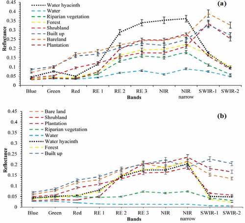
The results in Figure 3 show the averaged spectral profiles for water hyacinth and other key land cover classes of the study area during the wet and dry seasons. It was observed that, water hyacinth can be spectrally discriminated from other land cover types, i.e. bare land, built up, shrub-land, water, forest, riparian vegetation, and plantations mainly within the Red Edge (1, 2 and 3), NIR, NIR-narrow and SWIR (1 and 2) portions of the electromagnetic spectrum during wet and dry season.

Figure 3. Averaged spectral reflectance derived from Sentinel-2 MSI (a) wet season and (b) dry season.

3.1 Image analysis

3.1.1 Analysis I: water hyacinth classification accuracies derived from Sentinel-2 using raw spectral bands

Table 4 shows classification accuracies derived using spectral bands as independent data for dry and wet seasons. Spectral bands yielded an overall classification accuracy of 79.48% and 75.98% and kappa coefficients of 0.764 and of 0.724 for wet and dry seasons, respectively. Wet and dry season produced good classification accuracies derived, using spectral bands as a standalone variable, showed a slight difference of 3.50% (presented in Table 7) in terms of classification accuracy performance. Furthermore, spectral bands managed classify water hyacinth from other land cover classes with producer user and producer accuracies of water hyacinth ranging from 44% to 100%. Wet season water hyacinth classification results were achieved with a user accuracy of 87.18% and producer accuracy of 94.44%. On the other hand, high classification results were observed for the dry season water hyacinth mapping yielding user and producer accuracies of 84.62% and 66%, respectively. Other land cover classes were classified with high accuracies, for instance, Shrubland was classified with higher user accuracy of 93.33% and plantations with 73.91%.

Table 4. Confusion matrix derived using spectral bands for a) wet season and b) dry season showing the overall classification accuracy, user and producer accuracy for discrimination of water hyacinth amongst other land cover types derived using test data.

	Ground based observation
Predicted	(a)	Bareland	Built-up	Shrubland	Forest	Plantation	Riparian vegetation	Water	Water hyacinth	Total	User accuracy
	Bareland	30	0	3	0	0	0	0	0	33	90.91%
	Built-up	5	18	1	1	0	0	0	0	25	72.00%
	Shrubland	2	0	28	0	0	0	0	0	30	93.33%
	Forest	0	0	1	17	5	2	0	0	25	68.00%
	Plantation	0	0	0	5	17	2	0	1	25	68.00%
	Riparian vegetation	0	0	0	2	1	15	6	1	25	60.00%
	Water	0	0	0	2	0	2	23	0	27	85.19%
	Water hyacinth	0	0	0	3	0	2	0	34	39	87.18%
	Total	37	18	33	30	23	23	29	36	229	79.48%
	Producer accuracy	81.08%	100.00%	84.85%	56.67%	73.91%	65.22%	79.31%	94.44%
	Ground based observation
Predicted	(b)	Built-up	Forest	Plantation	Riparian vegetation	Shrubland	Water	Bareland	water hyacinth	Total	User accuracy
	Built-up	21	0	0	0	3	0	1	1	26	80.77%
	Forest	0	13	4	0	0	1	0	7	25	52.00%
	Plantation	1	1	20	0	1	1	0	1	25	80.00%
	Riparian vegetation	0	3	0	11	0	10	0	1	25	44.00%
	Shrubland	0	0	0	0	28	0	0	2	30	93.33%
	Water	0	0	0	1	0	21	0	5	27	77.78%
	Bareland	3	0	0	0	2	0	27	0	32	84.38%
	water hyacinth	0	3	2	0	0	1	0	33	39	84.62%
	Total	25	20	26	12	34	34	28	50	229	75.98%
	Producer accuracy	84.00%	65.00%	76.92%	91.67%	82.35%	61.76%	96.43%	66.00%

3.1.2 Analysis II: water hyacinth classification accuracies derived from Sentinel-2 using spectral vegetation indices

The use of spectral vegetation indices as independent dataset in discriminating and mapping water hyacinth yielded OA of 76.42% (kappa coefficient of 0.706) and 74.42% (kappa coefficient of 0.708) for wet and dry season, respectively (presented in Table 5). Comparatively, the OA dropped by 3.06% in wet season and by 1.56% in dry season (presented in Table 7) when compared to the use of spectral bands alone. UA and PA were derived with improved accuracies for the two seasons. As illustrated in Table 5, high UA (87.18% and 89.74%) and PA (94.44% and 66.04%), were observed for wet and dry season, respectively.

Table 5. Confusion matrix derived using vegetation indices for a) wet season and b) dry season showing the overall classification accuracy, user and producer accuracy for discrimination of water hyacinth amongst other land cover types derived using test data.

	Ground based observation
Predicted	(a)	Bareland	Built-up	Shrubland	Forest	Plantation	Riparian vegetation	Water	Water hyacinth	Total	User accuracy
	Bareland	26	3	4	0	0	0	0	0	33	78.79%
	Built-up	9	16	0	0	0	0	0	0	25	64.00%
	Shrubland	0	1	29	0	0	0	0	0	30	96.67%
	Forest	0	0	2	19	4	0	0	0	25	76.00%
	Plantation	0	0	0	6	18	0	0	1	25	72.00%
	Riparian vegetation	0	0	0	5	0	16	3	1	25	64.00%
	Water	0	0	0	1	0	9	17	0	27	62.96%
	Water hyacinth	0	0	0	1	0	4	0	34	39	87.18%
	Total	35	20	35	32	22	29	20	36	229	76.42%
	Producer accuracy	74.29%	80.00%	82.86%	59.38%	81.82%	55.17%	85.00%	94.44%
	Ground based observation
Predicted	(b)	Built-up	Forest	Plantation	Riparian vegetation	Shrubland	Water	Bareland	water hyacinth	Total	User accuracy
	Built-up	21	0	0	0	3	0	2	0	26	80.77%
	Forest	0	12	3	0	1	0	0	9	25	48.00%
	Plantation	2	5	14	0	0	0	0	4	25	56.00%
	Riparian vegetation	0	3	0	18	0	4	0	0	25	72.00%
	Shrubland	4	0	0	0	24	0	0	2	30	80.00%
	Water	0	1	0	4	0	19	0	3	27	70.37%
	Bareland	2	0	0	0	2	0	28	0	32	87.50%
	water hyacinth	0	3	1	0	0	0	0	35	39	89.74%
	Total	29	24	18	22	30	23	30	53	229	74.67%
	Producer accuracy	72.41%	50.00%	77.78%	81.82%	80.00%	82.61%	93.33%	66.04%

Table 6. Confusion matrix derived using combined spectral bands and vegetation indices for a) wet season and b) dry season showing the overall classification accuracy, user and producer accuracy for discrimination of water hyacinth amongst other land cover types derived using test data.

	Ground based observation
Predicted	(a)	Bareland	Built-up	Shrubland	Forest	Plantation	Riparian vegetation	Water	Water hyacinth	Total	User accuracy
	Bareland	31	0	2	0	0	0	0	0	33	93.94%
	Built-up	6	19	0	0	0	0	0	0	25	76.00%
	Shrubland	0	1	29	0	0	0	0	0	30	96.67%
	Forest	0	0	1	18	4	2	0	0	25	72.00%
	Plantation	0	0	0	5	19	0	0	1	25	76.00%
	Riparian vegetation	0	0	0	4	0	17	3	1	25	68.00%
	Water	0	0	0	2	0	6	19	0	27	70.37%
	Water hyacinth	0	0	0	3	1	2	0	33	39	84.62%
	Total	37	20	32	32	24	27	22	35	229	80.79%
	Producer accuracy	83.78%	95.00%	90.63%	56.25%	79.17%	62.96%	86.36%	94.29%
	Ground based observation
Predicted	(b)	Built-up	Forest	Plantation	Riparian vegetation	Shrubland	Water	Bareland	water hyacinth	Total	User accuracy
	Built-up	21	0	0	0	3	0	1	1	26	80.77%
	Forest	0	12	3	0	1	0	0	9	25	48.00%
	Plantation	0	5	15	0	2	0	0	3	25	60.00%
	Riparian vegetation	0	1	0	22	0	2	0	0	25	88.00%
	Shrubland	0	0	0	0	30	0	0	0	30	100.00%
	Water	0	1	0	4	0	19	0	3	27	70.37%
	Bareland	3	0	0	0	2	0	27	0	32	84.38%
	Water hyacinth	0	3	1	0	0	0	0	35	39	89.74%
	Total	24	22	19	26	38	21	28	51	229	79.04%
	Producer accuracy	87.50%	54.55%	78.95%	84.62%	78.95%	90.48%	96.43%	68.63%

Table 7. Magnitude of classification accuracies of wet and dry season derived from Sentinel-2 MSI.

			Deviations in terms of accuracy (%)
Season	Parameter	Accuracy (%)	I	II	III
wet season	Bands	79.48	-	3.06	1.31
	VIs	76.42	3.06	-	4.37
	Bands + VIs	80.79	1.31	4.37	-
Dry season	Bands	75.98	-	1.56	3.06
	VIs	74.42	1.56	-	4.62
	Bands + VIs	79.04	3.06	4.62	-

*I: Spectral bands, II: Vegetation indices and III: Combined spectral bands and vegetation.

3.1.3 Analysis III: water hyacinth classification accuracies derived from Sentinel-2 using raw spectral bands and spectral vegetation indices

The use of integrated dataset (spectral bands and vegetation indices) resulted in further improvement in the OA. The integrated dataset managed to achieve an OA of 80.79% (kappa coefficient of 0.780) during wet season compared to 79.04% (kappa coefficient of 0.759) in dry season (Table 6). Similar results were observed for the PA and UA. In this case, water hyacinth was classified with high UA and PA of 84.62% and 94.29% in wet season, as well as 89.74% and 68.63% in dry season, respectively. Overall, analysis III yielded high UA and PA from when compared to analysis II and I. Overall, the classification results were significantly different demonstrating the value added by data integration in water hyacinth mapping.

The overall classification accuracies illustrated in Figure 4 were achieved by using spectral bands (Analysis I), vegetation indices (Analysis II), as well as integrated (spectral bands and vegetation indices) dataset (Analysis III) derived from multi-seasonal Sentinel-2 MSI. Analysis of variance (ANOVA) showed that there was a significant difference amongst the accuracies derived from the three experiments, i.e. (t = 1.86, p < 0.001) analysis I, analysis II (t = 1.761, p < 0.435) and analysis III (t = 1.710, p < 0.472).

Figure 4. Combined spectral bands and vegetation indices overall classification accuracies derived during wet and dry season from Sentinel-2 MSI.

3.2 Seasonal mapping of the spatial distribution of water hyacinth

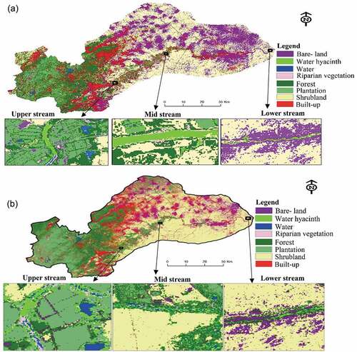
The derived water hyacinth spatial distribution maps for dry and wet seasons are demonstrated in Figure 5. Overall, Sentinel-2 showed the capability of detecting and mapping seasonal distribution of water hyacinth. In the lower, mid and upper parts of the river, it can be seen that there was a high coverage of water hyacinth detected in summer (wet season), than in dry season. For instance, in the wet season, water hyacinth covered a surface area of 68.82%, whereas in the dry season, 28.34% coverage was detected, with a deviation of 40.48%.

Figure 5. Seasonal maps derived using Sentinel-2 MSI (a) wet season and (b) dry season.

4. Discussion

4.1. Characterization of water hyacinth Sentinel 2 using Sentinel 2

The study was aimed at understanding the seasonal distribution patterns of water hyacinth (Eichhornia crassipes) using Sentinel-2 MSI satellite data, in the Greater Letaba river system in Tzaneen, South Africa. Results from this study, demonstrated that Sentinel 2 data can detect and map the spatial distribution of water hyacinth in narrow river channels. The integration of spectral bands and vegetation indices showed the highest capability of detecting and mapping the temporal distribution of water hyacinth in freshwater system with an OA of 80.79% during the wet season and 79.04% in the dry season. The unique performance of Sentinel 2 data has been demonstrated and reported in other studies with particular emphasis on vegetation mapping, i.e. estimation of plant biophysical parameters, biomass, crop and fire monitoring as well as land cover mapping (Sonobe et al. 2017; Forkuor et al. 2018; Mallinis, Mitsopoulos, and Chrysafi 2018; Sibanda et al. 2019). Despite its wider use in vegetation monitoring its utility in water resources applications has remained rudimentary. This work, therefore, for the first time underlines the importance of the recently launched Sentinel 2 data in detecting and mapping aquatic weeds such as water hyacinth in open-waterbodies occurring in very narrow river channels.

Findings of this work also provide new insights into the potential of new generation sensors like Sentinel 2, with improved spatial, temporal and spectral characteristics in water resources monitoring ungauged and very narrow or small river channels. Sentinel imagery provide more accurate and unique information on the spatial distribution and configuration of water hyacinth, a previous daunting task with broadband multispectral sensors especially in smaller and narrow water bodies (Shekede, Kusangaya, and Schmidt 2008; Ndungu et al. 2013; Dube, Gumindoga, and Chawira 2014; Dube et al. 2017). This breakthrough provides critical baseline information required in assessing the status of river water courses and determining affected areas and possible vulnerable areas. Also, this information is fundamental to aquatic specialists; water resource-related managers, decision-makers, and other interested stakeholders, especially in data scarce areas with limited network of field monitoring frameworks in place. Besides, seasonal mapping of these species gives a better view in understanding its spatial distribution and configuration required for frequent monitoring, assessment of infestation levels, sustainable remedial, eradication and effective management practices (Thiemann and Kaufmann 2002; Shekede, Kusangaya, and Schmidt 2008; Ndungu et al. 2013; Dube et al. 2017; Vaz et al. 2018).

Further, the use of spectral bands and vegetation indices as independent classification dataset showed slightly weaker water hyacinth classification results for both the dry and the wet season. This result concurs with the work by Thamaga and Dube (2018a), Sibanda et al. (2019) and, Shoko and Mutanga (2017) who observed that the integration of raw band information and vegetation indices. For instance, Sibanda et al. (2019) using Sentinel-2 derived Red Edge bands estimated leaf area index and canopy storage capacity for wattle invasive plant species with a high overall accuracy (RMSEP of 0.507 m² · m⁻², a relative RMSE of prediction of 11.3% and R² of 0.91 for LAI). Thamaga and Dube (2018a) confirmed the superior nature of Sentinel over Landsat in mapping water hyacinth, producing an overall accuracy of 77.56% using combined dataset. Immitzer, Vuolo, and Atzberger (2016) used Sentinel data based on the object-oriented random forest algorithm in Central Europe to mapped forest types and the study obtained an overall classification accuracy of 66.2%. This result illustrates the importance of integrating multispectral derivatives in detecting the invasive water hyacinth across seasons. The slightly weaker performance from the use of spectral or vegetation indices as standalone model dataset in mapping water hyacinth can be attributed to saturation problems or spectral mixing (Dube et al. 2014; Dube and Mutanga 2015). This can also be attributed by the presence of algae blooms in water, which influences the reflectance in the NIR and SWIR portions of the electromagnetic spectrum than in the red, blue and green portions (Muchini et al. 2018).

4.2. The seasonal dynamics of water hyacinth distribution within the river system

The results of the study showed significant variability in the area covered by water hyacinth between the dry and the wet seasons. During the wet season, water hyacinth covered approximately 68.82% and 28.34% of the monitored area in dry season. The concentration varied across the lower, mid and upper part of the river system. These findings are similar to those of Dube et al. (2017) who observed high water hyacinth concentrations during wet season than dry season in Lake Manyame and Lake Chivero. High concentrations during wet season can be attributed to improved growth rates enhanced by nutrient supplies from surrounding farming areas due to enhanced river flows and runoff (Shekede, Kusangaya, and Schmidt 2008). Further, warm temperatures and flow dynamics fuel the spatio-temporal distribution of this species in freshwater especially during the wet season (Thornton et al. 2014; Brierley and Kingsford 2009). Adams et al. (2002); Mireri (2005); Téllez et al. (2008); Waltham and Fixler (2017) observed significant increases in the nutrient concentrations and raising temperatures cause eutrophication which accelerates water hyacinth infestation on the lake during the wet season. Less water hyacinth coverage during the dry season can be attributed to reduced runoff or river flows during in this period as most of the rivers are ephemeral, only flow when it rains and this hinders the growth due to limited nutrient supply. During this time of the season, there is less runoff and nutrient recharge in the river system which result in less movement of nutrients which supports or favors growth of species invasion. Mitsch (1985) noted that in water bodies with low nutrient levels the probability of the water hyacinth growth is likely to be out-competed by other aquatic species exists within water channels.

Further, seasonal variability in temporal distribution of water hyacinth showed that, the dry season had a deviation of ±3.50% in terms of accuracy when compared to wet season results. The accuracy difference between two seasonal images can be attributed to the variability in nutrient load and weather conditions (Téllez et al. 2008; Waltham and Fixler 2017). Extreme temperatures as a result of weather changes and flow dynamics fuel the spatio-temporal distribution of this species in freshwater (Thornton et al. 2014; Brierley and Kingsford 2009). These results thus provides a better view in understanding its spatial distribution and configuration required for establishing sustainable remedial, eradication and effective management practices. This finding agrees with several studies that have demonstrated the potential of the 10 m spatial resolution Sentinel 2 data in tree species mapping in natural ecosystems (Immitzer, Vuolo, and Atzberger 2016; Sibanda et al. 2019). Mat-coverage of water hyacinth negatively impact freshwater ecosystem and water due to high to evapotranspiration (Mitchell 1985; Shekede, Kusangaya, and Schmidt 2008; Mironga, Mathooko, and Onywere 2014). Osmond and Petroeschhevsky (2013) mentioned that water loss can reach three times greater than the natural evaporation rate of water surface that does not have water hyacinth. Stan et al. (2016) reported that evaporation of open water is averaged 4.3 mm day⁻¹ and evapotranspiration of aquatic plants an average of 7.8 mm day⁻¹. Less amount of water hyacinth during dry season depicted by Sentinel 2 MSI illustrated is due to unfavorable climatic conditions. Therefore, this result can be used in modeling water loss due to invasive water hyacinth presence in rivers and can help in prioritization of the eradication endeavors.

The high accuracies observed in this finding can also be attributed to the presence of unique and strategically position spectral bands found in Sentinel 2 data. For example, it can be observed that the red edge bands B5, 6 and 7, NIR, NIR-narrow and SWIR (1 and 2) portions of the electromagnetic spectrum demonstrated a unique capability in discriminating water hyacinth from other land cover types considered in this study. This finding concurs with previous studies which highlighted the capability of using Sentinel-2 MSI in vegetation mapping-related studies (Sibanda, Mutanga, and Rouget 2016; Dube et al. 2017; Shoko and Mutanga 2017, Forkuor et al. 2017). Most of these attributed the unique results to the presence of most strategic region of red edge bands (B5, 6 and 7) which are critical for mapping vegetation properties (Sibanda, Mutanga, and Rouget 2015). The red edge bands have been reported to be more sensitive to subtle plant biophysical parameters hence the ability to detect water hyacinth from other land cover classes with high accuracy. It could be due to this reason that the inclusion of the red edge bands resulted in high water hyacinth classification accuracies. In a related study, Sibanda et al. (2019) and Shoko et al. (2018) illustrated that the red-edge correlated strongly with biophysical parameters like LAI.

4.3. Implications of remote sensing water hyacinth

Growing of water resource scarcity and their security, in changing environment, has long been recognized and remains a challenge particularly in African. However, water quality management is considered challenging due to complexities of water environments, in connection to their contributing tributaries within the watersheds. Regardless of extensive knowledge on the causes and implications of the proliferation of water hyacinth in freshwater ecosystems, the accurate and reliable information on their spatial distribution, configuration, as well as propagation rates remains a challenge in data scarce regions such as sub-Saharan Africa. Remote sensing of inland waters has faced challenges in the retrieval of physical and biogeochemical properties. However, findings of this study suggest a shift towards implementation of cutting edge remote sensing technologies in monitoring and management of freshwater ecosystems. This information is critical for development of effective aquatic weed control and eradication programs, especially in resource scarce regions. The results demonstrate that water hyacinth can be better controlled during the dry season when its concentration has dwindled as this would help to minimize the costs of its removal or control.

5. Conclusions

The present study focused on mapping the spatio-temporal distribution of water hyacinth in the river system during wet and dry seasons, using Sentinel-2 MSI satellite data. The findings of this study showed that Sentinel-2 MSI satellite provide new opportunities for mapping and monitoring of seasonal distribution of water hyacinth in open water systems.

We conclude that:

• Large spatial coverage of water hyacinth was detected during the wet season, compared to the dry season.

• Areas of the river system proximity to irrigation systems and residential were associated with more water hyacinth.

• Sentinel-2 MSI with improved spectral and spatial resolution managed to detect and map the seasonal distribution and spatial dynamics of water hyacinth in a river system.

Overall, the findings of this work provide new insights and critical on the usefulness of new generation sensors in monitoring aquatic water weeds and such findings can be key in decision-making and policy development and draw remedial measures. It is however, important to note that any current image classification technique (including the DA) always produce “mixed classes” (error). This is due to the presence of many natural fuzzy objects, which are very difficult and even impossible to distinguish automatically and straightforward. There is, therefore, need to treat these findings with caution and further research to focus only on water hyacinth and establish whether this can help to minimize classification error.

Highlights

• Growth rate of water hyacinth is higher in wet season than in dry season

• Understanding of temporal distribution of water hyacinth is limited

• There is a need for continuous monitoring of aquatic species in a river system using non-commercial sensors

Acknowledgements

Authors would like to express their gratitude to Risk and Vulnerability Science Centre (RVSC) for funding this project. Furthermore, authors are appreciative to the Sentinel Copernicus data hub for the provision of Sentinel-2 MSI images with no cost attached. We also like to express gratitude to Mr Sepuru T.K. and Mr Dhau I. for assisting with field data collection.

Disclosure statement

No potential conflict of interest was reported by the authors.

References

- Adams, C. S, R. R. Boar, D. S. Hubble, M. Gikungu, D. M. Harper, and P. Hickley. 2002. “The Dynamics and Ecology of Exotic Tropical Plants in Floating Plant Mats: Lake Naivasha, Kenya.” Hydrobiologia 488: 115–122. doi:10.1023/A:1023322430005.
- Adelabu, S., O. Mutanga, E. Adam, and R. Sebego. 2014. “Spectral Discrimination of Insect Defoliation Levels in Mopane Woodland Using Hyperspectral Data.” IEEE Journal of Selected Topics Applied Earth Observations Remote Sensing 7: 177–185.
- Adjorlolo, C., O. Mutanga, M. A. Cho, and R. Ismail. 2013. “Spectral Resampling Based on User-Defined Inter-band Correlation Filter: C3 and C4 Grass Species Classification.” International Journal of Applied Earth Observation and Geoinformation 21: 535–544. doi:10.1016/j.jag.2012.07.011.
- Albright, T. P., T. G. Moorhouse, and T. J. McNabb. 2004. “The Rise and Fall of Water Hyacinth in Lake Victoria and the Kagera River Basin, 1989-2001.” Journal of Aquatic Plant Management 42: 79–84.
- Bradley, B. A., and J. F. Mustard. 2006. “Characterizing the Landscape Dynamics of an Invasive Plant and Risk of Invasion Using Remote Sensing.” Ecological Applications 16: 1132–1147. doi:10.1890/1051-0761(2006)016[1132:CTLDOA]2.0.CO;2.
- Brierley, A. S., and M. L. Kingsford. 2009. “Impact of Climate Change on Marine Organisms and Ecosystems.” Current Biology 19 (14): R602–R614. doi:10.1016/j.cub.2009.05.046.
- Campos-Taberner, M., F. J. García-Haro, G. Camps-Valls, F. N. Grau-Muedra, M. Boscheti, and M. Boscheti. 2016. “Multitemporal and Multiresolution Leaf Area Index Retrieval for Operational Local Rice Crop Monitoring.” Remote Sensing of Environment 187: 102–118. doi:10.1016/j.rse.2016.10.009.
- Chandra, G., A. Ghosh, D. Biswas, and S. Chatterjee. 2006. “Host Plant Preference of Mansonia Mosquitoes.” Journal of Aquatic Plant Management 44: 142–144.
- Chavez, P., Jr. 1989. “Radiometric Calibration of Landsat Thematic Mapper Multispectral Images.” Photogrammetric Engineering and Remote Sensing 55 (9): 1285–1294.
- Cheruiyot, E. K., C. Mito, M. Menenti, B. Gorte, R. Koenders, and N. Aksim. 2014. “Evaluating MERIS-Based Aquatic Vegetation Mapping in Lake Victoria.” Remote Sensing 6: 7762–7782.
- Clayton, J. S., and P. D. Champion. 2006. “Risk Assessment Method for Submerged Weeds in New Zealand Hydroelectric Lakes.” Hydrobiologia 570: 183–188. doi:10.1007/s10750-006-0179-z.
- DEAT. 2001. “State of the Rivers Report.” Accessed 20 February 2017. http://soer.deat.gov.za/dm_documents/LimpopoLLtf4tA.pdf
- Deering, D. W., J. W. Rouse, R. H. Haas, and J. A. Schell. 1975. “Measuring ‘Forage Production’ of Grazing Units from Landsat MSS Data.” Proceedings of the 10th International Symposium on Remote Sensing of Environment II, 1169–1178.
- Drusch, M., U. Del Bello, S. Carlier, O. Colin, V. Fernandez, F. Gascon, B. Hoersch, C. Isola, P. Labertini, and P. Martimort. 2012. “Sentinel-2: ESA’s Optical High-resolution Mission for GMES Operational Services.” Remote Sensing of Environment 120: 25–36. doi:10.1016/j.rse.2011.11.026.
- Dube, T., and O. Mutanga. 2015. “Evaluating the Utility of the Medium-spatial Resolution Landsat 8 Multispectral Sensor in Quantifying Aboveground Biomass in uMgeni Catchment, South Africa.” ISPRS Journal of Photogrammetry and Remote Sensing 101: 36–46. doi:10.1016/j.isprsjprs.2014.11.001.
- Dube, T., O. Mutanga, A. Elhadi, and R. Ismail. 2014. “Intra-And-inter Species Biomass Prediction in a Plantation Forest: Testing the Utility of High Spatial Resolution Spaceborne Multispectral Rapideye Sensor and Advanced Machine Learning Algorithms.” Sensors 14 (8): 15348–15370. doi:10.3390/s140815348.
- Dube, T., O. Mutanga, K. E. Seutloali, and C. Shoko. 2015. “Water Quality Monitoring in sub-Saharan African Lakes: A Review of Remote Sensing Applications.” African Journal of Aquatic Science 40 (1): 1–7. doi:10.2989/16085914.2015.1014994.
- Dube, T., O. Mutanga, M. Sibanda, V. Bangamwabo, and C. Shoko. 2017. “Testing the Detection and Discrimination Potential of the New Landsat 8 Satellite Data on the Challenging Water Hyacinth (eichhornia Crassipes) in Freshwater Ecosystems.” Applied Geography 84: 11–22. doi:10.1016/j.apgeog.2017.04.005.
- Dube, T., W. Gumindoga, and M. Chawira. 2014. “Detection of Land Cover Changes around Lake Mutirikwi, Zimbabwe, Based on Traditional Remote Sensing Image Classification Techniques.” Africa Journal Aquatic Science 39 (1): 89–95. doi:10.2989/16085914.2013.870068.
- Everitt, J. H., C. Yang, D. E. Escobar, C. F. Webster, R. I. Lornard, and M. R. Davis. 1999. “Using Remote Sensing and Spatial Information Technologies to Detect and Map Two Aquatic Macrophytes.” Journal of Aquatic Plant Management 37: 71–80.
- Forkuor, G., K. Dimobe, I. Serme, and J. E. Tondoh. 2018. “Landsat-8 Vs. Sentinel-2: Examining the Added Value of Sentinel-2’s Red-edge Bands to Land-use and Land-cover Mapping in Burkina Faso.” GIScience & Remote Sensing 55 (3): 331–354. doi:10.1080/15481603.2017.1370169.
- Forkuor, G., O. K. L. Hounkpatin, G. Welp, and M. Thiel, 2017. “High Resolution Mapping of Soil Properties Using Remote Sensing Variables in South-western Burkina Faso: A Comparison of Machine Learning and Multiple Linear Regression Models.” PlusOne doi:10.1371/journal.pone.0170478
- Fusilli, L., M. O. Collins, G. Laneve, A. Palombo, S. Pignatti, and F. Santini. 2013. “Assessment of the Abnormal Growth of Floating Macrophytes in Winam Gulf (kenya) by Using MODIS Imagery Time Series.” International Journal Application of Earth Observation and Geoinformation 20: 33–41. doi:10.1016/j.jag.2011.09.002.
- Getsinger, K. D., E. D. Dibble, J. H. Rodgers, and D. F. Spencer. 2014. Benefits of Controlling Nuisance Aquatic Plants and Algae in the United States, 12. Ames: Council on Agricultural Science and Technology.
- Gitelson, A. A., Y. J. Kaufman, and M. N. Merzlyak. 1996. “Use of a Green Channel in Remote Sensing of Global Vegetation from EOS-MODIS.” Remote Sensing of the Environment 58: 289–298. doi:10.1016/S0034-4257(96)00072-7.
- Gitelson, A. A., Y. J. Kaufman, R. Stark, and D. Rundquist. 2002. “Novel Algorithms for Remote Sensing Estimation of Vegetation Fraction.” Remote Sensing of Environment 80: 76–87.
- Hagolle, O., S. Sylvander, M. Huc, M. Claverie, D. Clesse, C. Dechoz, V. Lonjou, and V. Poulain. 2015. “SPOT-4 (take 5): Simulation of Sentinel-2 Time Series on 45 Large Sites.” Remote Sensing 7 (9): 12242–12264. doi:10.3390/rs70912242.
- Halstead, J. M., J. Michaud, and S. H. Hallas-Burt. 2003. “Hedonic Analysis of Effects of a Non-native Invader (myriophyllum Heterophyllum) on New Hampshire (USA) Lakefront Properties.” Environmental Management 32: 391–398. doi:10.1007/s00267-003-3023-5.
- Harmel, T., M. Chami, T. Tormos, N. Reynaud, and P. Danis. 2018. “Sunglint Correction of the Multi-Spectral Instrument (msi)-sentinel-2 Imagery over Inland and Sea Waters from SWIR Bands.” Remote Sensing of Environment 204: 308–321. doi:10.1016/j.rse.2017.10.022.
- Hestir, E. L., S. Khanna, M. E. Andrew, M. J. Santos, J. H. Viers, and J. A. Greenberg. 2008. “Identification of Invasive Vegetation Using Hyperspectral Remote Sensing in the California Delta Ecosystem.” Remote Sensing of Environment 112: 4034–4047. doi:10.1016/j.rse.2008.01.022.
- Hill, M. P., and J. Coetzee. 2017. “The Biological Control of Aquatic Weeds in South Africa: Current Status and Future Challenges.” Bothalia - African Biodiversity and Conservation 47 (2): a2152.
- Holm, L. G., D. L. Plucknett, J. V. Pancho, and J. P. Herberger. 1991. The World’s Worst Weeds: Distribution and Biology. Malabar, FL: Kreiger.
- Holm, L. G., L. W. Weldon, and R. D. van Blackburn. 1969. “Aquatic Weeds.” Science 166: 699–709. doi:10.1126/science.166.3906.699.
- Huete, A., H. Liu, K. V. Batchily, and W. van Leeuwen. 1997. “A Comparison of Vegetation Indices over a Global Set of TM Images for EOS-MODIS.” Remote Sensing of the Environment 59: 440–451. doi:10.1016/S0034-4257(96)00112-5.
- Huete, A. R. 1988. “A Soil-Adjusted Vegetation Index (SAVI).” Remote Sensing of the Environment 25: 295–309. doi:10.1016/0034-4257(88)90106-X.
- Immitzer, M., F. Vuolo, and C. Atzberger. 2016. “First Experience with Sentinel-2 Data for Crop and Tree Species Classifications in Central Europe.” Remote Sensing 8 (3): 166. doi:10.3390/rs8030166.
- Jordan, C. F. 1969. “Derivation of Leaf-area Index from Quality of Light on the Forest Floor.” Ecology 50: 663–666. doi:10.2307/1936256.
- Kaufman, Y. J., and D. Tanré. 1992. “Atmospherically Resistant Vegetation Index (ARVI) for EOS-MODIS.” IEEE Transactions on Geoscience and Remote Sensing 30 (2): 261–270. doi:10.1109/36.134076.
- Khanna, S., M. J. Santos, S. L. Ustin, and P. J. Haverkamp. 2011. “An Integrated Approach to a Biophysiologically Based Classification of Floating Aquatic Macrophytes.” International Journal of Remote Sensing 32 (4): 1067–1094. doi:10.1080/01431160903505328.
- Law, R. 2007. “Fisheries-Induced Evolution: Present Status and Future Directions.” Marine Ecology Progress Series 335: 271–277. doi:10.3354/meps335271.
- Liu, Q., X. Gao, L. He, and W. Lu. 2017. “Haze Removal for a Single Visible Remote Sensing Image.” Signal Processing 137: 33–43. doi:10.1016/j.sigpro.2017.01.036.
- Lodge, D. M., S. L. Williams, H. MacIsaac, K. Hayes, B. Leung, S. Reichard, R. N. Mack, et al. 2006. “Biological Invasions: Recommendations for U.S. Policy and Management.” Ecological Applications 16: 2035–2054.
- Luo, J., H. Duan, R. Ma, X. Jin, F. Li, W. Hu, K. Shi, and W. Huang. 2017. “Mapping Species of Submerged Aquatic Vegetation with Multi-seasonal Satellite Images and considering Life History Information.” International Journal of Applied Earth Observation and Geoinformation 57: 154–165. doi:10.1016/j.jag.2016.11.007.
- Malik, A. 2007. “Environmental Challenge Vis a Vis Opportunity: The Case of Water Hyacinth.” Environment International 33: 122–138. doi:10.1016/j.envint.2006.08.004.
- Mallinis, G., I. Mitsopoulos, and I. Chrysafi. 2018. “Evaluating and Comparing Sentinel 2A and Landsat-8 Operational Land Imager (OLI) Spectral Indices for Estimating Fire Severity in a Mediterranean Pine Ecosystem of Greece.” GIScience & Remote Sensing 55 (1): 1–18. doi:10.1080/15481603.2017.1354803.
- Matthews, M. W., S. Bernard, and K. Winter. 2010. “Remote Sensing of Cyanobacteria Dominant Algal Blooms and Water Quality Parameters in Zeekoevlei, a Small Hypertrophic Lake, Using MERIS.” Remote Sensing of Environment 114 (9): 2070–2087. doi:10.1016/j.rse.2010.04.013.
- McFeeters, S. K. 1996. “The Use of the Normalized Difference Water Index (NDWI) in the Delineation of Open Water Features.” International Journal of Remote Sensing 17: 1425–1432. doi:10.1080/01431169608948714.
- Minakawa, N., G. Sonye, G. Dida, K. Futami, and S. Kaneko. 2008. “Recent Reduction in the Water Level of Lake Victoria Has Created More Habitats for Anopheles Funestus.” Malaria Journal 7: 119. doi:10.1186/1475-2875-7-129.
- Mireri, C. 2005. “Challenges Facing the Conservation of Lake Naivasha, Kenya.” Topics of Integrated Watershed Management-proceedings, 3.
- Mironga, J. M., J. M. Mathooko, and S. M. Onywere. 2014. “Effects of Spreading Patterns of Water Hyacinth (eichhornia Crassipes) on Zooplankton Population in Lake Naivasha, Kenya.” International Journal of Sustainable Development 3 (10): 1971–1987.
- Mitchell, D. S. 1985. “Surface-floating Aquatic Macrophytes.” In The Ecology and Management of African Wetland Vegetation, edited by P. Denny, 109–124. Dordrecht: Dr. W. Junk Publishers.
- Molinos, J. G., M. Viana, M. Brennan, and I. Donohue. 2015. “Importance of Long-Term Cycles for Predicting Water Level Dynamics in Natural Lakes.” Plus One 10 (3): e0119253. doi:10.1371/journal.pone.0119253.
- Muchini, R., W. Gumindoga, S. Togarepi, T. P. Masrira, and T. Dube. 2018. “Near Real Time Water Quality Monitoring of Chivero and Manyame Lakes of Zimbambwe.” In Copernicus Publication on Behalf of the International Association of Hydrological Science, 85–92. Vol. 378.
- Ndimele, P. E., C. A. Kumolu-Johnson, and M. A. Anetekhai. 2011. “The Invasive Aquatic Macrophyte, Water Hyacinth {eichhornia Crassipes (mart.) Solm-Laubach: Pontederiaceae}: Problems and Prospects.” Research Journal of Environmental Sciences 5: 509–520. doi:10.3923/rjes.2011.509.520.
- Ndungu, J., D. C. M. Augustijn, S. J. M. H. Hulscher, N. Kitaka, and J. Mathooko. 2013. “Spatio-temporal Variations in the Trophic Status of Lake Naivasha, Kenya.” Lakes and Reservoirs Science, Policy and Management for Sustainable Use 18 (4): 317–328.
- Osmond, R., and A. Petroeschhevsky. 2013. “Water Hyacinth Control Modules Control Options for Water Hyacinth (Eichhornia crassipes) in Australia.” Australia: New South Wales Department of Primary Industries. Retrieved from https://www.dpi.nsw.gov.au/__data/assets/pdf_file/0005/505706/waterhyacinth-control-modules-full-accessible.pdf
- Palmer, S. C. J., T. Kutser, and P. D. Hunter. 2015. “Remote Sensing of Inland Waters Challenges, Progress and Future Directions.” Remote Sensing of Environment 157: 1–8. doi:10.1016/j.rse.2014.09.021.
- Pax-Lenney, M., C. E. Woodcock, and S. A. Macomber. 2001. “Forest Mapping with Generalized Classifier and Landsat TM Data.” Remote Sensing of Environment 241–250. doi:10.1016/S0034-4257(01)00208-5.
- Penfound, W. T., and T. T. Earle. 1948. “The Biology of the Water Hyacinth.” Ecological Monographs 18: 447–472. doi:10.2307/1948585.
- Pimentel, D., L. Lach, R. Zungiga, and D. Morrison. 2005. “Update on the Environmental and Economic Costs Associated with Alien Invasive Species in the United States.” Ecological Economics 52: 273–288. doi:10.1016/j.ecolecon.2004.10.002.
- Pyšek, P., and D. M. Richardson. 2010. “Invasive Species, Environmental Change and Management, and Health.” Annual Review of Environment and Resources 35: 1. doi:10.1146/annurev-environ-033009-095548.
- Roijackers, R., S. Szabo, and M. Scheffer. 2004. “Experimental Analysis of the Competition between Algae and Duckweed.” Archiv Fur Hydrobilogie 160: 401–412. doi:10.1127/0003-9136/2004/0160-0401.
- Rondeaux, G., M. Steven, and F. Baret. 1996. “Optimization of Soil-adjusted Vegetation Indices.” Remote Sensing of Environment 55: 95–107. doi:10.1016/0034-4257(95)00186-7.
- Roujean, J. L. and F. M. Breon. 1995. “Estimating Par Absorbed by Vegetation from Bidirectional Reflectance Measurements.” Remote Sensing of Environment 51: 375–384. doi:10.1016/0034-4257(94)00114-3.
- Sepuru, T. K., and T. Dube. 2018. “Understanding the Spatial Distribution of Eroded Areas in the Former Rural Homelands of South Africa: Comparative Evidence from Two New Non-commercial Multispectral Sensors.” International Journal of Applied Earth Observations and Geoinformation 69: 119–132. doi:10.1016/j.jag.2018.02.020.
- Shekede, M., S. Kusangaya, and K. Schmidt. 2008. “Spatio-temporal Variations of Aquatic Weed Abundance and Coverage in Lake Chivero, Zimbabwe.” Physics and Chemical of the Earth Parts A/B/C 33: 714–721. doi:10.1016/j.pce.2008.06.052.
- Shoko, C., and O. Mutanga. 2017. “Examining the Strength of the Newly-launched Sentinel 2 MSI Sensor in Detecting and Discriminating Subtle Differences between C3 and C4 Grass Species.” ISPRS Journal of Photogrammetry and Remote Sensing 129: 32–40. doi:10.1016/j.isprsjprs.2017.04.016.
- Shoko, C., O. Mutanga, T. Dube, and R. Slotow. 2018. “Characterizing The Spatio-temporal Variations Of C3 and C4 Dominated Grasslands Aboveground Biomass in The Drakensberg, South Africa.” International Journal Of Applied Earth Observation and Geoinformation 68: 51 – 60. doi: 10.1016/j.jag.2018.02.006.
- Sibanda, M., O. Mutanga, and M. Rouget. 2015. “Examining the Potential of Sentinel-2 MSI Spectral Resolution in Quantifying above Ground Biomass across Different Fertilizer Treatments.” ISPRS Journal of Photogrammetry and Remote Sensing 110: 55–65. doi:10.1016/j.isprsjprs.2015.10.005.
- Sibanda, M., O. Mutanga, and M. Rouget. 2016. “Discriminating Rangeland Management Practices Using Simulated Hyspiri, Landsat 8 Oli, Sentinel 2 Msi, and Venµs Spectral Data.” IEEE Journal of Selected Topics in Applied Earth Observations and Remote Sensing 9 (9): 3957–3969. doi:10.1109/JSTARS.2016.2574360.
- Sibanda, M., O. Mutanga, T. Dube, S. Vundla, and P. Mafongoya. 2019. “Estimating LAI and Mapping Canopy Storage Capacity for Hydrological Applications in Wattle Infested Ecosystems Using Sentinel-2 MSI Derived Red Edge Bands.” GIScience & Remote Sensing 56 (1): 68–86. doi:10.1080/15481603.2018.1492213.
- Sonobe, R., Y. Yamaya, H. Tani, X. Wang, N. Kobayashi, and K. I. Mochizuki. 2017. “Assessing the Suitability of Data from Sentinel-1A and 2A for Crop Classification.” GIScience & Remote Sensing 54 (6): 918–938. doi:10.1080/15481603.2017.1351149.
- Sripada, R. P., R. W. Heiniger, J. G. White, and A. D. Meijer. 2006. “Aerial Color Infrared Photography for Determining Early In-Season Nitrogen Requirements in Corn.” Agronomy Journal 98: 968–977. doi:10.2134/agronj2005.0200.
- Stan, F., G. Neculau, L. Zaharia, G. loana-Toroimac, and S. Mihalache. 2016. “Study on evaporation and evepotranspiration measured on the Caldarusani Lake (Romania).” Procedia Environmental Science 32: 281–289.
- Stiers, I., N. Crohain, G. Josens, and L. Triest. 2011. “Impact of Three Aquatic Invasive Species on Native Plants and Macroinvertebrates in Temperate Ponds.” Biological Invasions 13: 2715–2726. doi:10.1007/s10530-011-9942-9.
- Téllez, T. R., E. M. de Rodrigo López, G. L. Granado, E. V. Pérez, R. M. López, and J. M. S. Guzmá. 2008. “The Water Hyacinth, Eichhornia Crassipes: An Invasive Plant in the Guadiana River Basin (spain).” Aquatic Invasions 3 (1): 42–53. doi:10.3391/ai.
- Thamaga, K. H., and T. Dube. 2018a. “Testing Two Methods for Mapping Water Hyacinth (eichhornia Crasspies) in the Greater Letaba River System, South Africa: Discrimination and Mapping Potential of the Polar-orbiting Sentinel-2 MSI and Landsat 8 OLI Sensors.” International Journal of Remote Sensing 39: 8041–8059. doi:10.1080/01431161.2018.1479796.
- Thamaga, K. H., and T. Dube. 2018b. “Remote Sensing of Invasive Water Hyacinth (eichhornia Crassipes): A Review on Applications and Challenges.” Remote Sensing Applications: Society and Environment 10: 36–46. doi:10.1016/j.rsase.2018.02.005.
- Thiemann, S., and H. Kaufmann. 2002. “Lake Water Quality Monitoring Using Hyperspectral Airborne Data-A Semi Empirical Multisensory and Multi Temporal Approach for the Mecklenburg Lake District, Germany.” Remote Sensing of Environment 81: 228–237. doi:10.1016/S0034-4257(01)00345-5.
- Thornton, P. K., P. J. Ericksen, M. Herrero, and A. Challinor. 2014. “Climate Variability and Vulnerability to Climate Change: A Review.” Global Change Biology 20 (11): 3313–3328. doi:10.1111/gcb.12581.
- Thouvenot, L., J. Haury, and G. Thiebaut. 2013. “A Success Story: Water Primroses, Aquatic Plant Pests.” Aquatic Conservation 23: 790–803.
- Tiwari, S., S. Dixit, and N. Verma. 2007. “An Effective Means of Biofiltration of Heavy Metal Contaminated Water Bodies Using Aquatic Weed Eichhornia Crassipes.” Environmental Monitoring and Assessment 129: 253–256. doi:10.1007/s10661-006-9358-7.
- Tucker, C. J. 1979. “Red and Photographic Infrared Linear Combinations for Monitoring Vegetation.” Remote Sensing of Environment 8: 127–150. doi:10.1016/0034-4257(79)90013-0.
- Tyagi, P., and U. Bhosle. 2011. “Atmospheric Correction of Remotely Sensed Images in Spatial and Transform Domain.” International Journal of Image Processing (IJIP) 5 (5): 564–579.
- Vaz, A. S., D. Alcaraz-Segura, J. C. Campos, J. R. Vicente, and J. P. Honrado. 2018. “Management Plant Invasions through the Lens of Remote Sensing: A Review of Progress and Way Forward.” Science of the Total Environment 642: 1328–1339. doi:10.1016/j.scitotenv.2018.06.134.
- Veloso, A., S. Mermoz, A. Bouvet, T. Le Toan, M. Planells, J. F. Dejoux, and E. Ceschia. 2017. “Understanding the Temporal Behaviour of Crop Using Sentinel-1 and Sentinel-2- like Data for Agricultural Applications.” Remote Sensing of Environment 1999: 415–426. doi:10.1016/j.rse.2017.07.015.
- Venugopal, G. 1998. “Monitoring the Effects of Biological Control of Water Hyacinth Using Remotely Sensed Data: A Case Study of Bangalore, India.” Singapore Journal of Tropical Geography 19 (1): 91–105. doi:10.1111/1467-9493.00027.
- Villamagna, A. M., and B. R. Murphy. 2010. “Ecological and Socio-economic Impacts of Invasive Water Hyacinth (eichhornia Crassipes): A Review.” Freshwater Biology 55: 282–298. doi:10.1111/fwb.2010.55.issue-2.
- Waltham, N. J., and S. Fixler. 2017. “Aerial Herbicide Spray to Control Invasive Water Hyacinth (eichhornia Crassipes): Water Quality Concerns Fronting Fish Occupying a Tropical Floodplain Wetland.” Tropical Conservation Science 10: 1–10. doi:10.1177/1940082917741592.
- Wang, C., E. R. Hunt Jr, L. Zhang, and H. Guo. 2013. “Phenology-assisted Classification of C3 and C4 Grasses in the U.S. Great Plains and Their Climate Dependency with MODIS Time Series.” Remote Sensing of Environment 138: 90–101. doi:10.1016/j.rse.2013.07.025.
- Wilcock, R. J., P. D. Champion, J. W. Nagel, and G. F. Croker. 1999. “The Influence of Aquatic Macrophytes on the Hydraulic and Physic-chemical Properties of a New Zealand Lowland Stream.” Hydrobiologia 416: 203–214. doi:10.1023/A:1003837231848.
- Wilson, J. R., N. Holst, and M. Rees. 2005. “Determinants and Patterns of Population Growth in Water Hyacinth.” Aquatic Botany 81 (1): 51–67. doi:10.1016/j.aquabot.2004.11.002.
- Zarco-Tejada, P. J., A. Berjón, R. López-Lozano, J. R. Miller, P. Martín, V. Cachorro, M. R. González, and A. De Frutos. 2005. “Assessing Vineyard Condition with Hyperspectral Indices: Leaf and Canopy Reflectance Simulation in a Row-structured Discontinuous Canopy.” Remote Sensing of Environment 99: 271–287. doi:10.1016/j.rse.2005.09.002.
- Zhang, C., S. Denka, H. Cooper and D. R. Mishra. 2018. “Quantification of Sawgrass Marsh Aboveground Biomass in the Coastal Everglades Using Object-based Ensemble Analysis and Landsat Data.” Remote Sensing of Environment 204: 366–379.