Land cover and land use classification performance of machine learning algorithms in a boreal landscape using Sentinel-2 data

ABSTRACT

In recent years, the data science and remote sensing communities have started to align due to user-friendly programming tools, access to high-end consumer computing power, and the availability of free satellite data. In particular, publicly available data from the European Space Agency’s Sentinel missions have been used in various remote sensing applications. However, there is a lack of studies that utilize these data to assess the performance of machine learning algorithms in complex boreal landscapes. In this article, I compare the classification performance of four non-parametric algorithms: support vector machines (SVM), random forests (RF), extreme gradient boosting (Xgboost), and deep learning (DL). The study area chosen is a complex mixed-use landscape in south-central Sweden with eight land-cover and land-use (LCLU) classes. The satellite imagery used for the classification were multi-temporal scenes from Sentinel-2 covering spring, summer, autumn and winter conditions. Using stratified random sampling, each LCLU class was allocated 1477 samples, which were divided into training (70%) and evaluation (30%) subsets. Accuracy was assessed through metrics derived from an error matrix, but primarily overall accuracy was used in allocating algorithm hierarchy. A two-proportion Z-test was used to compare the proportions of correctly classified pixels of the algorithms and a McNemar’s chi-square test was used to compare class-wise predictions. The results show that the highest overall accuracy was produced by support vector machines (0.758 ± 0.017), closely followed by extreme gradient boosting (0.751 ± 0.017), random forests (0.739 ± 0.018), and finally deep learning (0.733 ± 0.0023). The Z-test comparison of classifiers showed that a third of algorithm pairings were statistically different. On a class-wise basis, McNemar’s test results showed that 62% of class-wise predictions were significant from one another at the 5% level or less. Variable importance metrics show that nearly half of the top twenty Sentinel-2 bands belonged to the red edge (25%) and shortwave infrared (23%) portions of the electromagnetic spectrum, and were dominated by scenes from spring (38%) and summer (40%). The results are discussed within the scope of recent studies involving machine learning and Sentinel-2 data and key knowledge gaps identified. The article concludes with recommendations for future research.

Keywords:

• machine learning
• Sentinel-2
• land cover
• land use
• classification
• boreal

1. Introduction

In recent years, the data science and remote sensing communities have begun to align due to concurrent factors. First, popular competitions held by data science companies such as Kaggle (Google 2019) have demonstrated high classification accuracies using advanced machine learning algorithms. These competitions typically involve a sponsoring organization that posts its data on the Kaggle website for contestants to use as training input for their models and the winners are awarded cash prizes. Second, several new Earth-observing satellites, such as Sentinel-2 and Landsat-8, were recently launched and their data provided free to the public (Harris and Baumann 2015; Belward and Skøien 2015). Finally, consumer computing power has been dramatically increasing while its cost has been decreasing (Waldrop 2016). The combination of these factors has spurred the popularity of machine learning in the remote sensing and Earth-observation communities, particularly in the sub-field of land-cover and land-use (LCLU) classification.

One of the most widely used machine learning algorithms is random forests (RF) (Breiman 2001). The popularity of this algorithm is due to the fact it can be used for both classification and regression purposes, and thus can be used with categorical and continuous variables (Woznicki et al. 2019). Because of this flexibility, RF has been used in a wide range of Earth science applications including modeling forest cover (Betts et al. 2017), land-use (Araki, Shima, and Yamamoto 2018), land-cover (Nitze, Barrett, and Cawkwell 2015), and object-oriented mapping (Kavzoglu 2017). RF was compared with classification trees, which are also known as decision trees, by Rodriguez-Galiano et al. (2012) who found that RF produced a high accuracy of 92%, thereby outperforming classification trees. The higher accuracy of RF was attributed to its ensemble architecture in which several classification trees are trained on subsets of the training data.

Support vector machines (SVM) has been shown to outperform other classifiers due to its overall high capacity to generalize complex features (Shao and Lunetta 2012; Mountrakis, Jungho, and Ogole 2011). A land-cover classification study using Landsat-8 and involving six land-cover classes found that SVM was able to achieve a relatively high overall accuracy of 88% (Goodin, Anibas, and Bezymennyi 2015). Recently, Mansaray et al. (2019) analyzed the impact of training sample size on the overall accuracies of SVM and RF for mapping paddy rice in China in 2015 and 2016. They found that for 2015, SVM and RF achieved overall accuracies of 90.8% and 89.2%, respectively, using 10 satellite observations from Landsat-8 and Sentinel-1A. However, in 2016 SVM and RF achieved overall accuracies of 93.4% and 95.2%, respectively, using 14 satellite observations from Landsat-8, Sentinel-1A and Sentinel-2A.

Extreme gradient boosting (Xgboost) is a relatively new algorithm first described by Chen and Guestrin (2016). One of the earliest remote sensing applications of Xgboost was conducted by Georganos et al. (2018) using Bayesian parameter optimization on very-high-resolution WorldView-3 data. They found that Xgboost was able to outperform RF and SVM by 2–5% in larger sample sizes albeit with increased computational time. Man et al. (2018) compared five non-parametric classifiers using Landsat-8 data. They found that Xgboost slightly outperformed SVM by 0.3%. Xgboost was also found to slightly outperform RF by 0.2% in a recent six-class LCLU classification study using high-resolution data from RapidEye (Hirayama et al. 2019).

Deep learning (DL) is an abstract term that refers to a family of different algorithm architectures structured around neural networks. These architectures include multi-layer perceptrons, deep belief networks, stacked autoencoders, deep neural networks, and restricted Boltzmann machines, among others. Neural networks have been used in satellite image classification since at least the late 1980s and have been implemented in remote sensing software packages, usually with one or two hidden layers (Mas and Flores 2008). The number of hidden layers applied in satellite image classification remained low because data were expensive and computing power was inadequate. Considering the limitations at the time, some studies found no clear link between hidden layers and classification accuracy (Ardö, Pilesjö, and Skidmore 1997). This all changed at the turn of the 21^st century with the increased availability of Big Earth Observation Data and computing resources that merited the use of more (i.e. deeper) hidden layers and complex network architectures. Since 2015, DL has been used in a wide range of applications such as mapping land-cover (Li et al. 2016) and crops (Kussul et al. 2017; Zhong, Lina, and Zhou 2019), estimating crop yields (Kuwata and Shibasaki 2015), detecting oil palm trees (Li et al. 2017) and plant diseases (Mohanty, Hughes, and Marcel 2016) with accuracies often exceeding 90%.

1.1. Motivation and objectives

Some of the most important changes to the environment, such as urbanization, deforestation, and agricultural expansion, occur at the scale of landscapes and directly impact ecosystem processes (O’Neill et al. 1997; Belmaker et al. 2015). On the other hand, biotic interactions can physically alter landscapes and produce spatial patterns therein, a phenomenon termed ecosystem engineering (Hastings et al. 2007). Thus, it is vital to map the LCLU at the landscape scale in order to monitor and manage these changes. Classification using satellite data provides a crucial starting point for this endeavor.

Satellite data from the Sentinel-2 mission was chosen for this study for two main reasons (1) its relatively high 10 m spatial resolution, and (2) its radiometry includes three vegetation red edge bands. These two characteristics make the Sentinel-2 data appealing for LCLU mapping. However, there are presently no studies that utilize these data for assessing the performance of traditional and emergent machine learning algorithms for classification purposes and in complex boreal landscapes.

Thus, the objective of this study is to compare the classification performance of four popular machine learning algorithms over a boreal landscape in Sweden using Sentinel-2 data. The machine learning algorithms compared are two that have been widely used in the remote sensing community (SVM and RF) and two that are commonly used in the data science community (Xgboost and DL), and that are gaining popularity in remote sensing.

2. Study area

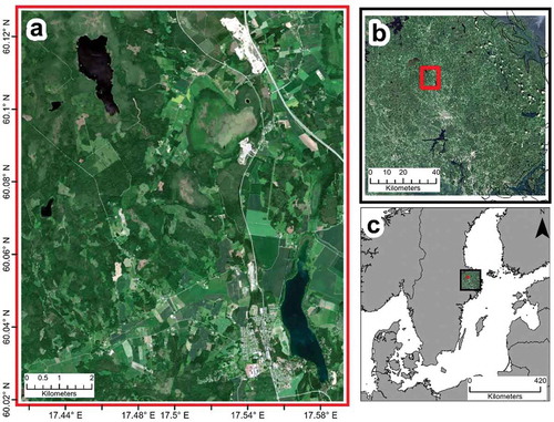
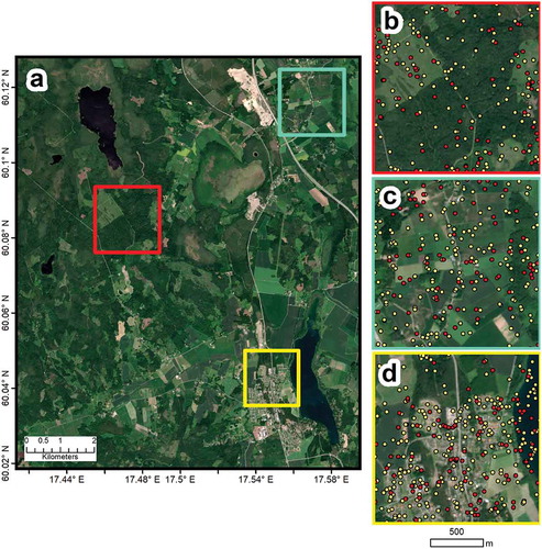
The study area (Figure 1) is a 10 km x 12 km mixed-use landscape located in the county of Uppsala in south-central Sweden. The mean annual temperature and precipitation are 5.6°C and 597 mm, respectively (Fick and Hijmans 2017). The elevation of the area is 40 meters above mean sea level (Tachikawa et al. 2011) and comprises stands of Norway spruce (Picea abies), Scots pine (Pinus sylvestris), and birch (Betula sp.), as well as extensive agriculture (Lundin et al. 1999). This area was specifically selected because of the weak annual amplitude of the vegetation greenness, which makes it difficult to capture seasonality (Jönsson et al. 2018) and thus poses a classification challenge, particularly for differentiation between vegetation types. The area also includes the Norunda research site that was established in 1994 for studies of greenhouse gas exchange, energy and water using the eddy covariance method. The research site is presently managed by Lund University and forms part of the Swedish contribution to the European research infrastructure Integrated Carbon Observation System.

Figure 1. a) Study area; b) location of the study area within the 33VXG Sentinel-2 tile; c) overview of the 33VXG tile’s coverage relative to Sweden and the Baltic region.

3. Data

3.1. Sentinel-2 data

The Sentinel-2 Multispectral Instrument (MSI) comprises two satellites that observe the Earth at 10 m, 20 m, and 60 m spatial resolutions (Drusch et al. 2012). The 10 m spatial resolution is the highest amongst freely available satellite products. Another unique aspect of the Sentinel-2 data is the presence of three red edge bands, which are able to capture the strong reflectance of vegetation in the near infrared portion of the electromagnetic spectrum (EMS).

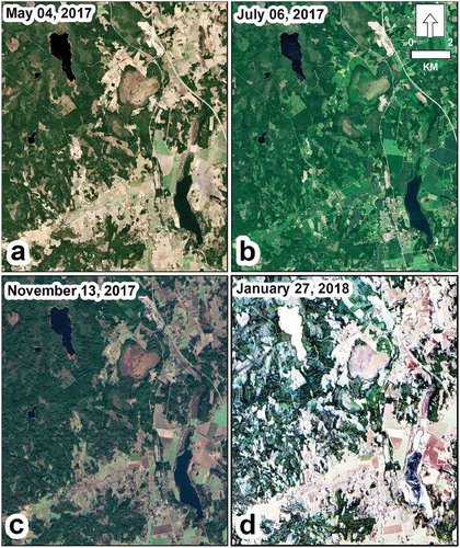
The criteria for satellite imagery selection was that the scenes must contain little or no clouds and haze. The imagery must also be from different seasons to capture different plant phenological stages. As such, four Sentinel-2 scenes from 2017 and 2018 from tile 33VXG were included in the analysis. Three of the scenes were in 2017: May 04, July 06, and November 13, and one in 2018: January 27 (Figure 2). All the images were captured by Sentinel-2A except for the 2018 image, which was from Sentinel-2B. As shown in Table 1, the twin Sentinel satellites do not have identical band structures and the mean difference in the central wavelength of the ten bands used in this study is 3.3 ± 4.6 nm. The satellite imagery was downloaded from the Copernicus Open Access Hub (https://scihub.copernicus.eu/) on 29 May 2018. These were in Level-1C processing format, which means that they underwent geometric and radiometric correction but were not atmospherically corrected (Drusch et al. 2012). Atmospheric correction was performed using Sen2Cor (v2.5.5), which converts the top-of-atmosphere reflectance Level-1C data to a bottom-of-atmosphere (BOA) reflectance Level-2A product (Müller-Wilm 2018). BOA is also called “surface reflectance,” i.e. reflectance that would be measured at land surface, and is hereafter referred to as such. Ten bands that cover the red, blue, green, red edge, near- and short-wave infrared portions of the EMS were selected for inclusion into the classification procedure (Table 1). All the bands at 20 m spatial resolution were resampled to 10 m using bilinear interpolation to facilitate integration and consistency.

Table 1. Descriptions of the 10 Sentinel-2 bands used in this study. SR = Spatial Resolution, CW = Central Wavelength.

			S2A		S2B
Band	Spectral Region	SR(m)	CW(nm)	Bandwidth (nm)	CW(nm)	Bandwidth (nm)	CW Difference
2	Blue	10	496.6	98	492.1	98	4.5
3	Green	10	560.0	45	559	46	1
4	Red	10	664.5	38	665	39	0.5
8	Near Infrared	10	835.1	145	833	133	2.1
5	Red Edge	20*	703.9	19	703.8	20	0.1
6	Red Edge	20*	740.2	18	739.1	18	1.1
7	Red Edge	20*	782.5	28	779.7	28	2.8
8A	Near Infrared	20*	864.8	33	864	32	0.8
11	Shortwave Infrared	20*	1613.7	143	1610.4	141	3.3
12	Shortwave Infrared	20*	2202.4	242	2185.7	238	16.7

*Resampled to 10 m.

Figure 2. Natural color composites of the multi-temporal imagery used in this study. a) 4 May 2017 (Sentinel-2A); b) 6 July 2017 (Sentinel-2A); c) 13 November 2017 (Sentinel-2A); d) 27 January 2018 (Sentinel-2B).

Three spectral indices were derived from the resultant bands of each Sentinel-2 scene. The normalized difference vegetation index (NDVI) quantifies the ratio between energy absorbed by the vegetation canopy in the red portion of EMS and the energy reflected in the near infrared (NIR) (Rouse et al. 1973). The modified normalized difference water index (MNDWI) is a ratio index that maximizes the reflectance of water by using the green portion of the EMS while using the shortwave infrared (SWIR) portion to suppress the influence from artificial surfaces (Xu 2006). The normalized difference built-up index (NDBI) uses the SWIR band to identify artificial surfaces because of their strong reflectivity in that portion of the EMS while using the NIR to suppress the influence of vegetated surfaces (Zha, Gao, and Ni 2003). NDVI, MNDWI, and NDBI were included in the classification process in order help capture vegetation, water, and artificial surfaces, respectively. This resulted in each Sentinel-2 scene having 13 layers (10 bands + 3 indices) for a total of 52 layers.

4. Methods

4.1. Study design and sample selection

Training data are crucial components in supervised learning and most machine learning algorithms require a large number of training data samples. However, the delineation and acquisition of reference data from satellite imagery can be a daunting task (Chi, Feng, and Bruzzone 2008). In-situ collection of representative training data is difficult over large, remote or distant areas (Inglada et al. 2017) and the use of timely high-resolution satellite or aerial imagery for this purpose is not always feasible and often cost-prohibitive. The use of old maps as ancillary data for classifying past land-cover is not an uncommon practice in the remote sensing community. For example, Tran, Tran, and Kervyn (2015) used thematic maps from the 1970s as training input to classify Landsat-1 data from 1973 over a study area in Vietnam. A novel approach being applied in a growing number of recent studies is that training data are acquired from extant high-quality land-cover maps (Wessels et al. 2016; Zhang and Roy 2017; Hermosilla et al. 2018). The use of an existing maps as training data for LCLU classification can introduce errors inherent in the previous classification. However, land-cover maps with reasonably high overall accuracy can produce a large number of training samples with increased efficiency allowing for a wide range of feature representation (Hermosilla et al. 2018). Further, it is important to randomly check the accuracy of the training samples collected from these land-cover maps in order to minimize misclassification, for example, to ensure that a sample labeled as “forest” actually falls within a forest.

The study design (Figure 3) involves initial training sample selection with orthophotos then increasing the sample size using a high-quality LCLU map of the study area. A total of 100 training samples were initially collected for each land-cover class in the study area using random sampling from 25 cm orthophotos of the study area captured on the 2^nd and 3^rd of July 2015 by the Swedish Cadastral and Land Registration Authority (https://zeus.slu.se). These samples were then compared to RGB and false color composites of the multi-temporal Sentinel-2 scenes to discern any visible change that took place between 2015 and 2017/18 such as clearcutting or infrastructure development. The sample labels were modified in the event that a change was detected. In the next step, each of the samples was compared to the 2018 National Land Cover Database of Sweden (Nationella marktäckedata, NMD), produced by the Swedish Environmental Protection Agency with a minimum mapping unit of 0.01 hectares. Again, sample labels were modified where appropriate as described in the next paragraph. The NMD dataset was the result of an integrated processing chain that involves several ancillary datasets from Swedish Cadastral and Land Registration Authority (Lantmäteriet), Statistics Sweden (Statistiska centralbyrån), road and railway network data, 25 cm orthophotos, a 2 m digital elevation model, and airborne lidar. The NMD is part of Sweden’s national geo-strategy for 2016–2020 and is available from https://www.naturvardsverket.se/.

Figure 3. Flowchart of the methods.

Fifteen of the 25 NMD classes occurred in the study area and were aggregated to eight classes (Table 2). These are: (1) Deciduous forest: comprising birch, aspen, alder, beech, oak, elm and ash; (2) Coniferous forest: comprising Scots pine and Norway spruce; (3) Water: lakes, rivers and canals; (4) Artificial: urban areas, construction sites, and roads; (5) Wetlands: saturated land including marshes and bogs; (6) Agriculture; (7) Clear cuts within and outside wetlands; and (8) Open land with and without vegetation. The remaining seven classes were discarded due to negligible presence in the study area. A quantitative sample-by-sample inspection resulted in a low (1.75%) mismatch between the NMD dataset and the 800 samples (100 samples per class) collected using the orthophotos, and a qualitative visual inspection showed a good match between the NMD classes and the orthophotos (Figure 4). In this way, the reference data can reliably replicate on-ground conditions and meet the good practice guidance for accuracy assessment (Olofsson et al. 2014).

Table 2. Total number of pixels in each sample and the number of pixels selected for the training and evaluation. The sum of training and evaluation pixels represents 1% of all pixels in the study area. Also shown are the original Swedish National Land Cover Database (NMD) classes that were aggregated to form each of the eight land cover types in this study. Forest classes are all outside of wetlands.

LCLU Type	Class ID	Original NMD Class Description	Pixels (Total)	Samples (Training/Evaluation)
Deciduous	Class 1	1.1.5 Birch, Aspen, and Alder forest	180,827	8271/3544
		1.1.6 Beech, Oak, Elm, and Ash forest
Coniferous	Class 2	1.1.1 Scots pine forest	411,356	8271/3544
		1.1.2 Norway spruce forest
		1.1.3 Mixed coniferous forest
Water	Class 3	6.1 Water	45,222	8271/3544
Artificial	Class 4	5.1 Developed land, building	52,839	8271/3544
		5.2 Developed land, no building/road
		5.3 Developed land, road
Wetland	Class 5	2 Wetland	44,835	8271/3544
Agriculture	Class 6	3 Agriculture	261,391	8271/3544
Clear Cut	Class 7	1.1.8 Clear cut outside wetlands	125,476	8271/3544
		1.2.8 Clear cut within wetlands
Open Land	Class 8	4.1 Open land without vegetation	56,497	8271/3544
		4.2 Open land with vegetation

Next, the number of samples was increased using the NMD dataset due to the data-driven framework of machine learning models (Brink, Richards, and Fetherolf 2017). Stratified random sampling was applied in order to produce 1477 samples per class. This number was selected because it represents 1% of all the pixels in the study area when all the class samples are summed (1477 x 8 = 11,816). This amount of samples was chosen because it is large enough to be adequately dispersed across the study area (Figure 5) and does not exhaust available computing power. The 11,816 samples were then split into two portions: a training dataset comprising 70% (8271) of the samples and an evaluation dataset comprising the remaining 30% (3544). Each LCLU class was assigned the same number of training (1034) and evaluation (443) samples (Table 2).

Figure 4. Comparison between the 25 cm orthophotos from 2015 (a-labeled panels) and the 2018 Swedish National Land Cover Database (NMD) map (b-labeled panels) for different parts of the study area.

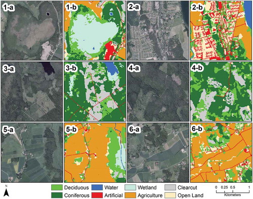
Figure 5. Overview of the training (yellow dots) and evaluation (red dots) samples in selected parts of the study area: (a) The full study area; (b) red box: within the vicinity of the Norunda research station; (c) turquoise box: agricultural fields of Örbyhus in the northeast of the study area; (d) yellow box: the town of Björklinge in the southeast..

4.2. Machine learning algorithms

This section provides descriptions of the algorithms used in the classification. Readers seeking deeper understanding of the theoretical background of a particular algorithm should consult the reference provided at the end of each description.

4.2.1. Support vector machines

SVM was first described in Cortes and Vapnik (1995) based on the work of Vapnik (1982) and is a supervised learning technique commonly used in a range of remote sensing applications. The SVM algorithm finds the optimum minimization, i.e. decision boundary, of ambiguous classifier outputs in a problem space. This decision boundary is referred to as the hyperplane and it distinguishes the classification problem into a predefined set of classes that are consistent with the training data. The algorithm undergoes an iterative process of finding the optimum hyperplane boundary in an n-dimensional classification space to distinguish patterns in the training data then apply the same configuration to a separate evaluation dataset. The dimensions in this context are the number of spectral bands and the vectors are the individual pixels in a multiband composite (Mountrakis, Jungho, and Ogole 2011). There are different kernels through which the hyperplane boundary can be defined. Here, a radial basis function kernel was used because some of the Sentinel-2 bands are not linearly separable. A detailed mathematical description of this algorithm can be found in Cortes and Vapnik (1995).

4.2.2. Random forests

RF is an ensemble learning algorithm based on the idea that a combination of bootstrap aggregated classifiers perform better than a single classifier (Breiman 2001). The bootstrap component means that each individual tree is parameterized using a randomly sampled set of observations with replacement from the training data (Hastie, Tibshirani, and Friedman 2009). This helps to de-correlate the trees thereby reducing multicollinearity. The proportion of observations that are not used for this purpose are included in the evaluation and are referred to “out-of-bag” samples. Several of these decision tree models are created on different groupings of the input variables and the resultant output is the unweighted majority vote of each class that is averaged across all trees. A detailed mathematical description of RF is provided in Breiman (2001).

4.2.3. Extreme gradient boosting

The classical gradient boosting machine (GBM) builds an additive model of shallow decision trees that are weak learners and then generalizes them by optimizing an arbitrarily defined loss function to make stronger predictions (Friedman 2001). Xgboost is a relatively new implementation of the GBM that simultaneously optimizes the loss function while building the additive model (Chen and Guestrin 2016). The novelty of Xgboost lies in the fact that it comprises an objective function, which combines the loss function and a regularization term that controls model complexity. This enables parallel calculations and the maintenance of optimal computational speed. The softmax multiclass classification objective function was used in this study. Softmax is a function that normalizes each class into a probability distribution with an interval of (0, 1) that sums to 1. A detailed mathematical description of Xgboost is provided in Chen and Guestrin (2016).

4.2.4. Deep learning

The type of DL architecture implemented in this study is a multilayered feed-forward deep neural network (DNN) with error back-propagation. DNN links several functions joined together in hierarchically structured neural networks that are typically deeper than three hidden layers. The information flows from the input data through the activation function, error is calculated and propagated back to the earlier layers, and finally fed to the output at the conclusion of the predefined iteration (Candel and Erin 2018; Goodfellow, Bengio, and Courville 2016). In this way, every sequential hidden layer merges values in the previous layer and subsequently learns to form more abstract representations until the output layer. The algorithm exploits the activation function by learning the values of parameters that result in the best approximation (Beysolow 2017). These are then taken by an output function that computes class probabilities. The hyperbolic tangent (tanh) activation function with a softmax output classification function were used in this study. Tanh is a rescaled logistic sigmoid function, i.e. $f(x)={\left(1+e^{-x}\right)}^{-1}$, that provides zero-centered outputs and allows model parameters to be more frequently updated in feed-forward neural networks. A detailed description of the DL method applied in this study is provided in Goodfellow, Bengio, and Courville (2016) and in Candel and Erin (2018).

4.3. Model training and hyper-parameter optimization

Hyper-parameter optimization (also called tuning) was part of the model training process whereby optimal hyper-parameters were selected for the algorithms. Models were trained by optimizing hyper-parameters using a repeated k-fold cross-validation. In the case of SVM, RF and Xgboost, optimization was performed using randomized sampling of all hyper-parameter combinations up to a specified number of iterations (Kuhn and Johnson 2013b; Bergstra and Bengio 2012). This is called the tune length and it defined the total number permutations that were evaluated. The training dataset was randomly split into k sets of equal size, of which one set was retained for validation and the remaining k–1 samples were used for training. The entire procedure was then repeated using a predefined set of repeats in order to reduce model variance (Kim 2009; Kuhn and Johnson 2013a). A 10-fold cross-validation with 5 repeats was chosen as a tradeoff between lowering the variance, ensuring a robust model, and a reasonable computational time.

In case of DL, optimization was performed using a random grid search. Here, the algorithm trained a model for all possible combinations of the hyper-parameters in the grid and selected the best one. Once the tune length was reached, the performance metrics from the cross-validation were used to select the best model parameters (Table 3). SVM, RF, and Xgboost were run using the caret package (Kuhn 2008) in the R statistical software environment version 3.4.2 (R Core Team 2017). DL was performed using the H2O package, also in R (Cook 2016). All processing was performed on an 8-core 3.60 GHz Xeon server with 48 GB of RAM running Windows 10 64-bit.

Table 3. Results of the hyper-parameter optimization process showing the final values used in each model. The tune length was set to 1000 iterations. SVM = Support Vector Machines, RF = Random Forest, XGB = Extreme Gradient Boosting, DL = Deep Learning. Algorithms were run in R using the caret package (Kuhn 2008) and the H2O package (Cook 2016).

Model	Hyper-parameter Value	Definition
SVM	sigma = 0.00425, C = 64, Kernel = “rbf”	rbf = radial basis function, a multidimensional Gaussian distribution function describing the distance between an input vector and a pre-defined center vector. sigma = weight of the RBF kernel. C = cost of misclassification.
RF	mtry = 7, ntree = 1000	mtry = number of variables randomly sampled as candidates at each split. ntree = number of trees.
XGB	nrounds = 500 max_depth = 10 eta = 0.05 gamma = 0.3 nodesize = 1	nrounds = maximum number of iterations. max_depth = maximum depth of a tree. eta = learning rate by which to shrink the feature weights. gamma = minimum relative improvement in squared error reduction in order for a split to happen. nodesize = minimum number of rows to assign to the terminal nodes.
DL	activation = “tanh,” hidden_layers = 6, neurons_per_layer = 200, epochs = 500	activation = activation function. hidden_layers = number of hidden layers. neurons_per_layer = size of each hidden layer. epochs = number of times to iterate.

4.4. Accuracy assessment and area estimation

The accuracy of each algorithm was assessed using a number of metrics derived from an error matrix. These include Overall Accuracy (OA), Producer’s Accuracy (PA), and User’s Accuracy (UA). Error matrices were enhanced by providing unbiased estimations of the proportional area of cells within the matrix as per Olofsson et al. (2014). The area proportions of the mapped classes were included in the output because each class required its own estimation weight. These proportions were necessary to estimate OA and PA in order to include differences in sampling between classes. Conversely, UA was computed from within a given LCLU class and was thus retrieved directly from the error matrix (Olofsson et al. 2013).

McNemar’s chi-squared (χ²) test (McNemar 1947) was used to statistically compare error matrices by testing for the marginal homogeneity between two classifiers. Marginal homogeneity refers to the equality (i.e. lack of statistically significant difference) in the overall distributions of row or column variables predicted by one algorithm compared to another. It is a simple yet powerful method to compare class-wise predictions between algorithms. The test is parametric, has a low type I error and consists of a straightforward formulation (Dietterich 1998; de Leeuw et al. 2006). Additionally, a two-proportion Z-test (Lachin 1981) was used to compare the proportions of correctly classified pixels (PCCP) from two algorithms at a time. This test produced a two-tailed probability value that tests the null hypothesis of no difference between PCCP of each algorithm pair. The square of the Z-statistic produced by the test followed a χ² distribution with one degree of freedom (Wallis 2013). For both methods, a χ² value of greater than 3.84 indicated statistically significant difference at the 5% level.

The conventional method of computing areas of mapped classes involves multiplying the area of a pixel by the total number of pixels in a class. This method does not account for classification errors (Czaplewski 1992) and introduces bias into the resultant LCLU map. Therefore, in order to provide unbiased area estimates of the output classes, error-adjusted stratified estimation of the error matrix was conducted following Olofsson et al. (2013). Each area estimate was accompanied by a confidence interval (95%) that quantified uncertainty. For a thorough explanation of the method used to acquire these unbiased accuracies and quantify uncertainty in area estimates, readers are strongly encouraged to consult the good practices guide by Olofsson et al. (2014) and the recommendations described in Olofsson et al. (2013).

5. Results and discussion

5.1. Classifier comparison

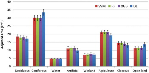
The OA of the four algorithms were relatively close to one another as shown in Table 4. These accuracies were derived from the error matrix shown in Figure 6. The highest OA was produced by SVM (0.758 ± 0.017), closely followed by Xgboost (0.751 ± 0.017) and RF (0.739 ± 0.018), and finally DL (0.733 ± 0.0023). All four algorithms produced similar maps that were visually appealing (i.e. coherent classes and minimal speckling) and represented the area fairly well (Figure 7). The adjusted areas of the classes within a 95% confidence interval were similar for SVM, Xgboost and RF. However, relative to the other algorithms, DL overestimated coniferous forests and open land, and underestimated the remaining classes except water (Figure 8). All eight LCLU classes had the same number of training and evaluation samples so that the OA is not biased towards classes with more training samples (He and Garcia 2008). One drawback of balanced training samples in conventional accuracy assessment is that the proportions of land-cover classes are not taken into consideration. However, area proportions were taken into account in this study using by producing unbiased OA estimates following Olofsson et al. (2014), which could have led to lower OA. It is possible to obtain higher OA values using an imbalanced class distribution where the accuracy of certain well-represented classes increases OA. But, this focus on OA ignores the performance of individual classes and is particularly disadvantageous to those that are underrepresented in the study area (Maxwell, Warner, and Fang 2018). Therefore, the choice of sampling design should be dependent upon whether the objective of the study is to obtain the highest possible OA regardless of class distribution or equally represent all LCLU classes.

Table 4. Area-adjusted performance metrics for each machine learning algorithm and LCLU class derived from the error matrices in Figure 6. The proportional weights of each class that were used to create the unbiased error estimate for each class. SVM = Support Vector Machines, RF = Random Forest, XGB = Extreme Gradient Boosting, DL = Deep Learning, OA = Overall Accuracy.

		Producer’s Accuracy	User’s Accuracy	Class Weight	Area in km^2	Number of Pixels
SVM OA = 0.758 ± 0.017	Deciduous	0.63	0.69	0.1412	17	166,886
	Coniferous	0.94	0.74	0.3216	38	380,212
	Water	0.93	0.99	0.0381	5	45,047
	Artificial	0.45	0.72	0.0589	7	69,645
	Wetland	0.69	0.90	0.0466	6	55,134
	Agriculture	0.93	0.85	0.1938	23	229,077
	Clear cut	0.73	0.71	0.1280	15	151,311
	Open land	0.49	0.64	0.0718	8	84,900
RF OA = 0.739 ± 0.018	Deciduous	0.63	0.64	0.1461	17	172,733
	Coniferous	0.93	0.74	0.3163	37	373,906
	Water	0.92	0.98	0.0381	5	45,090
	Artificial	0.40	0.72	0.0535	6	63,212
	Wetland	0.67	0.85	0.0486	6	57,419
	Agriculture	0.93	0.86	0.1954	23	230,974
	Clear cut	0.67	0.65	0.1256	15	148,453
	Open land	0.47	0.59	0.0765	9	90,425
XGB OA = 0.751 ± 0.017	Deciduous	0.64	0.68	0.1427	17	168,754
	Coniferous	0.94	0.75	0.3175	38	375,365
	Water	0.93	0.98	0.0388	5	45,872
	Artificial	0.45	0.72	0.0586	7	69,301
	Wetland	0.65	0.89	0.0470	6	55,573
	Agriculture	0.93	0.85	0.1957	23	231,346
	Clear cut	0.70	0.67	0.1247	15	147,476
	Open land	0.46	0.59	0.0749	9	88,525
DL OA = 0.733 ± 0.0023	Deciduous	0.58	0.63	0.1334	16	157,741
	Coniferous	0.95	0.75	0.3548	42	419,436
	Water	0.93	0.98	0.0384	5	45,381
	Artificial	0.36	0.71	0.0424	5	50,078
	Wetland	0.64	0.88	0.0451	5	53,309
	Agriculture	0.90	0.78	0.1884	22	222,755
	Clear cut	0.70	0.66	0.1173	14	138,674
	Open land	0.44	0.64	0.0802	9	94,838

Figure 6. Error matrices showing correct and incorrect cross-tabulations of the evaluation samples by each machine learning algorithm. The LCLU classes are numbered 1 through 8, where 1 = Deciduous, 2 = Coniferous, 3 = Water, 4 = Artificial, 5 = Wetland, 6 = Agriculture, 7 = Clear cut, 8 = Open land. The error matrices form the basis for the calculation of the performance metrics shown in Table 4.

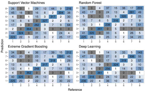
Figure 7. Final classified maps of the study area for (a) Support Vector Machines; (b) Random Forests; (c) Extreme Gradient Boosting; (d) Deep Learning.

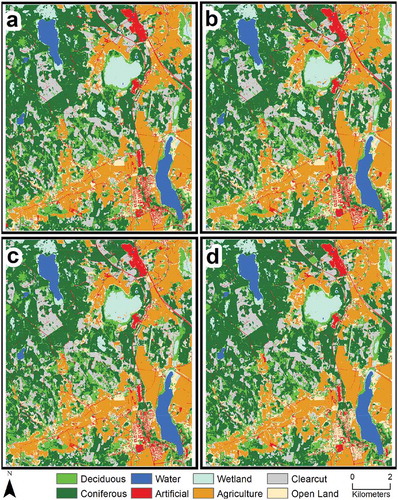
Figure 8. Adjusted area estimates of each LCLU class resulting from image classification using the four algorithms tested. The error bars denote the 95% confidence interval. SVM = Support Vector Machines, RF = Random Forest, XGB = Extreme Gradient Boosting, DL = Deep Learning.

The lowest PA across all four algorithms was for open land and artificial surfaces (Table 4), which highlights the difficulty distinguishing these classes from the rest. Open land was composed primarily of grasses and herbs, and was visually similar to clear cuts, particularly those with regrown shrubs and herbaceous cover. Thus, it remained difficult to classify due to the similar spectral properties of the vegetation found in it (Buck et al. 2015). On the other hand, artificial surfaces in the study area consisted of suburban features such as small towns and villages interspersed with vegetation such as trees and grass. The inclusion of land surface temperature (Abdi 2019) could have enhanced the detection of man-made features but there is presently no straightforward way to quantify emissivity because the MSI lacks a thermal band.

SVM produced the highest accuracy for open land (PA = 0.49) among the four classifiers, and tied with Xgboost for artificial surfaces (PA = 0.45). The ability of SVM to capture these classes was probably because it is based on a relatively small number of complex decision boundaries (Cortes and Vapnik 1995). In cases such as open land and clear cuts, where the data were linearly non-separable, the feature vectors were projected with a nonlinear vector mapping function to a higher dimension feature space. This facilitates the creation of a decision boundary that seems nonlinear in the original feature space. The added computation intensity of this projection was offset, to a certain extent, by kernel functions that enable a simplified representation of the data (Mountrakis, Jungho, and Ogole 2011). Indeed, Khatami, Mountrakis, and Stehman (2016) found that SVM was the most efficient algorithm for most applications and outperformed several classifier families, including RF, neural networks, and decision trees in direct comparison.

A somewhat surprising result was that DL produced the lowest accuracy for open land and for artificial surfaces (PA = 0.44 and 0.36, respectively), and was overall the poorest performing algorithm. Use of the tanh activation function was the probable reason for the underperformance of DL in this study. The tanh function easily saturates (i.e. the so-called “vanishing gradient problem”) and slows the training procedure when applied to DNNs (Rakitianskaia and Engelbrecht 2015). In the case of high-dimensional data such as multi-temporal satellite imagery, this saturation was possibly dependent on feature complexity. The tanh activation function has a conventional sigmoid curve that is centered at zero and is restricted to the range of (−1, 1). It returns a near-zero slope when the input values are large (Shi et al. 2018). This suggests that it was incapable of the separating the complex multiclass features in the study area. The DL classes with the highest PA were those that can be relatively easily distinguished from multi-temporal data such as coniferous forests, water or agriculture (Table 4). The lowest performing DL classes are spectrally complex and thus had considerable variation in the relative intensity of pixel reflectance and the tanh activation function performed poorly in distinguishing between them. In retrospect, the rectified linear units (ReLU) activation function may have provided a better output due to its ability to hold the incremental gradient descent, i.e.$f(x)=max\left[0,x\right]$, because it is a non-saturating nonlinearity function (Nair and Hinton 2010).

McNemar’s test results (Table 5) showed that 42% of the class-wise predictions between paired algorithms exhibited significance at the 1% level (P ≤ 0.01); 20% at the 5% level (P ≤ 0.05); and 11% at the 10% level (P ≤ 0.10). Additionally, 27% of class-wise algorithm pairings were statistically non-significant. Most of the non-significant pairings were for wetland, except between Xgboost and SVM (P ≤ 0.05) and between Xgboost and DL (P ≤ 0.10). This means that apart from these two pairings, accuracies for wetland between the other classifiers were statistically insignificant, i.e. there is no real difference between them. Both coniferous forests and clear cuts were consistent at the 1% level across all classifier pairings, suggesting that the accuracies achieved for these classes were highly significant.

Table 5. McNemar’s chi-squared (χ²) test with associated probability value (P). SVM = Support Vector Machines, RF = Random Forest, XGB = Extreme Gradient Boosting, DL = Deep Learning. *** = P ≤ 0.01, ** = P ≤ 0.05, * = P ≤ 0.1, NS = Not Significant.

	McNemar’s Test	Deciduous	Coniferous	Water	Artificial	Wetland	Agriculture	Clear Cut	Open Land
SVM v. RF	χ^2	11.589	42.654	3.184	6.298	0.985	0.041	27.876	7.557
	P	***	***	*	**	NS	NS	***	***
XGB v. SVM	χ^2	18.178	45.797	2.132	3.838	4.621	0.071	31.045	4.951
	P	***	***	NS	**	**	NS	***	**
DL v. SVM	χ^2	5.320	36.445	3.184	1.098	1.071	3.923	52.115	59.602
	P	**	***	*	NS	NS	**	***	***
RF v. XGB	χ^2	8.983	41.150	1.841	12.445	2.756	0.018	28.019	3.71
	P	**	***	NS	***	NS	NS	***	**
DL v. RF	χ^2	1.227	32.345	2.750	6.892	0.386	4.498	47.036	52.998
	P	NS	***	NS	***	NS	**	***	***
XGB v. DL	χ^2	3.432	35.003	1.841	4.331	2.984	4.188	51.336	46.066
	P	*	***	NS	*	*	**	***	***

The Z-test results (Table 6) showed that the PCCP of two algorithm pairings were statistically significant thereby rejecting the null hypothesis. These are SVM and RF (χ² = 4.832), and SVM and DL (χ² = 4.701). This indicates that the PCCP produced by SVM is markedly different from those produced by RF and DL despite the fact their OA are fairly close to one another (Table 4). For the remaining four algorithm pairings, the null hypothesis was not rejected, meaning their accuracies are similar. Although the PCCP produced by SVM and Xgboost are not statistically different from one another (χ² = 1.369), the latter failed to reject the null hypothesis when compared to other algorithms (Table 6).

Table 6. A Two Proportion Z-test to compare the proportions of correctly classified pixels with its associated probability value (P). SVM = Support Vector Machines, RF = Random Forest, XGB = Extreme Gradient Boosting, DL = Deep Learning. Algorithm pairs that exhibit a statistically significant (P ≤ 0.05) difference in the proportion of correctly classified pixels are in bold.

Algorithm Pair	Two Proportion Z-test
SVM v. RF	χ^2 = 4.832
	P = 0.027
XGB v. SVM	χ^2 = 1.369
	P = 0.241
SVM v. DL	χ^2 = 4.701
	P = 0.030
RF v. XGB	χ^2 = 0.996
	P = 0.318
DL v. RF	χ^2 = 0
	P = 1
XGB v. DL	χ^2 = 0.937
	P = 0.333

A possible limitation of the classification process was the choice of user-defined parameters for each algorithm (Table 3). The hyper-parameter optimization applied here was based on iterative tuning and a random grid search without empirically examining their optimum values. This was done in order to compare the algorithms in a fair manner and not introduce a priori knowledge. Thus, the accuracies reported here may not represent the maximum possible that could be attained. That said, the removal of open land, which was one of the confusion classes, increased the overall accuracy for all algorithms by an average of 15% with Xgboost having 0.7% higher accuracy than SVM (not shown). A complex landscape invariably includes classes that are spectrally similar to one another, such as open land and clear cuts in this study, but that have different land-use categorizations. Therefore, an algorithm’s ability to generalize training samples within such classes will ultimately be reduced. This leads to a non-separation of these classes in a feature space causing overlap between class distributions and a lower overall classification accuracy (Jansen and Gregorio 2002; Smits, Dellepiane, and Schowengerdt 1999).

5.2. Variable importance metrics

All four algorithms provide variable importance metrics as part of their output (Supplementary Figure 1–4). The twenty highest scoring layers across the three algorithms displayed two generalizable patterns of importance. First, nearly half belonged to the red edge (25%) and shortwave infrared (SWIR) (23%) bands. Second, they were dominated by scenes from May (38%) and July (40%). None of the spectral indices were ranked highly in this study. In the case of NDVI, it was probably due to the red edge bands providing most, if not all, of the information required to account for the vegetation signal. Additionally, NDVI is known to saturate at high values (Box, Holben, and Kalb 1989), which further degrades its ability to capture high-biomass classes such as forests. The absence of the other two indices could be explained by inability to separate urban areas and barren land in the case of NDBI (Zha, Gao, and Ni 2003), and between water and shadowed surfaces in the case of MNDWI (Feyisa et al. 2014).

A distinguishing feature of the Sentinel-2 satellites is the presence of red edge bands that provide an added value previously only available in commercial satellites such as RapidEye. The red edge region is so-called because leaves reflect strongly between 680 nm and 780 nm and is dependent on chlorophyll concentration (Horler, Dockray, and Barber 1983; Gates et al. 1965). The advantage of the red edge bands in LCLU classification is evident when Sentinel-2 data is compared with other satellites such as Landsat-8 that do not capture this portion of the EMS. For example, red edge Band 5 (705 nm) was found to be important for mapping crop types, particularly cereals and legumes (Forkuor et al. 2018), red edge Band 6 (740 nm) was useful for differentiating crop types from grassland at the sub-pixel level (Radoux et al. 2016), and red edge band 7 (783 nm) was used for classifying edge pixels in boreal forests comprising Scots pine, Norway spruce and birch (Zerega 2018).

The high importance of the SWIR bands could be due to the dominance of forest classes in the study area (Eklundh, Harrie, and Kuusk 2001). Sentinel-2’s SWIR bands are centered at 1610 nm (Band 11) and 2190 nm (Band 12) and were thus able to detect variability in water content between different tree species (Lukeš et al. 2013). The combination of red edge bands with SWIR has been shown to enhance the modeling of boreal forest canopy cover and leaf area index, producing root-mean-square error values 1.6–7.2% lower than Landsat-8 (Korhonen, Hadi, and Rautiainen 2017). Sentinel-2 Band 11 was also found to correlate well (r = −0.68, p = 0.01) with Mediterranean forest growing stock volume (Chrysafis et al. 2017), although in a Swedish forest Zerega (2018) found a lower correlation for Band 11 (r = −0.26) and higher correlations (−0.51 and −0.52) for red edge bands 6 and 7, respectively. Recent work by Persson, Lindberg, and Reese (2018) to classify Norway spruce, Scots pine, hybrid larch, birch and pedunculate oak found that red edge bands captured in May and July and SWIR bands captured in April and October had the highest separation of the tree species.

A possible limitation of the variable selection process was the fact that different algorithms calculate variable importance differently. For example, the DL implementation in H2O used a method by Gedeon (1997) that accounts for each input variable’s connecting weights to the first two input layers as a basis for computing its importance. Both RF and Xgboost computed variable importance in similar ways that were based on the mean decrease of a predefined loss function such as mean squared error (Breiman 2001; Chen and Guestrin 2016). Despite these differences, the results (Supplementary Figure 1–4) illustrate the consistency with which red edge and SWIR bands from May and July were selected by the algorithms.

5.3. Mono-temporal vs. multi-temporal Sentinel-2 data

The rationale for incorporating data from four seasons was to help distinguish vegetation classes that had different phenological cycles (e.g. coniferous, deciduous, crops). However, the importance of the scenes from May and July was clear in this study, which was probably due to the dominance of forest area (Figure 8), and the increased leaf expansion in the boreal zone that usually takes place in late spring – early summer (Tang et al. 2016). Increase in the light-saturated mean daily rate of photosynthesis also takes place around that time as the seasonal light intensity increases with the approaching boreal summer (Sukenik, Bennett, and Falkowski 1987; Letts et al. 2008). Canopy maturation takes place around July, which is also an important time for the maturation of certain crops, such as wheat, that require relatively dry sunny conditions (Brown 2013; Tang et al. 2016).

The use of multi-temporal data may have inadvertently increased the level of noise in the classification process as increased data dimensionality leads to higher redundancy (Nitze, Barrett, and Cawkwell 2015). Indeed, bootstrapped accuracy provided by RF showed a steep decline with the addition of new variables after reaching peak accuracy with just six bands. This may suggest that mono-temporal (i.e. a single scene) Sentinel-2 surface reflectance data, captured within an optimal date (Vuolo et al. 2018), may offer an alternative to multi-temporal time series. This could be due to the relatively high radiometric resolution of Sentinel-2 data, particularly the presence of three red edge and two near infrared bands that enable the satellites to sense important biophysical parameters. Furthermore, differences in radiometry between Sentinel-2A and Sentinel-2B were unlikely to have impacted the results as the mean difference in the central wavelength of the bands used was 3.3 ± 4.6 nm and there was considerable overlap between the bandwidths of the two satellites (Table 1).

Early work on Sentinel-2 data by Immitzer, Vuolo, and Atzberger (2016) found that mono-temporal Sentinel-2 red edge and SWIR were important for mapping both tree species and crop types. However, the timing of the imagery used (13 August for trees and 30 August for crops) caused confusion within these classes. The dates of these acquisitions were not optimal because most crops were approaching senescence while images acquired at the end of spring would have better differentiated tree species (Immitzer, Vuolo, and Atzberger 2016; Persson, Lindberg, and Reese 2018). The authors thus concluded that they expect multi-seasonal information contained within time-series of Sentinel-2 data to provide improved classification results. Persson, Lindberg, and Reese (2018) used Sentinel-2 images from four months (April, May, July and October) in 2017 to classify tree species in Sweden. They found that although the highest OA of 88.2% was obtained when all bands from all four dates were included, the highest accuracy provided by a single image (80.5%) was the one from May.

It is not implausible that a single, optimally-timed, atmospherically-corrected Sentinel-2 scene could provide equal or better results than a multi-temporal stack for detecting spectral differences in vegetation due to the accumulation of noise that is inherent in such data (Feilhauer et al. 2013). Of course, this is highly dependent on the aims that a study hopes to achieve. For example, Prishchepov et al. (2012) found that in order to map land abandonment with classification accuracies greater than 80%, it was necessary to use at least three multi-temporal images within a single year before and after abandonment. Phenological information contained within multi-temporal data does allow for better discrimination between spectrally similar and phenologically distinct vegetation. However, it should be used with caution in managed land due to anthropogenic changes that could be confused for phenological change (Ghioca-Robrecht, Johnston, and Tulbure 2008).

6. Conclusions and recommendations

The Sentinel-2 Multispectral Instrument is unique among presently operating Earth-observation satellites due to its three red edge bands that can capture plant chlorophyll content and its medium-high spatial resolution of 10 m. This study represents a first assessment of traditional and emergent machine learning algorithms to classify land-cover and land-use using multi-temporal Sentinel-2 data over a complex boreal landscape. Two of the machine learning algorithms, support vector machines and random forests, are widely used in the remote sensing community. The other two, extreme gradient boosting and deep learning, are commonly used in the data science community but are gaining popularity in remote sensing.

The four tested algorithms produced similar overall accuracies ranging between 0.733 to 0.758. The Z-test comparison of classifier accuracies showed that a third of algorithm pairings were statistically distinct from one another, while McNemar’s test results showed that 62% of class-wise predictions were significant. The highest classification accuracy produced by support vector machines is due to the algorithm’s relatively small number of complex decision boundaries. The lowest performance produced by deep learning is probably due to a large number classes and the saturation of the hyperbolic tangent activation function used in the study. Finally, the variable importance metrics show that nearly half of the top twenty bands belonged to the red edge and shortwave infrared bands and were dominated by scenes from May and July.

Studies that compare machine learning algorithms should do so in a consistent manner in order to not introduce bias. The algorithms being compared should undergo equally robust hyper-parameter selection. Bias can be introduced in an experiment when some algorithms are executed with hyper-parameter values from a priori knowledge while those of other algorithms are calibrated using default or random values. Random iteration across a defined number of parameter combinations, as done in this study, can be used to eliminate a priori knowledge but at the cost of the algorithms not reaching optimum accuracies. Modifications to this approach include (1) significantly increasing the number of random iterations, which will invariably increase computing requirement, or (2) individually assessing optimum hyper-parameter thresholds for each algorithm.

Spectral vegetation indices are often used in land-cover and land-use classification to help distinguish between vegetation types. However, a quarter of the top twenty important bands in this study were red edge whereas none of the spectral indices were ranked highly. This suggests that the presence of the red edge bands in the Sentinel-2 satellites might render the use of vegetation indices obsolete in boreal landscapes. Thus, there is need for more studies that assess the efficacy of Sentinel-2 red edge bands relative to vegetation indices for the purposes of land-cover and land-use classification, particularly in regions dominated by forests.

The dominance of the imagery from May and July in the band scoring metrics of this study raises important questions about the use of mono-temporal vs. multi-temporal imagery in land-cover and land-use classification. It is presently unknown whether the performance of an optimally-timed mono-temporal Sentinel-2 scene is equivalent to, or better than, a multi-temporal stack in classifying land-cover and land-use over complex landscapes. More studies are needed to assess the added value of the Sentinel-2 red edge bands in both mono-temporal and multi-temporal experiments involving different vegetation classes.

Acknowledgements

Open access funding for this article was provided by Lund University. I would like to sincerely thank all three reviewers for their time and effort in providing detailed and constructive comments. Funding to undertake this study was provided by the Department of Physical Geography and Ecosystem Science, Lund University.

Disclosure statement

No potential conflict of interest was reported by the author.

Supplementary material

Supplemental data for this article can be accessed here.

References

- Abdi, A. M. 2019. “Decadal Land-use/Land-cover and Land Surface Temperature Change in Dubai and Implications on the Urban Heat Island Effect: A Preliminary Assessment.” EarthArXiv. doi:10.31223/osf.io/w79ea.
- Araki, S., M. Shima, and K. Yamamoto. 2018. “Spatiotemporal Land Use Random Forest Model for Estimating Metropolitan NO2 Exposure in Japan.” Science of the Total Environment 634: 1269–1277. doi:10.1016/j.scitotenv.2018.03.324.
- Ardö, J., P. Pilesjö, and A. Skidmore. 1997. “Neural Networks, Multitemporal Landsat Thematic Mapper Data and Topographic Data to Classify Forest Damages in the Czech Republic.” Canadian Journal of Remote Sensing 23 (3): 217–229. doi:10.1080/07038992.1997.10855204.
- Belmaker, J., P. Zarnetske, M.-N. Tuanmu, S. Zonneveld, S. Record, A. Strecker, and L. Beaudrot. 2015. “Empirical Evidence for the Scale Dependence of Biotic Interactions.” Global Ecology and Biogeography 24 (7): 750–761. doi:10.1111/geb.12311.
- Belward, A. S., and J. O. Skøien. 2015. “Who Launched What, When and Why; Trends in Global Land-cover Observation Capacity from Civilian Earth Observation Satellites.” ISPRS Journal of Photogrammetry and Remote Sensing 103: 115–128. doi:10.1016/j.isprsjprs.2014.03.009.
- Bergstra, J., and Y. Bengio. 2012. “Random Search for Hyper-parameter Optimization.” Journal of Machine Learning Research 13 (Feb): 281–305.
- Betts, M. G., W. J. Christopher Wolf, B. P. Ripple, K. A. Millers, S. H. Adam Duarte, M. Butchart, and T. Levi. 2017. “Global Forest Loss Disproportionately Erodes Biodiversity in Intact Landscapes.” Nature 547: 441. doi:10.1038/nature23285.
- Beysolow, T., II. 2017. Introduction to Deep Learning Using R: A Step-by-Step Guide to Learning and Implementing Deep Learning Models Using R. Berkeley, CA: Apress.
- Box, E. O., B. N. Holben, and V. Kalb. 1989. “Accuracy of the AVHRR Vegetation Index as a Predictor of Biomass, Primary Productivity and Net CO₂ Flux.” Vegetatio 80 (2): 71–89. doi:10.2307/20038423.
- Breiman, L. 2001. “Random Forests.” Machine Learning 45 (1): 5–32. doi:10.1023/a:1010933404324.
- Brink, H., J. W. Richards, and M. Fetherolf. 2017. Real-world Machine Learning. Shelter Island, NY: Manning.
- Brown, I. 2013. “Influence of Seasonal Weather and Climate Variability on Crop Yields in Scotland.” International Journal of Biometeorology 57 (4): 605–614.
- Buck, O., V. E. Garcia Millán, A. Klink, and K. Pakzad. 2015. “Using Information Layers for Mapping Grassland Habitat Distribution at Local to Regional Scales.” International Journal of Applied Earth Observation and Geoinformation 37: 83–89. doi:10.1016/j.jag.2014.10.012.
- Candel, A., and L. Erin. 2018. “Deep Learning with H2O.” In edited by A. Bartz. Mountain View, CA: H2O.ai, Inc..
- Chen, T., and C. Guestrin. 2016. “Xgboost: A Scalable Tree Boosting System.” Proceedings of the 22nd ACM SIGKDD International Conference on Knowledge Discovery and Data Mining, San Francisco, California, USA: ACM, 785–94.
- Chi, M., R. Feng, and L. Bruzzone. 2008. “Classification of Hyperspectral Remote-sensing Data with Primal SVM for Small-sized Training Dataset Problem.” Advances in Space Research 41 (11): 1793–1799. doi:10.1016/j.asr.2008.02.012.
- Chrysafis, I., G. Mallinis, S. Siachalou, and P. Patias. 2017. “Assessing the Relationships between Growing Stock Volume and Sentinel-2 Imagery in a Mediterranean Forest Ecosystem.” Remote Sensing Letters 8 (6): 508–517. doi:10.1080/2150704X.2017.1295479.
- Cook, D. 2016. Practical Machine Learning with H2O: Powerful, Scalable Techniques for Deep Learning and AI, edited by N. Tache. Sebastopol, CA: O’Reilly Media.
- Cortes, C., and V. Vapnik. 1995. “Support-vector Networks.” Machine Learning 20 (3): 273–297. doi:10.1007/bf00994018.
- Czaplewski, R. L. 1992. “Misclassification Bias in Areal Estimates.” Photogrammetric Engineering & Remote Sensing 58 (2): 189–192.
- de Leeuw, J., H. Jia, L. Yang, X. Liu, K. Schmidt, and A. K. Skidmore. 2006. “Comparing Accuracy Assessments to Infer Superiority of Image Classification Methods.” International Journal of Remote Sensing 27 (1): 223–232. doi:10.1080/01431160500275762.
- Dietterich, T. G. 1998. “Approximate Statistical Tests for Comparing Supervised Classification Learning Algorithms.” Neural Computation 10 (7): 1895–1923. doi:10.1162/089976698300017197.
- Drusch, M., U. Del Bello, S. Carlier, O. Colin, V. Fernandez, F. Gascon, B. Hoersch, et al. 2012. “Sentinel-2: ESA’s Optical High-Resolution Mission for GMES Operational Services.” Remote Sensing of Environment 120:25–36. doi:10.1016/j.rse.2011.11.026.
- Eklundh, L., L. Harrie, and A. Kuusk. 2001. “Investigating Relationships between Landsat ETM+ Sensor Data and Leaf Area Index in a Boreal Conifer Forest.” Remote Sensing of Environment 78 (3): 239–251. doi:10.1016/S0034-4257(01)00222-X.
- Feilhauer, H., F. Thonfeld, K. S. Ulrike Faude, D. R. He, and S. Schmidtlein. 2013. “Assessing Floristic Composition with Multispectral sensors—A Comparison Based on Monotemporal and Multiseasonal Field Spectra.” International Journal of Applied Earth Observation and Geoinformation 21: 218–229. doi:10.1016/j.jag.2012.09.002.
- Feyisa, G. L., H. Meilby, R. Fensholt, and S. R. Proud. 2014. “Automated Water Extraction Index: A New Technique for Surface Water Mapping Using Landsat Imagery.” Remote Sensing of Environment 140: 23–35. doi:10.1016/j.rse.2013.08.029.
- Fick, S. E., and R. J. Hijmans. 2017. “Worldclim 2: New 1-km Spatial Resolution Climate Surfaces for Global Land Areas.” International Journal of Climatology 37: 4302–4315. doi:10.1002/joc.5086.
- Forkuor, G., K. Dimobe, I. Serme, and J. E. Tondoh. 2018. “Landsat-8 Vs. Sentinel-2: Examining the Added Value of Sentinel-2’s Red-edge Bands to Land-use and Land-cover Mapping in Burkina Faso.” GIScience & Remote Sensing 55 (3): 331–354. doi:10.1080/15481603.2017.1370169.
- Friedman, J. H. 2001. “Greedy Function Approximation: A Gradient Boosting Machine.” Annals of Statistics 2 (5): 1189–1232.
- Gates, D. M., H. J. Keegan, J. C. Schleter, and V. R. Weidner. 1965. “Spectral Properties of Plants.” Applied Optics 4 (1): 11–20. doi:10.1364/AO.4.000011.
- Gedeon, T. D. 1997. “Data Mining of Inputs: Analysing Magnitude and Functional Measures.” International Journal of Neural Systems 08 (02): 209–218. doi:10.1142/s0129065797000227.
- Georganos, S., T. Grippa, S. Vanhuysse, M. Lennert, M. Shimoni, and E. Wolff. 2018. “Very High Resolution Object-Based Land Use–Land Cover Urban Classification Using Extreme Gradient Boosting.” IEEE Geoscience and Remote Sensing Letters 15 (4): 607–611. doi:10.1109/LGRS.2018.2803259.
- Ghioca-Robrecht, D. M., C. A. Johnston, and M. G. Tulbure. 2008. “Assessing the Use of Multiseason QuickBird Imagery for Mapping Invasive Species in a Lake Erie Coastal Marsh.” Wetlands 28 (4): 1028–1039. doi:10.1672/08-34.1.
- Goodfellow, I., Y. Bengio, and A. Courville. 2016. “Chapter 6: Deep Feedforwad Networks.” In Deep Learning, 168–224. Cambridge, Massachusetts: MIT Press.
- Goodin, D. G., K. L. Anibas, and M. Bezymennyi. 2015. “Mapping Land Cover and Land Use from Object-based Classification: An Example from a Complex Agricultural Landscape.” International Journal of Remote Sensing 36 (18): 4702–4723. doi:10.1080/01431161.2015.1088674.
- Google. “Kaggle: Your Home for Data Science.” Accessed May, 23 2019. https://www.kaggle.com/
- Harris, R., and I. Baumann. 2015. “Open Data Policies and Satellite Earth Observation.” Space Policy 32: 44–53. doi:10.1016/j.spacepol.2015.01.001.
- Hastie, T., R. Tibshirani, and J. Friedman. 2009. “Random Forests.” In The Elements of Statistical Learning: Data Mining, Inference, and Prediction, 587–604. New York: Springer New York.
- Hastings, A., J. E. Byers, J. A. Crooks, K. Cuddington, C. G. Jones, J. G. Lambrinos, T. S. Talley, and W. G. Wilson. 2007. “Ecosystem Engineering in Space and Time.” Ecology Letters 10 (2): 153–164. doi:10.1111/j.1461-0248.2006.00997.x.
- He, H., and E. A. Garcia. 2008. “Learning from Imbalanced Data.” IEEE Transactions on Knowledge & Data Engineering 9: 1263–1284.
- Hermosilla, T., M. A. Wulder, J. C. White, N. C. Coops, and G. W. Hobart. 2018. “Disturbance-informed Annual Land Cover Classification Maps of Canada’s Forested Ecosystems for a 29-year Landsat Time Series.” Canadian Journal of Remote Sensing 44 (1): 67–87. doi:10.1080/07038992.2018.1437719.
- Hirayama, H., R. C. Sharma, M. Tomita, and K. Hara. 2019. “Evaluating Multiple Classifier System for the Reduction of Salt-and-pepper Noise in the Classification of Very-high-resolution Satellite Images.” International Journal of Remote Sensing 40 (7): 2542–2557. doi:10.1080/01431161.2018.1528400.
- Horler, D. N. H., M. Dockray, and J. Barber. 1983. “The Red Edge of Plant Leaf Reflectance.” International Journal of Remote Sensing 4 (2): 273–288. doi:10.1080/01431168308948546.
- Immitzer, M., F. Vuolo, and C. Atzberger. 2016. “First Experience with Sentinel-2 Data for Crop and Tree Species Classifications in Central Europe.” Remote Sensing 8 (3): 166.
- Inglada, J., A. Vincent, M. Arias, B. Tardy, D. Morin, and I. Rodes. 2017. “Operational High Resolution Land Cover Map Production at the Country Scale Using Satellite Image Time Series.” Remote Sensing 9 (1): 95.
- Jansen, L. J. M., and A. D. Gregorio. 2002. “Parametric Land Cover and Land-use Classifications as Tools for Environmental Change Detection.” Agriculture, Ecosystems & Environment 91 (1): 89–100. doi:10.1016/S0167-8809(01)00243-2.
- Jönsson, P., Z. Cai, E. Melaas, M. Friedl, and L. Eklundh. 2018. “A Method for Robust Estimation of Vegetation Seasonality from Landsat and Sentinel-2 Time Series Data.” Remote Sensing 10 (4): 635.
- Kavzoglu, T. 2017. “Chapter 33 - Object-Oriented Random Forest for High Resolution Land Cover Mapping Using Quickbird-2 Imagery.” In Handbook of Neural Computation, edited by P. Samui, S. Sekhar, and V. E. Balas, 607–619, London, UK: Academic Press.
- Khatami, R., G. Mountrakis, and S. V. Stehman. 2016. “A Meta-analysis of Remote Sensing Research on Supervised Pixel-based Land-cover Image Classification Processes: General Guidelines for Practitioners and Future Research.” Remote Sensing of Environment 177: 89–100. doi:10.1016/j.rse.2016.02.028.
- Kim, J.-H. 2009. “Estimating Classification Error Rate: Repeated Cross-validation, Repeated Hold-out and Bootstrap.” Computational Statistics & Data Analysis 53 (11): 3735–3745. doi:10.1016/j.csda.2009.04.009.
- Korhonen, L., P. P. Hadi, and M. Rautiainen. 2017. “Comparison of Sentinel-2 and Landsat 8 in the Estimation of Boreal Forest Canopy Cover and Leaf Area Index.” Remote Sensing of Environment 195: 259–274. doi:10.1016/j.rse.2017.03.021.
- Kuhn, M. 2008. “Building Predictive Models in R Using the Caret Package.” Journal of Statistical Software 28 (5): 26. doi:10.18637/jss.v028.i05.
- Kuhn, M., and K. Johnson. 2013a. Applied Predictive Modeling. New York, NY: Springer New York.
- Kuhn, M., and K. Johnson. 2013b. “Over-fitting and Model Tuning.” In Applied Predictive Modeling, 61–92. New York: Springer New York.
- Kussul, N., M. Lavreniuk, S. Skakun, and A. Shelestov. 2017. “Deep Learning Classification of Land Cover and Crop Types Using Remote Sensing Data.” IEEE Geoscience and Remote Sensing Letters 14 (5): 778–782. doi:10.1109/LGRS.2017.2681128.
- Kuwata, K., and R. Shibasaki. 2015. “Estimating Crop Yields with Deep Learning and Remotely Sensed Data.” Paper Presented at the 2015 IEEE International Geoscience and Remote Sensing Symposium (IGARSS) 26-31 July 2015.
- Lachin, J. M. 1981. “Introduction to Sample Size Determination and Power Analysis for Clinical Trials.” Controlled Clinical Trials 2 (2): 93–113. doi:10.1016/0197-2456(81)90001-5.
- Letts, M. G., C. A. Phelan, D. R. E. Johnson, and S. B. Rood. 2008. “Seasonal Photosynthetic Gas Exchange and Leaf Reflectance Characteristics of Male and Female Cottonwoods in a Riparian Woodland.” Tree Physiology 28 (7): 1037–1048. doi:10.1093/treephys/28.7.1037.
- Li, W., F. Haohuan, P. Le Yu, D. F. Gong, L. Congcong, and N. Clinton. 2016. “Stacked Autoencoder-based Deep Learning for Remote-sensing Image Classification: A Case Study of African Land-cover Mapping.” International Journal of Remote Sensing 37 (23): 5632–5646. doi:10.1080/01431161.2016.1246775.
- Li, W., F. Haohuan, Y. Le, and A. Cracknell. 2017. “Deep Learning Based Oil Palm Tree Detection and Counting for High-Resolution Remote Sensing Images.” Remote Sensing 9: 1. doi:10.3390/rs9010022.
- Lukeš, P., P. Stenberg, M. Rautiainen, M. Mõttus, and K. M. Vanhatalo. 2013. “Optical Properties of Leaves and Needles for Boreal Tree Species in Europe.” Remote Sensing Letters 4 (7): 667–676. doi:10.1080/2150704X.2013.782112.
- Lundin, L. C., S. Halldin, A. Lindroth, E. Cienciala, A. Grelle, P. Hjelm, E. Kellner, et al. 1999. “Continuous Long-term Measurements of Soil-plant-atmosphere Variables at a Forest Site.” Agricultural and Forest Meteorology 98-99 :53–73. doi:10.1016/S0168-1923(99)00092-1.
- Man, C. D., T. T. Nguyen, H. Q. Bui, K. Lasko, and T. N. T. Nguyen. 2018. “Improvement of Land-cover Classification over Frequently Cloud-covered Areas Using Landsat 8 Time-series Composites and an Ensemble of Supervised Classifiers.” International Journal of Remote Sensing 39 (4): 1243–1255. doi:10.1080/01431161.2017.1399477.
- Mansaray, L. R., F. Wang, J. Huang, L. Yang, and A. S. Kanu. 2019. “Accuracies of Support Vector Machine and Random Forest in Rice Mapping with Sentinel-1A, Landsat-8 and Sentinel-2A Datasets.” Geocarto International 1–21. doi:10.1080/10106049.2019.1568586.
- Mas, J. F., and J. J. Flores. 2008. “The Application of Artificial Neural Networks to the Analysis of Remotely Sensed Data.” International Journal of Remote Sensing 29 (3): 617–663. doi:10.1080/01431160701352154.
- Maxwell, A. E., T. A. Warner, and F. Fang. 2018. “Implementation of Machine-learning Classification in Remote Sensing: An Applied Review.” International Journal of Remote Sensing 39 (9): 2784–2817. doi:10.1080/01431161.2018.1433343.
- McNemar, Q. 1947. “Note on the Sampling Error of the Difference between Correlated Proportions or Percentages.” Psychometrika 12 (2): 153–157. doi:10.1007/bf02295996.
- Mohanty, S. P., D. P. Hughes, and S. Marcel. 2016. “Using Deep Learning for Image-Based Plant Disease Detection.” Frontiers in Plant Science 7: 1419. doi:10.3389/fpls.2016.01419.
- Mountrakis, G., I. Jungho, and C. Ogole. 2011. “Support Vector Machines in Remote Sensing: A Review.” ISPRS Journal of Photogrammetry and Remote Sensing 66 (3): 247–259. doi:10.1016/j.isprsjprs.2010.11.001.
- Müller-Wilm, U. 2018. “S2 MPC: Sen2Cor Configuration and User Manual.” Ref. S2-PDGS-MPC-L2A-SRN-V2.5.5. http://step.esa.int/thirdparties/sen2cor/2.5.5/docs/S2-PDGS-MPC-L2A-SRN-V2.5.5.pdf
- Nair, V., and G. E. Hinton. 2010. “Rectified Linear Units Improve Restricted Boltzmann Machines.” Paper Presented at the Proceedings of the 27th International Conference on Machine Learning (ICML–10, Haifa, Israel, 21 - 24 June, 2010.
- Nitze, I., B. Barrett, and F. Cawkwell. 2015. “Temporal Optimisation of Image Acquisition for Land Cover Classification with Random Forest and MODIS Time-series.” International Journal of Applied Earth Observation and Geoinformation 34: 136–146. doi:10.1016/j.jag.2014.08.001.
- O’Neill, R. V., C. T. Hunsaker, K. B. Jones, K. H. Riitters, J. D. Wickham, P. M. Schwartz, I. A. Goodman, B. L. Jackson, and W. S. Baillargeon. 1997. “Monitoring Environmental Quality at the Landscape Scale: Using Landscape Indicators to Assess Biotic Diversity, Watershed Integrity, and Landscape Stability.” BioScience 47 (8): 513–519. doi:10.2307/1313119.
- Olofsson, P., G. M. Foody, M. Herold, S. V. Stehman, C. E. Woodcock, and M. A. Wulder. 2014. “Good Practices for Estimating Area and Assessing Accuracy of Land Change.” Remote Sensing of Environment 148: 42–57. doi:10.1016/j.rse.2014.02.015.
- Olofsson, P., G. M. Foody, S. V. Stehman, and C. E. Woodcock. 2013. “Making Better Use of Accuracy Data in Land Change Studies: Estimating Accuracy and Area and Quantifying Uncertainty Using Stratified Estimation.” Remote Sensing of Environment 129: 122–131. doi:10.1016/j.rse.2012.10.031.
- Persson, M., E. Lindberg, and H. Reese. 2018. “Tree Species Classification with Multi-Temporal Sentinel-2 Data.” Remote Sensing 10 (11): 1794.
- Prishchepov, A. V., V. C. Radeloff, M. Dubinin, and C. Alcantara. 2012. “The Effect of Landsat ETM/ETM+ Image Acquisition Dates on the Detection of Agricultural Land Abandonment in Eastern Europe.” Remote Sensing of Environment 126: 195–209. doi:10.1016/j.rse.2012.08.017.
- Radoux, J., G. Chomé, D. Jacques, F. Waldner, N. Bellemans, N. Matton, C. Lamarche, R. d’Andrimont, and P. Defourny. 2016. “Sentinel-2’s Potential for Sub-Pixel Landscape Feature Detection.” Remote Sensing 8 (6): 488.
- Rakitianskaia, A., and A. Engelbrecht. 2015. “Measuring Saturation in Neural Networks.” Paper Presented at the 2015 IEEE Symposium Series on Computational Intelligence, Cape Town, South Africa, 7-10 Dec 2015.
- R Core Team. 2017. R: A Language and Environment for Statistical Computing. Vienna, Austria: R Foundation for Statistical Computing.
- Rodriguez-Galiano, V. F., B. Ghimire, J. Rogan, M. Chica-Olmo, and J. P. Rigol-Sanchez. 2012. “An Assessment of the Effectiveness of a Random Forest Classifier for Land-cover Classification.” ISPRS Journal of Photogrammetry and Remote Sensing 67: 93–104. doi:10.1016/j.isprsjprs.2011.11.002.
- Rouse, J. W., R. H. Haas, D. W. Deering, and J. A. Schell. 1973. Monitoring the Vernal Advancement and Retrogradation (Green Wave Effect) of Natural Vegetation, 44–47, College Station, TX: Remote Sensing Center, Texas A&M University.
- Shao, Y., and R. S. Lunetta. 2012. “Comparison of Support Vector Machine, Neural Network, and CART Algorithms for the Land-cover Classification Using Limited Training Data Points.” ISPRS Journal of Photogrammetry and Remote Sensing 70: 78–87. doi:10.1016/j.isprsjprs.2012.04.001.
- Shi, G., J. Zhang, L. Huirong, and C. Wang. 2018. “Enhance the Performance of Deep Neural Networks via L2 Regularization on the Input of Activations.” Neural Processing Letters. doi:10.1007/s11063-018-9883-8.
- Smits, P. C., S. G. Dellepiane, and R. A. Schowengerdt. 1999. “Quality Assessment of Image Classification Algorithms for Land-cover Mapping: A Review and A Proposal for A Cost-based Approach.” International Journal of Remote Sensing 20 (8): 1461–1486. doi:10.1080/014311699212560.
- Sukenik, A., J. Bennett, and P. Falkowski. 1987. “Light-saturated Photosynthesis — Limitation by Electron Transport or Carbon Fixation?” Biochimica Et Biophysica Acta (BBA) - Bioenergetics 891 (3): 205–215. doi:10.1016/0005-2728(87)90216-7.
- Tachikawa, T., M. Hato, M. Kaku, and A. Iwasaki. 2011. “Characteristics of ASTER GDEM Version 2.” Paper Presented at the 2011 IEEE International Geoscience and Remote Sensing Symposium, Vancouver, BC, 24-29 July 2011.
- Tang, J., C. Körner, H. Muraoka, S. Piao, M. Shen, S. J. Thackeray, and X. Yang. 2016. “Emerging Opportunities and Challenges in Phenology: A Review.” Ecosphere 7 (8): e01436–n/a. doi:10.1002/ecs2.1436.
- Tran, H., T. Tran, and M. Kervyn. 2015. “Dynamics of Land Cover/Land Use Changes in the Mekong Delta, 1973–2011: A Remote Sensing Analysis of the Tran Van Thoi District, Ca Mau Province, Vietnam.” Remote Sensing 7 (3): 2899.
- Vapnik, V. 1982. Estimation of Dependences Based on Empirical Data: Springer Series in Statistics (springer Series in Statistics). New York, NY: Springer-Verlag.
- Vuolo, F., M. Neuwirth, M. Immitzer, C. Atzberger, and N. Wai-Tim. 2018. “How Much Does Multi-temporal Sentinel-2 Data Improve Crop Type Classification?” International Journal of Applied Earth Observation and Geoinformation 72: 122–130. doi:10.1016/j.jag.2018.06.007.
- Waldrop, M. M. 2016. “The Chips are down for Moore’s Law.” Nature News 530 (7589): 144.
- Wallis, S. 2013. “Z-squared: The Origin and Application Of.” Journal of Quantitative Linguistics 20 (4): 350–378. doi:10.1080/09296174.2013.830554.
- Wessels, K. J., F. Van Den Bergh, D. P. Roy, B. P. Salmon, K. C. Steenkamp, B. MacAlister, D. Swanepoel, and D. Jewitt. 2016. “Rapid Land Cover Map Updates Using Change Detection and Robust Random Forest Classifiers.” Remote Sensing 8 (11): 888.
- Woznicki, S. A., J. Baynes, S. Panlasigui, M. Mehaffey, and A. Neale. 2019. “Development of a Spatially Complete Floodplain Map of the Conterminous United States Using Random Forest.” Science of the Total Environment 647: 942–953. doi:10.1016/j.scitotenv.2018.07.353.
- Xu, H. 2006. “Modification of Normalised Difference Water Index (NDWI) to Enhance Open Water Features in Remotely Sensed Imagery.” International Journal of Remote Sensing 27 (14): 3025–3033. doi:10.1080/01431160600589179.
- Zerega, E. 2018. Assessing Edge Pixel Classification and Growing Stock Volume Estimation in Forest Stands Using a Machine Learning Algorithm and Sentinel-2 Data. Lund, Sweden: Lund University.
- Zha, Y., J. Gao, and S. Ni. 2003. “Use of Normalized Difference Built-up Index in Automatically Mapping Urban Areas from TM Imagery.” International Journal of Remote Sensing 24 (3): 583–594. doi:10.1080/01431160304987.
- Zhang, H. K., and D. P. Roy. 2017. “Using the 500 M MODIS Land Cover Product to Derive a Consistent Continental Scale 30 M Landsat Land Cover Classification.” Remote Sensing of Environment 197: 15–34.
- Zhong, L., H. Lina, and H. Zhou. 2019. “Deep Learning Based Multi-temporal Crop Classification.” Remote Sensing of Environment 221: 430–443. doi:10.1016/j.rse.2018.11.032.