Mapping the functional dimension of vegetation series in the Mediterranean region using multitemporal MODIS data

ABSTRACT

Monitoring the structural and functional dimensions of natural vegetation is a critical issue to ensure effective management of biodiversity. While coarse-resolution satellite image time-series have been used extensively to monitor vegetation physiognomies, their potential to describe plant species composition remains understudied. The objective of this study is to assess the potential of annual time-series of MODIS images to discriminate combinations of plant communities, called “vegetation series,” and characterize their structural and functional dimensions at the landscape scale. Twelve vegetation series were mapped in a 16 574 ha study area in a Mediterranean context located in Corsica (France). First, the structural dimension of vegetation series was examined using a random forest (RF) model calibrated with a reference field map to (i) measure the importance of each MODIS image in discriminating vegetation series; (ii) quantify the influence of the number of dates on model accuracy; and (iii) map the vegetation series with the optimal subset of MODIS images. Second, the functional dimension of vegetation series was analyzed by ordinating three functional indices through principal component analysis. These indices were the annual sum of normalized difference vegetation index (NDVI), the annual amplitude of NDVI, and the date of maximum NDVI, considered as a proxy for annual primary production, seasonality of carbon fluxes, and vegetation phenology, respectively. Results showed that (i) vegetation series were mapped accurately (median Kappa index 0.70, median overall accuracy 0.76), preferably using images acquired from February to August; (ii) at least 10 MODIS images were required to achieve sufficient accuracy; and (iii) a functional gradient was detected, ranging from high annual net primary production with low seasonality of carbon fluxes and early phenology in Mediterranean vegetation series to low annual net primary production with high seasonality of carbon fluxes and late phenology in alpine vegetation series.

KEYWORDS:

• Corsica
• sigmetum
• Habitats Directive
• random forest
• ecosystem functioning

Introduction

Monitoring and knowledge of natural habitats – threatened by urban growth, agricultural intensification, invasive species, and climate change – is a major concern for conservation, especially in Europe where 35% of natural habitats are considered endangered and are assigned to a red list category (Janssen et al. 2016). However, monitoring natural habitats remains challenging due to their fine-grained patterns and strong spatial dynamics (Gigante et al. 2018). Landscape phytosociology can address these challenges by representing vegetation series, or sigmetum, as a combination of plant communities within homogeneous lithological, geomorphological, and bioclimatic units (Blasi, Capotorti, and Frondoni 2005). From an ecological perspective, this approach is useful because it considers potential evolution in plant biodiversity within each series (Rivas-Martinez 2005) and the composition of plant communities as an indicator of natural habitats (Rodwell, Evans, and Schaminée 2018). From a geographical perspective, this approach is suitable for mapping plant biodiversity at the landscape scale over large areas (Biondi, Casavecchia, and Pesaresi 2011).

Beyond characterization of vegetation structure related to floristic composition, functional characterization describes the interaction of energy and matter between the ecosystem and the atmosphere that is also critical since it reveals faster responses to environmental changes (Alcaraz, Cabello, and Paruelo 2009). For this reason, the conservation status of natural habitats in Europe (Council Directive 92/43/EEC 1992) is assessed from a combination of structural and functional criteria (Ellwanger et al. 2018). In this context, remote sensing data provide continuous and homogeneous observations of vegetation on the Earth’s surface that appears relevant for monitoring plant biodiversity (Turner et al. 2015). Although remote sensing data have been used widely to describe vegetation structure, they have been used much less to focus its functional dimension (Corbane et al. 2015). However, many studies have characterized the functional dimension of vegetation from the annual normalized difference vegetation index (NDVI) curve (Cabello et al. 2012; Pérez-Luque et al. 2015; Pettorelli et al. 2017).

Among open-access and cloud-free remote sensing data with a high revisit time, essential for calculating functional indices, the 250 m moderate-resolution imaging spectroradiometer (MODIS) synthesis generated every 16 days still has the finest spatial resolution. In comparison, the 30 m Landsat cloud-free synthesis is generated only once a year (White et al. 2014), the 20 m Sentinel-2 cloud-free monthly synthesis is under development (Hagolle, Morin, and Kadiri 2018), and relationships between 10 m Sentinel-1 SAR data and functional vegetation processes have not yet been established (Pettorelli et al. 2017). While MODIS data classifications are suited for mapping vegetation physiognomies such as coniferous, deciduous, and evergreen forests (Clerici, Weissteiner, and Gerard 2012), shrublands, grasslands or crops (Qader et al. 2016; Wang et al. 2019), their spatial resolution remains too coarse for directly mapping natural habitats (Corbane et al. 2015) or species richness (Schmidtlein and Fassnacht 2017). Moreover, although functional characterization of vegetation has been derived from MODIS data (Pérez-Luque et al. 2015; Requena-Mullor et al. 2018), the relationship between structure and function remains poorly explored.

An initial study, however, emphasized that four vegetation series could be accurately mapped in herbaceous Atlantic marshes using an annual MODIS satellite time-series, and that a functional gradient in net primary production occurred according to salinity (Rapinel et al. 2018). These early results need to be assessed for other vegetation series structured by various physiognomies in other ecosystems. In addition, the spectral and temporal criteria used to discriminate vegetation series need to be identified clearly.

This study aimed to map the functional dimension of 12 vegetation series in the Mediterranean region in Corsica (France) using multitemporal MODIS data. Three questions were addressed: (1) Is it possible to discriminate vegetation series with various physiognomies spectrally from an annual satellite time-series at a coarse spatial resolution? (2) What are the respective influences of date and spectrum on classification accuracy? and (3) Is it possible to identify a functional gradient in these vegetation series?

Materials

Study site

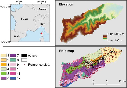
The Asco Valley is located on the French island of Corsica and covers 16,574 ha, with elevation that ranges from 195–2670 m (Figure 1). This study site has a granite substrate and includes three climates (Mediterranean, high Mediterranean, and alpine) that, combined with agricultural practices and fires, shape the vegetation’s distribution (Gamisans et al. 1981). The region is characterized by severe summer drought from June to September and several months of snowfall at the highest elevations from December to April. Hence, vegetation in the Asco Valley has high floristic richness (Delbosc, Bioret, and Panaiotis 2015), as indicated by the presence of two protected Natura 2000 sites.

Figure 1. Study site location, elevation map, and data used for the study. Numbers in the bottom legend refer to the 12 vegetation series (see Table 1 for definitions). “Others” represents vegetation series along streams and among rock falls, covering less than 5% of the study site.

Field-based map of vegetation series

A map of the vegetation series of the Asco Valley at the 1:25 000 scale was produced in 2012 by Delbosc, Bioret, and Panaiotis (2015) combining thematic layers and phytosociological field observations as follows: (i) tessela – environmentally homogeneous units that shaped the contours of each vegetation series – were delineated using the approach of Blasi, Capotorti, and Frondoni (2005) based on environmental variables (geological, climate, topographical, and soil maps); (ii) the abundance of each syntaxon within a tessela was observed in landscape vegetation in the field from April to August 2012 according to the Rivas-Martinez approach (2005); (iii) all landscape vegetation observations (n = 261) were categorized according to their syntaxonomic composition, which classified vegetation series and characterized their topo-climatic attributes; and (iv) each tessela was assigned to a vegetation series depending on its topo-climatic properties. The full methodology is described in Delbosc, Bioret, and Panaiotis (2017). A detailed floristic composition of each vegetation series is presented in Appendix 1.

Satellite data

MODIS satellite images were evaluated to map the 12 vegetation series. To obtain cloud-free images, the MOD13Q1 product, which contains the best pixel available from all acquisitions made over a 16-day period (Solano et al. 2010), was selected. The MOD13Q1 product has spectral bands in the red (620–670 nm) and near-infrared (NIR) (841–876 nm) wavelengths and 250 m spatial resolution. A time-series of 24 MODIS images for an annual vegetation cycle (1 November 2014 to 31 October 2015) was downloaded for free from NASA’s Earthdata search platform (https://search.earthdata.nasa.gov/) and projected onto the French projection system (Lambert RGF93) using the MODIS reprojection tool. For each date, NDVI was derived from the ratio between the red and NIR spectral bands. All MODIS time-series red, NIR, and NDVI bands (n = 3 × 24) were compiled into a single raster file for the classification process.

Methods

The structural and functional mapping method consisted of six steps (Figure 2).

Figure 2. Methodological flowchart.

Structural mapping

Step 1 sampling

This step selected which MODIS pixels to use to calibrate the random forest (RF) model. MODIS raster data were overlaid with the field-based vector map of the vegetation series in a GIS environment (QGIS 2018). Some vegetation series with a small area – representing less than 5% of the study site and located along streams and among rock falls (Figure 1) – were excluded because they were considered too small given the spatial resolution of the MODIS images. Thus, the 12 vegetation series that covered the largest areas were considered in this study (Table 1). To remove mixed pixels, only those contained entirely within a tessela were selected as reference plots. To limit the effect of class imbalance, which could decrease the performance of the classification algorithm (Maxwell, Warner, and Fang 2018), reference plots were limited to 50 per vegetation series (Table 1). The spectral values of red, NIR, and NDVI band were then assigned to each reference plot. Then, spectral values of the reference plots were scaled.

Table 1. Classification and number of reference plots for each vegetation series (see Table S1 for a detailed description of vegetation series).

Code	No. plots	Vegetation series name
1	50	Galio scabri-Querco illicis sigmetum variant with Lathyrus venetus
2	16	Buxo sempervirentis-Querco ilicis sigmetum
3	15	Stachyo glutinosae-Genisto corsicae minorisigmetum variant with Juniperus oxycedrus
4	50	Junipero oxycedri-Querco ilicis sigmetum
5	47	Galio rotundifolii-Pino laricii sigmetum variant with Erica arborea
6	50	Galio rotundifolii-Pino laricii sigmetum variant with Luzula pedemontana
7	28	Festuco sardoae-Phyteumo serrati geopermasigmetum
8	18	Paronychio polygonifoliae-Armerio multicepitis minorisigmetum
9	46	Sorbo aucupariae-Acero pseudoplatani sigmetum
10	19	Geo montani-Phleo brachystachyi geopermasigmetum
11	14	Valeriano rotundifoliae-Adenostylo briquetii geopermasigmetum
12	17	Acino corsici-Tanaco tomentosi geopermasigmetum
Total	380

Step 2 measure the importance of image date

This step measured the importance of each MODIS image in discriminating vegetation series. An RF model was applied to red, NIR, and NDVI bands in the MODIS time-series and calibrated from the reference plots. Compared to other models, RF has the advantage of avoiding redundant variables by selecting the most discriminating spectral band during classification (Rodriguez-Galiano et al. 2012). More precisely, RF iteratively switches one MODIS band while keeping the others constant and then measures the decrease in the normalized Gini index (Breiman 2001), for which the sum of all MODIS bands indices equaled one. For each date, normalized Gini index values for the red, NIR, and NDVI bands were summed.

Step 3 calculates the optimal number of dates

This step identified how many MODIS dates could be removed without decreasing the accuracy of the RF model. The RF model was iteratively run 24 times, and the least important date in the MODIS time-series was removed at each iteration. In detail, the RF model was calibrated and validated based on reference plots using three repeated fivefold cross-validation (Kuhn 2008). Specifically, the original reference plots were randomly split into k samples, one of the k samples was selected as the validation set, and the k-1 other samples constituted the calibration set. The performance score was calculated and then repeated by selecting another validation sample from among the k-1 samples that had not yet been used for model validation. The operation was performed k times so that in the end each sub-sample was used exactly once as a validation set. To obtain a more robust estimate of RF model performance, the k-fold process was repeated three times. The RF model accuracy was determined using the kappa index that expresses the proportional reduction in error generated by a classification process compared with the error of a completely random classification (Congalton, Oderwald, and Mead 1983). The Kappa index is commonly used for the assessment of prediction errors in machine learning classification (Ben-David 2008; Maxwell, Warner, and Fang 2018), since it is an overall statistical agreement of a confusion matrix, including non-diagonal values (Lu and Weng 2007) and a suitable index for imbalanced class datasets (Nguyen, Bouzerdoum, and Phung 2008). A median Kappa index and a median overall accuracy with their respective standard deviations were calculated iteratively based on the three repeated fivefold cross-validation procedure. Next, RF model accuracy was plotted as a function of the number of dates selected, and the optimal number of dates was that with the largest median Kappa index.

Step 4 MODIS modeling

This step automatically mapped the vegetation series using the red, NIR, and NDVI bands of the MODIS time-series. The model, previously calibrated using the optimal number of dates, was applied to all pixels of the MODIS time-series. A fivefold cross-validated confusion matrix was calculated that represented the error distribution per vegetation series among the three repeats.

Functional mapping

Step 5 calculate functional indices

This step mapped functional processes expressed by vegetation using the NDVI biophysical variable from MODIS time-series. Specifically, three functional indicators were derived from the annual NDVI curve (Alcaraz, Paruelo, and Cabello 2006): (i) the annual NDVI integral (NDVI-I), equal to the sum of NDVI, which represents net primary production (Pettorelli et al. 2005); (ii) the intra-annual relative range (RREL), calculated as maximum NDVI minus minimum NDVI, divided by NDVI-I, that describes the seasonality of carbon fluxes (Cabello et al. 2012); and (iii) the date of annual maximum NDVI (MMAX), that features for vegetation phenology (Weber, Schaepman-Strub, and Ecker 2018). As the NDVI values of MODIS images are negative on the snow cover (Beck et al. 2006), these pixels were reclassified to zero to avoid any bias in the calculation of the functional indices.

Step 6 constrained ordination

This step summarized the three functional indicators into a synthetic two-dimensional space. For each reference plot, the values of the three functional indices were extracted in a GIS environment. Next, reference plots of the vegetation series were ordinated according to a normalized principal component analysis (PCA). The influence of vegetation series on the functional variance was tested using between-class component analysis, which is a particular case of PCA that emphasizes differences between groups (here, vegetation series) (Dray and Dufour 2007). Based on this analysis, between-class inertia is the percentage of total PCA inertia explained by vegetation series.

Results

Variable importance

The importance of the red, NIR, and NDVI bands of the MODIS time-series used in the RF model indicated that some seasons were more discriminating than others, particularly late winter to early spring (10 February to 15 April 2015) (Figure 3), which showed a normalized decrease in Gini index values of 0.050–0.075. To a smaller extent, MODIS images acquired in spring and summer (17 May to 5 August 2015) were also discriminating, with decreases of 0.038–0.050. Conversely, late summer, autumn, and early winter (8 October 2014 to 25 January 2015, and 21 August to 8 October 2015) were the least discriminating, with decreases of 0.026–0.034. In addition, the relative importance of each spectral band varied throughout the year. The NDVI band was the most discriminating during autumn and winter (8 October 2014 to 14 March 2015, and 6 September to 8 October 2015). Conversely, the NIR band was the most discriminating in spring and summer (15 April to 21 August 2015), while the red band was the most discriminating only on 30 March 2015.

Figure 3. Decrease in the normalized Gini index (the sum of all spectral variable indices equaled one) for each spectral band obtained from the random forest classifier; larger values indicate greater importance.

Optimal number of MODIS images

RF model accuracy as a function of the number of MODIS images selected (Figure 4) indicated a higher value with the 18 best MODIS dates (median Kappa index 0.70 ± 0.05, median overall accuracy 0.76 ± 0.04). The six dates not selected corresponded mainly to late summer and autumn (8 and 24 October, 9 November 2020 July, 6 and 22 September). Furthermore, the RF model had similar accuracy (median Kappa index 0.67 ± 0.05, median overall accuracy 0.73 ± 0.03) when selecting the 10 best dates, corresponding to late winter and spring (25 January 2010 and 26 February 2014 and 30 March 2015 April, 17 May, 2 and 18 June, 5 August). Conversely, the RF model had much lower accuracy when less than 10 dates were selected (e.g. median Kappa index 0.55, median overall accuracy 0.61 using six dates and median Kappa index 0.38, overall accuracy 0.45 using one date). Notably, the standard deviation of model accuracy remained low and relatively constant for the Kappa index (0.04–0.07) as well as the overall accuracy (0.04–0.08) regardless of the number of dates selected.

Figure 4. Modeling accuracy (median Kappa index) as a function of the number of dates selected (ranked in decreasing order of importance). The gray area indicates the standard deviation, while the vertical dotted line indicates the number of dates selected for the final RF model.

Map of vegetation series

The map of vegetation series was derived from the RF model using the 18 most important dates in the MODIS time-series (median Kappa index 0.70 ± 0.05, median overall accuracy 0.76 ± 0.04). A cross-validated confusion matrix described the classification accuracy for each vegetation series and the distribution of classification errors (Table 2). Producer’s accuracy was high (71–100%) for all vegetation series except for series 6, 9, and 10, which had moderate values (64–69%). User’s accuracy was high (75–93%) for vegetation series 1, 4, 6, 9, and 12; moderate (51–67%) for series 2, 5, 7, and 10; and low (42–50%) for series 3, 8, and 11.

Table 2. Cross-validated (fivefold, repeated three times) confusion matrix between the modeling of 12 vegetation series derived from the MODIS time-series (rows) and the validation reference plots (columns). Entries are total cell counts across resamples.

		Reference
Modeling	Code	1	2	3	4	5	6	7	8	9	10	11	12	User’s accuracy (%)
Galio scabri-Querco illicis sigmetum variant with Lathyrus venetus	1	140	2		8									93
Buxo sempervirentis-Querco ilicis sigmetum	2	12	31		5									65
Stachyo glutinosae-Genisto corsicae minorisigmetum variant with Juniperus oxycedrus	3	6		19	12	3		5						42
Junipero oxycedri-Querco ilicis sigmetum	4	20	3		124	3								83
Galio rotundifolii-Pino laricii sigmetum variant with Erica arborea	5				18	95	25	3						67
Galio rotundifolii-Pino laricii sigmetum variant with Luzula pedemontana	6				2	23	112	7	4	2				75
Festuco sardoae-Phyteumo serrati geopermasigmetum	7				8	10	13	48		3	2			57
Paronychio polygonifoliae-Armerio multicepitis minorisigmetum	8						7		24	23				44
Sorbo aucupariae-Acero pseudoplatani sigmetum	9						5		3	120	6	3	1	87
Geo montani-Phleo brachystachyi geopermasigmetum	10						1			16	29	1	10	51
Valeriano rotundifoliae-Adenostylo briquetii geopermasigmetum	11						6		2	7		21	6	50
Acino corsici-Tanaco tomentosi geopermasigmetum	12									2	8		41	80
Producer’s accuracy (%)		79	86	100	70	71	66	76	73	69	64	84	71

Compared to the reference map (Figure 1), the MODIS time-series modeling (Figure 5(a)) showed great similarity in the spatial distribution of vegetation series. Specifically, the reference and MODIS-derived maps highlighted the elevation gradient from the Mediterranean vegetation series (1–7) in the valley bottom to the sub-alpine (8–11) and alpine (12) series at mountain tops.

Figure 5. (a) Structural and (b) functional maps of vegetation series derived from the MODIS satellite images. Numbers in the legend refer to the 12 vegetation series (see Table 1 for definitions).

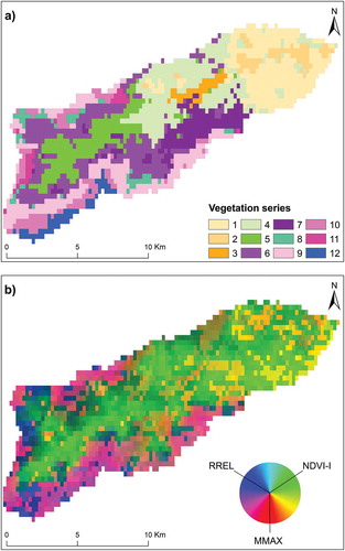
Functional dimension of vegetation series

The functional map based on a color composite of the three indices (NDVI-I, RREL, and MMAX) (Figure 5(b)) revealed a topo-climatic gradient ranging from (i) Mediterranean vegetation series (1–7) with high NDVI-I (10.7–15.9), low RREL (0.01–0.05), and low MMAX (25 January-30 March), indicative of high annual net primary production, a weak seasonal pattern of carbon flux, and early phenology, respectively; to (ii) sub-alpine and alpine vegetation series (8–12) with low NDVI-I (2.5–8.0), high RREL (0.08–0.13), and high MMAX (14 March-4 July), indicative of low annual net primary production, a strong seasonal pattern of carbon flux, and late phenology, respectively.

In the two-dimensional space for the vegetation series derived from the PCA (Figure 6), the first two PCA axes explained 96% of the variance in the three functional indices. Axis 1 (68% of total variance) was negatively correlated with NDVI-I (−0.95) and positively correlated with RREL (0.93), while axis 2 (28% of total variance) was positively correlated with MMAX (0.86). The ordination diagram supported the existence of a topo-climatic gradient from the Mediterranean series (1–7) (Figure 6, left), with high NDVI-I, to the sub-alpine and alpine series (8–12) (Figure 6, right), with high RREL. Although a topo-climatic gradient was identified, the 12 vegetation-series explained no more than 60% (i.e. between-class variance, p < 0.001) of total variance for the three functional indices, suggesting high functional variance within each vegetation series. These results were confirmed by visual inspection of the diagram, which emphasized an overlap of confidence ellipses.

Figure 6. Ordination diagram of principal component analysis (PCA). Vectors show the direction and importance of functional indices. Confidence ellipses (p = 0.9) are drawn around the barycenters of vegetation series, each of which is represented by a code number. Mediterranean vegetation series are black, while sub-alpine and alpine vegetation series are gray.

Discussion

It is possible to discriminate vegetation series with various physiognomies spectrally from an annual satellite time-series at a coarse spatial resolution

This study demonstrates that MODIS images at a coarse spatial resolution are well suited for mapping 12 Mediterranean vegetation series with various physiognomies (median Kappa index 0.70, median overall accuracy 0.76). These results are consistent with those of the initial application to Atlantic marshes (Rapinel et al. 2018) and highlight the transferability of the approach to other natural environments. While the coarse spatial resolution of MODIS images can be considered inadequate for mapping natural vegetation (Corbane et al. 2015), the present study indicates that it is suitable for mapping vegetation series, since each pixel summarizes the floristic composition of vegetation in the landscape, which is an indicator of natural habitats and their conservation status (Rodwell, Evans, and Schaminée 2018). For example, the Paronychio polygonifoliae-Armerio multicepitis minori sigmetum series, which was spatialized by RF classification to areas above 2 000 m (Figure 2), was defined by two plant communities (Paronychio polygonifoliae-Armerietum multicepitis armerietosum multicepitis and Paronychio polygonifoliae-Armerietum multicepitis genistetosum lobeloidis), which are indicators for EUNIS habitats E4.37 Oro-Corsican grassland and F7.4 Hedgehog-heaths, respectively.

It is important to recall, however, that some vegetation series covering small areas, such as those along streams or in rock falls, were not mapped in this study because their spatial extent was considered too small in relation to the coarse spatial resolution of the MODIS images (Figure 1). Even though these series cover less than 5% of the area, they may have high biodiversity. Compared to deductive mapping of vegetation series based on analysis of topo-climatic variables (Blasi, Capotorti, and Frondoni 2005), the satellite-image approach provides continuous observation of vegetation. These results, however, had approximately 30% error in mapping (Table 2). Combining topo-climatic variables and satellite images could increase the modeling accuracy of vegetation series.

As expected, the confusion matrix (Table 2) highlighted that most classification errors occurred between neighboring and ecologically similar vegetation series (Delbosc, Bioret, and Panaiotis 2015), such as between the Galio rotundifolii-Pino laricii sigmetum variant with Erica arborea (series 5) and variant with Luzula pedemontana (series 6). In addition, some vegetation series with small areas (3, 8, 10, and 11) were classified with high producer’s accuracy but low user’s accuracy (Table 2). These errors may be explained by the sampling: although class imbalance was minimized (Table 1), RF model machine-learning increases overall accuracy at the expense of under-represented classes, which have less impact on overall accuracy than other classes (Maxwell, Warner, and Fang 2018). Yet, these four series were calibrated with a small number of reference plots (14–19) due to their small area, given the coarse size of a MODIS pixel. However, satellite images with a fine spatial resolution, such as Sentinel-2 (10 m), appear more appropriate for mapping plant associations (Rapinel et al. 2019; Shoko and Mutanga 2017) than for mapping vegetation series. Alternatively, satellite images with a medium spatial resolution, such as Landsat (30 m), have the most suitable spatial resolution to map all vegetation series (Rapinel et al. 2015), but their low temporal resolution (1–2 cloud-free images per year) is not sufficient for functional characterization.

The RF classification map based on MODIS images correlated well with the field map, although the field map looked better since its vegetation series were manually delimited at 1:25 000. Conversely, the vegetation series map derived from MODIS data was extracted automatically from RF classification of pixels at 250 m, resulting in “salt-and-pepper” and “stair-step” artifacts. These are observed most frequently between spatially adjacent or interspersed vegetation series whose edges the coarse spatial resolution of MODIS data cannot clearly discriminate due to mixed pixels (Lu and Weng 2007), such as between the Sorbo aucupariae-Acero pseudoplatani sigmetum (series 9) and the Geo montani-Phleo brachystachyi geopermasigmetum (series 10). An additional filtering-based processing step would reduce these artifacts to improve the appearance of the classification (Huang et al. 2014).

It should be kept in mind, however, that good looking map is not always a good map (Perennou et al. 2018): while the accuracy of the MODIS RF classification was assessed, that of the field map was not, which is a common issue for natural vegetation (Borre et al. 2011). Although the field map looked good, it may have contained errors due not only to field workers’ subjective interpretations but also to the coarse resolution of environmental variables used as ancillary data (e.g. geological or topographical maps) (Ullerud et al. 2018). This has an impact on the quality of the field samples and therefore on the modeling accuracy (Foody et al. 2016). This issue can be addressed by detecting and removing poor quality samples from the dataset using methods based on mahalanobis distance (Liu, White, and Newell 2018), fuzzy c-means classifier (Duff, Bell, and York 2014), or RF proximity distance (Raab et al. 2018).

The respective influences of date and spectrum on modeling accuracy

The temporal resolution of the MOD13Q1 product (16 days) is well suited for discriminating vegetation series. Indeed, using time-series increases detection of vegetation units (Stenzel et al. 2014) and helps characterize phenology or ecological variables that shape the distribution of vegetation units, such as snow cover duration. At least 10 MODIS acquisition dates are essential for sufficient accuracy (Figure 4), however, compared to two for Landsat (Rapinel et al. 2015): this emphasizes that the coarse spatial resolution of MODIS images can be compensated by its high time resolution. Moreover, RF classification revealed that images acquired in late winter and early summer were more important in discriminating vegetation series than those acquired in late summer and autumn. More specifically, the RF model’s accuracy peaked when using 18 dates; the remaining six dates corresponding to late summer and autumn can be considered noise since they slightly decreased the model’s accuracy (Figure 4). These results support that even though the RF model is suited for high-dimension feature space, removing the least important variables can increase overall accuracy (Maxwell, Warner, and Fang 2018).

The NDVI band – which has discriminating negative values for snow cover (Beck et al. 2006) – was more important than the NIR band during autumn and winter, unlike during the rest of the year (Figure 3), suggesting that vegetation series are discriminated based on snow cover duration, which is a function of elevation and exposure. Summer is also an important season for discriminating vegetation series on the basis of the NIR band. In the Mediterranean series, some plant communities can be senescent due to water stress, while in the alpine series, plant communities are growing rapidly (Gamisans 1977). Since previous studies have highlighted the potential of elevation and exposure variables to map vegetation series (Biondi, Casavecchia, and Pesaresi 2011), the combination of topo-climatic variables with spectral variables would likely increase not only the accuracy but also the robustness of the model for application over larger areas.

It is possible to identify a functional gradient in these vegetation series

Comparison of the structural and functional maps identified a gradient ranging from high annual net primary production with low seasonality of carbon fluxes and early phenology in the Mediterranean series to low annual net primary production with high seasonality of carbon fluxes and late phenology in alpine series. This functional gradient may be explained by differences in vegetative activity among vegetation series in Corsica: the Mediterranean series are composed essentially of sclerophyllous plant communities (e.g. Galio scabri-Quercetum ilicis lathyretosum veneti, Galio rotundifolii-Pinetum laricii ericetosum arboreae) that produce biomass throughout the year (Gamisans 1977). Conversely, alpine vegetation series are composed not only of deciduous tree plant communities (Sorbo aucupariae-Aceretum pseudoplatani), whose photosynthetic activity is limited to the June–August period, but also of lawns and heath plant communities that are dormant in winter and spring because of snow cover (Jeanmonod and Gamisans 2013). On the other hand, the results also point to functional variance within each vegetation series (Figures 5 and 6), indicating the value of both structural and functional maps for managing plant biodiversity (Cabello et al. 2012; Requena-Mullor et al. 2018). The functional variance observed within each series could be explained by local differences in facies (dominant plant species) and/or short-term response related to environmental stresses such as grazing (Alrababah et al. 2007) or drought (Nogueira et al. 2017).

Conclusion

This study highlights that 12 vegetation series in the Mediterranean region can be discriminated using annual time-series of satellite images at a coarse spatial resolution (250 m) and RF modeling. At least 10 images are required to achieve sufficient accuracy, suggesting that the coarse spatial resolution of MODIS data can be compensated by its high time resolution. Comparison of structural and functional maps identified a functional gradient, ranging from high annual net primary production with low seasonality of carbon fluxes and early phenology in the Mediterranean series to low annual net primary production with high seasonality of carbon fluxes and late phenology in alpine series. Ongoing methodological challenges include (i) improving the cartographic scale by integrating future monthly cloud-free Sentinel-2 syntheses (20 m); (ii) improving classification accuracy and robustness by combining satellite images with topo-climatic variables; and (iii) evaluating the classification model on larger areas.

Highlights

• We evaluated a MODIS time-series to map natural vegetations in the Mediterranean region.

• We described vegetation-series along structural and functional dimensions.

• We compared the influence of reducing MODIS time-series on classification accuracy.

• RF classification reached an overall accuracy of 0.76 using images from February to August.

• A minimum of 10 MODIS acquisitions is required to get correct accuracy.

• A functional gradient from the Mediterranean to alpine vegetation is revealed.

Acknowledgements

This study was supported by the French Ministry of Ecology (CarHAB program) under grant no. 2101606295. MODIS data were retrieved from the EOSDIS Land Processes Distributed Active Archive Center (LP DAAC), USGS/Earth Resources Observation and Science (EROS). We thank the Conservatoire Botanique National de Corse for providing the field-based vegetation maps.

Disclosure statement

No potential conflict of interest was reported by the authors.

Additional information

Funding

This work was supported by the Ministère de la Transition écologique et Solidaire [2101606295].

Appendix

Table

	Code		1	2	3	4	5	6	7	8	9	10	11	12
	Physio-gnomy*	CORINE Biotopes
Plant communities of mesomediterranean belt
Galio scabri-Quercetum ilicis lathyretosum veneti	f	45.316	I	.	.	.	.	.	.	.	.	.	.	.
Buxo sempervirentis-Quercetum ilicis	f	45.3	.	II	.	.	.	.	.	.	.	.	.	.
Cyclamino repandi-Phillyreetum latifoliae	f	45.14	.	.	.	.	.	.	.	.	.	.	.	.
Pulicario odorae-Arbutetum unedonis	s	32.3	III	I	.	.	.	.	.	.	.	.	.	.
Pulicario odorae-Arbutetum unedonis phillyreetosum latifoliae	s	32.3	II	II	.	.	.	.	.	.	.	.	.	.
Pulicario odorae-Arbutetum unedonis pinetosum hamiltonii	f	42.82	I	.	.	.	.	.	.	.	.	.	.	.
Helichryso italici-Cistetum cretici	h	32.3	II	V	.	.	.	.	.	.	.	.	.	.
Stachydo glutinosae-Genistetum corsicae teucrietosum mari	h	32.482	I	.	.	.	.	.	.	.	.	.	.	.
Stachydo glutinosae-Genistetum corsicae juniperetosum oxycedrus subsp. oxycedrus	h	32.482	.	.	IV	.	.	.	.	.	.	.	.	.
Stachydo glutinosae-Genistetum corsicae	h	32.482	IV	II	V	.	.	.	.	.	.	.	.	.
Stachydo glutinosae-Genistetum corsicae rosmarinetosum officinalis	h	32.482	.	.	II	.	.	.	.	.	.	.	.	.
Tuberario guttatae-Plantaginetum bellardii	l	35.21	V	V	IV	.	.	.	.	.	.	.	.	.
Plant communities with Chenopodium vulvaria and Urtica urens	l	87	I	I	.	.	.	.	.	.	.	.	.	.
Plant communities of supramediterranean belt
Junipero oxycedrii-Quercetum ilicis	f	45.322	.	.	.	V	.	.	.	.	.	.	.	.
Galio rotundifolii-Pinetum laricii ericetosum arboreae	f	42.643	.	.	.	.	V	.	.	.	.	.	.	.
Helichryso italici-Genistetum salzmannii	h	31.754	.	.	.	V	V	.	.	.	.	.	.	.
Caricion caryophyllae	l	36.37	.	.	.	V	IV	.	.	.	.	.	.	.
Plant communities of moutainous-oromediterranean belt
Galio rotundifolii-Pinetum laricii lusuletosum pedemontanae	f	42.641	.	.	.	.	.	I	.	.	.	.	.	.
Galio rotundifolii-Pinetum laricii plant communities with Betula pendula	f	42.64	.	.	.	.	.	I	.	.	.	.	.	.
Galio rotundifolii-Pinetum laricii anthyllidetosum hermaniae	f	42.642	.	.	.	.	.	V	.	.	.	.	.	.
Berberido aetnensis-Genistetum lobelioidis	h	31.75	.	.	.	.	.	V	.	.	.	.	.	.
Thymo herba-baronae-Genistetum lobelioidis	h	31.7	.	.	.	.	.	III	.	.	.	.	.	.
Anthoxantho odorati-Brachypodietum pinnati	l	36.371	.	.	.	.	.	I	.	.	.	.	.	.
Sagino piliferae-Caricetum caryophylleae	l	36.371	.	.	.	.	.	I	.	.	.	.	.	.
Festuco sardoae-Phyteumetum serrati permasigmetum	l	62.2	.	.	.	.	.	.	V	.	.	.	.	.
Plant communities with Cerastium soleirolii	l	62.2	.	.	.	.	.	.	IV	.	.	.	.	.
Potentillion crassinerviae	l	62.2	.	.	.	.	.	.	IV	.	.	.	.	.
Plant communities of cryo-oromediterranean belt
Paronychio polygonifoliae-Armerietum multicepitis armerietosum multicepitis	l	36.371	.	.	.	.	.	.	.	V	.	.	.	.
Paronychio polygonifoliae-Armerietum multicepitis genistetosum lobeloidis	h	31.7	.	.	.	.	.	.	.	V	.	.	.	.
Plant communities of subalpine belt
Sorbo aucupariae-Aceretum pseudoplatani	f	31.612	.	.	.	.	.	.	.	.	V	.	.	.
Alnetum suaveolentis alnetosum suaveolentis	h	31.612	.	.	.	.	.	.	.	.	V	.	.	.
Plant communities with Juniperus alpina subsp. nana	h	31.75	.	.	.	.	.	.	.	.	IV	.	.	.
Valeriano rotundifoliae-Adenostylo briquetii permasigmetum	l	37.85	.	.	.	.	.	.	.	.	.	.	V	.
Dryopteridi oreadi-Arrhenathero sardoi permasigmetum	l	61.11	.	.	.	.	.	.	.	.	.	.	III	.
Geo montani-Phleetum brachystachyi	l	36.374	.	.	.	.	.	.	V	.	II	V	.	.
Huperzio selaginis-Carico ornithopodae permasigmetum		36.374	.	.	.	.	.	.	.	.	.	I	.	.
Pinguiculo corsicae-Trichophoretum cespitosi permasigmetum	l	54.455	.	.	.	.	.	.	.	.	.	V	.	.
Plant communities of alpine belt			.	.	.	.	.	.	.	.	.	.	.	.
Acino corsici-Tanaceto tomentosi permasigemtum	l	36.373	.	.	.	.	.	.	.	.	.	.	.	V
Asplenio viridi-Drabo dubiae permasigemtum	l	62.2	.	.	.	.	.	.	.	.	.	.	.	V
Gnaphalio supini-Sibbaldio procumbentis permasigmetum	l	36.374	.	.	.	.	.	.	.	.	.	.	.	V
Anthropogenic plant communities
Pruno spinosae-Rubion ulmifolii	h	31.8	I	.	.	.	.	I	.	.	.	.	.	.
Pruno spinosae-Rubion ulmifolii plant communities with Rubus ulmifolius and Prunus spinosa	h	31.8	I	I	.	.	III	I	.	.	.	.	.	.
Pruno spinosae-Rubion ulmifolii plant communities with Pteridium aquilinum	h	31.8	II	III	.	I	.	.	.	.	.	.	.	.
Echio lycopsis-Galactitetum tomentosae	l	87	II	II	.	IV	.	.	.	.	.	.	.	.
Onopordetum illyrici	l	32.9	.	.	.	I	.	.	.	.	.	.	.	.

References

- Alcaraz, D., J. Cabello, and J. Paruelo. 2009. “Baseline Characterization of Major Iberian Vegetation Types Based on the NDVI Dynamics.” Plant Ecology 202 (1): 13–29. doi:10.1007/s11258-008-9555-2.
- Alcaraz, D., J. Paruelo, and J. Cabello. 2006. “Identification of Current Ecosystem Functional Types in the Iberian Peninsula.” Global Ecology and Biogeography 15 (2): 200–212. doi:10.1111/j.1466-822X.2006.00215.x.
- Alrababah, M. A., M. A. Alhamad, A. Suwaileh, and M. Al‐Gharaibeh. 2007. “Biodiversity of Semi-Arid Mediterranean Grasslands: Impact of Grazing and Afforestation.” Applied Vegetation Science 10 (2): 257–264. doi:10.1111/j.1654-109X.2007.tb00524.x.
- Beck, P. S. A., C. Atzberger, K. Arild Høgda, B. Johansen, and A. K. Skidmore. 2006. “Improved Monitoring of Vegetation Dynamics at Very High Latitudes: A New Method Using MODIS NDVI.” Remote Sensing of Environment 100 (3): 321–334. doi:10.1016/j.rse.2005.10.021.
- Ben-David, A. 2008. “Comparison of Classification Accuracy Using Cohen’s Weighted Kappa.” Expert Systems with Applications 34 (2): 825–832. doi:10.1016/j.eswa.2006.10.022.
- Biondi, E., S. Casavecchia, and S. Pesaresi. 2011. “Phytosociological Synrelevés and Plant Landscape Mapping: from Theory to Practice.” Plant Biosystems-An International Journal Dealing with All Aspects of Plant Biology 145 (2): 261–273. doi:10.1080/11263504.2011.572569.
- Blasi, C., G. Capotorti, and R. Frondoni. 2005. “Defining and Mapping Typological Models at the Landscape Scale.” Plant Biosystems-An International Journal Dealing with All Aspects of Plant Biology 139 (2): 155–163. doi:10.1080/11263500500163629.
- Borre, J. V., D. Paelinckx, C. A. Mücher, L. Kooistra, B. Haest, G. De Blust, and A. M. Schmidt. 2011. “Integrating Remote Sensing in Natura 2000 Habitat Monitoring: Prospects on the Way Forward.” Journal for Nature Conservation 19 (2): 116–125. doi:10.1016/j.jnc.2010.07.003.
- Breiman, L. 2001. “Random Forests.” Machine Learning 45 (1): 5–32. doi:10.1023/A:1010933404324.
- Cabello, J., N. Fernández, D. Alcaraz-Segura, C. Oyonarte, G. Piñeiro, A. Altesor, M. Delibes, and J. M. Paruelo. 2012. “The Ecosystem Functioning Dimension in Conservation: Insights from Remote Sensing.” Biodiversity and Conservation 21 (13): 3287–3305. doi:10.1007/s10531-012-0370-7.
- Clerici, N., C. J. Weissteiner, and F. Gerard. 2012. “Exploring the Use of MODIS NDVI-Based Phenology Indicators for Classifying Forest General Habitat Categories.” Remote Sensing 4 (6): 1781–1803. doi:10.3390/rs4061781.
- Congalton, R. G., R. G. Oderwald, and R. A. Mead. 1983. “Assessing Landsat Classification Accuracy Using Discrete Multivariate Analysis Statistical Techniques.” Photogrammetric Engineering and Remote Sensing 49: 1671–1678.
- Corbane, C., S. Lang, K. Pipkins, S. Alleaume, M. Deshayes, V. E. García Millán, T. Strasser, J. Vanden Borre, T. Spanhove, and M. Förster. 2015. “Remote Sensing for Mapping Natural Habitats and Their Conservation Status – New Opportunities and Challenges.” International Journal of Applied Earth Observation and Geoinformation, Special Issue on Earth Observation for Habitat Mapping and Biodiversity Monitoring 37 (May): 7–16. doi:10.1016/j.jag.2014.11.005.
- Council Directive 92/43/EEC. 1992. “Conservation of Natural Habitats and of Wild Flora and Fauna.” International Journal of the European Communities L206: 7–49.
- Delbosc, P., F. Bioret, and C. Panaiotis. 2015. “Vegetation Series of Ascu Valley (corsica), Typology and Map at 1:25 000.” Ecologia Mediterranea 41 (1): 5–87.
- Delbosc, P., F. Bioret, and C. Panaiotis. 2017. “Dynamic-Catenal Phytosociological Mapping of Corsica: Inductive Methodological Approach.” Contributii Botanice 52: 29–54.
- Dray, S., and A. B. Dufour. 2007. “The Ade4 Package: Implementing the Duality Diagram for Ecologists.” Journal of Statistical Software 22 (4): 1–20. doi:10.18637/jss.v022.i04.
- Duff, T. J., T. L. Bell, and A. York. 2014. “Recognising Fuzzy Vegetation Pattern: the Spatial Prediction of Floristically Defined Fuzzy Communities Using Species Distribution Modelling Methods.” Journal of Vegetation Science 25 (2): 323–337. doi:10.1111/jvs.12092.
- Ellwanger, G., S. Runge, M. Wagner, W. Ackermann, M. Neukirchen, W. Frederking, C. Müller, A. Ssymank, and U. Sukopp. 2018. “Current Status of Habitat Monitoring in the European Union according to Article 17 of the Habitats Directive, with an Emphasis on Habitat Structure and Functions and on Germany.” Nature Conservation 29 (October): 57–78. doi:10.3897/natureconservation.29.27273.
- Foody, G. M., M. Pal, D. Rocchini, C. X. Garzon-Lopez, and L. Bastin. 2016. “The Sensitivity of Mapping Methods to Reference Data Quality: Training Supervised Image Classifications with Imperfect Reference Data.” ISPRS International Journal of Geo-Information 5 (11): 199. doi:10.3390/ijgi5110199.
- Gamisans, J. 1977. “La Végétation Des Montagnes Corses.” Phytocoenologia 4: 133–179.
- Gamisans, J., M. Gruber, J. Claudin, and J. B. Casanova. 1981. “Carte de La Végétation Du Haut-Vénecais Au 1/25 000.” Ecologia Mediterranea 7 (1): 85–98.
- Gigante, D., A. T. R. Acosta, E. Agrillo, S. Armiraglio, S. Assini, F. Attorre, S. Bagella, G. Buffa, L. Casella, and C. Giancola. 2018. “Habitat Conservation in Italy: the State of the Art in the Light of the First European Red List of Terrestrial and Freshwater Habitats.” Rendiconti Lincei. Scienze Fisiche E Naturali 29: 1–15.
- Hagolle, O., D. Morin, and M. Kadiri. 2018. “Detailed Processing Model for the Weighted Average Synthesis Processor (WASP) for Sentinel-2.” August. doi:10.5281/zenodo.1401360.
- Huang, X., Q. Lu, L. Zhang, and A. Plaza. 2014. “New Postprocessing Methods for Remote Sensing Image Classification: A Systematic Study.” IEEE Transactions on Geoscience and Remote Sensing 52 (11): 7140–7159. doi:10.1109/TGRS.2014.2308192.
- Janssen, J. A. M., J. S. Rodwell, M. García Criado, G. H. P. Arts, R. J. Bijlsma, and J. H. J. Schaminee. 2016. European Red List of Habitats. European Union, Luxembourg.
- Jeanmonod, D., and J. Gamisans. 2013. “Flora Corsica. 2nd Rev and Augmented Edition.” Bulletin de La Société Botanique. Centre-Ouest, No Spécial 39: 1074.
- Kuhn, M. 2008. “Caret Package.” Journal of Statistical Software 28 (5): 1–26.
- Liu, C., M. White, and G. Newell. 2018. “Detecting Outliers in Species Distribution Data.” Journal of Biogeography 45 (1): 164–176. doi:10.1111/jbi.13122.
- Lu, D., and Q. Weng. 2007. “A Survey of Image Classification Methods and Techniques for Improving Classification Performance.” International Journal of Remote Sensing 28 (5): 823–870. doi:10.1080/01431160600746456.
- Maxwell, A. E., T. A. Warner, and F. Fang. 2018. “Implementation of Machine-Learning Classification in Remote Sensing: an Applied Review.” International Journal of Remote Sensing 39 (9): 2784–2817. doi:10.1080/01431161.2018.1433343.
- Nguyen, G. H., A. Bouzerdoum, and S. L. Phung. 2008. “A Supervised Learning Approach for Imbalanced Data Sets.” In 2008 19th International Conference on Pattern Recognition, IEEE, Tampa, Florida, USA, 1–4.
- Nogueira, C., M. N. Bugalho, J. S. Pereira, and M. C. Caldeira. 2017. “Extended Autumn Drought, but Not Nitrogen Deposition, Affects the Diversity and Productivity of a Mediterranean Grassland.” Environmental and Experimental Botany 138 (June): 99–108. doi:10.1016/j.envexpbot.2017.03.005.
- Perennou, C., A. Guelmami, M. Paganini, P. Philipson, B. Poulin, A. Strauch, C. Tottrup, J. Truckenbrodt, and I. R. Geijzendorffer. 2018. “Mapping Mediterranean Wetlands with Remote Sensing: A Good-Looking Map Is Not Always A Good Map.” In Advances in Ecological Research. Vol. 58, 243–277. Elsevier.
- Pérez-Luque, A. J., R. Pérez-Pérez, F. J. Bonet-García, and P. J. Magana. 2015. “An Ontological System Based on MODIS Images to Assess Ecosystem Functioning of Natura 2000 Habitats: A Case Study for Quercus Pyrenaica Forests.” International Journal of Applied Earth Observation and Geoinformation 37: 142–151. doi:10.1016/j.jag.2014.09.003.
- Pettorelli, N., H. Schulte to Bühne, A. Tulloch, G. Dubois, C. Macinnis‐Ng, A. M. Queirós, D. A. Keith, et al. 2017. “Satellite Remote Sensing of Ecosystem Functions: Opportunities, Challenges and Way Forward.” Remote Sensing in Ecology and Conservation. doi:10.1002/rse2.59.
- Pettorelli, N., J. O. Vik, A. Mysterud, J. M. Gaillard, C. J. Tucker, and N. C. Stenseth. 2005. “Using the Satellite-Derived NDVI to Assess Ecological Responses to Environmental Change.” Trends in Ecology & Evolution 20 (9): 503–510. doi:10.1016/j.tree.2005.05.011.
- Qader, S. H., J. Dash, P. M. Atkinson, and V. Rodriguez-Galiano. 2016. “Classification of Vegetation Type in Iraq Using Satellite-Based Phenological Parameters.” IEEE Journal of Selected Topics in Applied Earth Observations and Remote Sensing 9 (1): 414–424. doi:10.1109/JSTARS.2015.2508639.
- QGIS DT. 2018. QGIS Version 2.18. 22. Geographic Information System.
- Raab, C., H. G. Stroh, B. Tonn, M. Meißner, N. Rohwer, N. Balkenhol, and J. Isselstein. 2018. “Mapping Semi-Natural Grassland Communities Using Multi-Temporal RapidEye Remote Sensing Data.” International Journal of Remote Sensing 39 (17): 5638–5659. doi:10.1080/01431161.2018.1504344.
- Rapinel, S., C. Mony, L. Lecoq, B. Clément, A. Thomas, and L. Hubert-Moy. 2019. “Evaluation of Sentinel-2 Time-Series for Mapping Floodplain Grassland Plant Communities.” Remote Sensing of Environment 223 (March): 115–129. doi:10.1016/j.rse.2019.01.018.
- Rapinel, S., J. B. Bouzillé, J. Oszwald, and A. Bonis. 2015. “Use of Bi-Seasonal Landsat-8 Imagery for Mapping Marshland Plant Community Combinations at the Regional Scale.” Wetlands 35 (6): 1043–1054. doi:10.1007/s13157-015-0693-8.
- Rapinel, S., P. Dusseux, J. B. Bouzillé, A. Bonis, A. Lalanne, and L. Hubert-Moy. 2018. “Structural and Functional Mapping of Geosigmeta in Atlantic Coastal Marshes (france) Using a Satellite Time Series.” Plant Biosystems - An International Journal Dealing with All Aspects of Plant Biology, January, 1–8. doi:10.1080/11263504.2017.1418447.
- Requena-Mullor, J. M., A. Reyes, P. Escribano, and J. Cabello. 2018. “Assessment of Ecosystem Functioning from Space: Advancements in the Habitats Directive Implementation.” Ecological Indicators 89 (June): 893–902. doi:10.1016/j.ecolind.2017.12.036.
- Rivas-Martinez, S. 2005. “Notions on Dynamic-Catenal Phytosociology as a Basis of Landscape Science.” Plant Biosystems - an International Journal Dealing with All Aspects of Plant Biology 139 (2): 135–144. doi:10.1080/11263500500193790.
- Rodriguez-Galiano, V., B. Ghimire, J. Rogan, M. Chica-Olmo, and J. P. Rigol-Sanchez. 2012. “An Assessment of the Effectiveness of a Random Forest Classifier for Land-Cover Classification.” ISPRS Journal of Photogrammetry and Remote Sensing 67: 93–104. doi:10.1016/j.isprsjprs.2011.11.002.
- Rodwell, J. S., D. Evans, and J. H. J. Schaminée. 2018. “Phytosociological Relationships in European Union Policy-Related Habitat Classifications.” Rendiconti Lincei. Scienze Fisiche E Naturali. doi:10.1007/s12210-018-0690-y. April 1–13.
- Schmidtlein, S., and F. E. Fassnacht. 2017. “The Spectral Variability Hypothesis Does Not Hold across Landscapes.” Remote Sensing of Environment 192 (April): 114–125. doi:10.1016/j.rse.2017.01.036.
- Shoko, C., and O. Mutanga. 2017. “Examining the Strength of the Newly-Launched Sentinel 2 MSI Sensor in Detecting and Discriminating Subtle Differences between C3 and C4 Grass Species.” ISPRS Journal of Photogrammetry and Remote Sensing 129 (Supplement C): 32–40. doi:10.1016/j.isprsjprs.2017.04.016.
- Solano, R., K. Didan, A. Jacobson, and A. Huete. 2010. “MODIS Vegetation Index User’s Guide (MOD13 Series).” Vegetation Index and Phenology Lab, The University of Arizona, 1–38.
- Stenzel, S., H. Feilhauer, B. Mack, A. Metz, and S. Schmidtlein. 2014. “Remote Sensing of Scattered Natura 2000 Habitats Using a One-Class Classifier.” International Journal of Applied Earth Observation and Geoinformation 33 (December): 211–217. doi:10.1016/j.jag.2014.05.012.
- Turner, W., C. Rondinini, N. Pettorelli, B. Mora, A. K. Leidner, Z. Szantoi, G. Buchanan, et al. 2015. “Free and Open-Access Satellite Data are Key to Biodiversity Conservation.” Biological Conservation 182 (February): 173–176. doi:10.1016/j.biocon.2014.11.048.
- Ullerud, H. A., A. Bryn, R. Halvorsen, and L. Østbye Hemsing. 2018. “Consistency in Land‐cover Mapping: Influence of Field Workers, Spatial Scale and Classification System.” Applied Vegetation Science 21 (2): 278–288. doi:10.1111/avsc.12368.
- Wang, Y., Z. Xue, J. Chen, and G. Chen. 2019. “Spatio-Temporal Analysis of Phenology in Yangtze River Delta Based on MODIS NDVI Time Series from 2001 to 2015.” Frontiers of Earth Science 13 (1): 92–110. doi:10.1007/s11707-018-0713-0.
- Weber, D., G. Schaepman-Strub, and K. Ecker. 2018. “Predicting Habitat Quality of Protected Dry Grasslands Using Landsat NDVI Phenology.” Ecological Indicators 91: 447–460. doi:10.1016/j.ecolind.2018.03.081.
- White, J. C., M. A. Wulder, G. W. Hobart, J. E. Luther, T. Hermosilla, P. Griffiths, N. C. Coops, et al. 2014. “Pixel-Based Image Compositing for Large-Area Dense Time Series Applications and Science.” Canadian Journal of Remote Sensing 40 (3): 192–212. doi:10.1080/07038992.2014.945827.