Incorporating the effect of ALS-derived DEM uncertainty for quantifying changes due to the landslide in 2011, Mt. Umyeon, Seoul

ABSTRACT

The landslide, which occurred at Umyeon mountain (Mt. Umyeon) in Seoul, Korea in 2011, was a prime example that raised awareness about the landslide in the highly urbanized area. Although many studies have been done on Umyeon landslide, there is a lack of research that detects the area where the landslide occurred and quantifies the elevation changes through remote sensing data. In this regard, this paper aims to detect and assess topographic changes quantitatively over Mt. Umyeon by using digital elevation models (DEMs) derived from airborne laser scanning (ALS) data. Since Mt. Umyeon was hilly and covered with dense trees during summer, traces of the landslide were detected by estimating the spatially distributed uncertainty of ALS-derived DEMs. The probabilistic analysis with Bayes'™ theorem considering the spatially distributed DEM of difference (DoD) uncertainty enabled to detect the landslide traces efficiently and was less affected by the influence of ALS errors. The results indicated that ALS-derived DEMs have the potential to detect landslides with their uncertainty estimation, although the ALS data were acquired in hilly and densely vegetated areas. Moreover, quantifying topographic changes due to landslides with high reliability is considered to be beneficial and practically helpful for disaster recovery.

KEYWORDS:

• Landslide
• ALS
• DEM
• probabilistic analysis
• DoD
• uncertainty estimation

1. Introduction

A landslide usually leaves distinct changes of the surface topography (Pike 1988). The distinct changes are contingent on the type, extent, and magnitude of the landslide and the movement. The most basic landslide detection technique was to visually identify by using aerial photographs or satellite images. However, it is time-consuming and has the disadvantage that results vary depending on expert knowledge (Pradhan 2017b).

Recently, as high-resolution digital elevation models (DEMs) have been obtained by light detection and ranging (LiDAR) sensors, they greatly contribute to landslide detection and mapping, and even related surface processes (Guzzetti et al. 2012). A high-resolution DEM not only provides a high spatial resolution of topography but also reduces vertical errors caused by horizontal offsets (Allan et al. 2012). In order to investigate landslide areas and estimate volumetric changes from high-resolution DEMs, related studies have utilized differenced LiDAR-derived DEM (Bull et al. 2010; Chen et al. 2006; Fernández et al. 2017; Hsieh et al. 2016; Kim et al. 2014; Hsieh, Chan, and Hu. 2016; Burns et al. 2010; Fey et al. 2015). As in previous research, the differenced DEM, namely DEM of difference (DoD) is a basic method for detecting changes from DEMs and considered as the most commonly used method. Although DoD comparison is limited to 2-D surfaces, it is fast in terms of speed and straightforward in terms of calculation of distances (Lague, Brodu, and Leroux 2013). In addition, DoD maps can be a valuable tool for understanding geomorphological processes and quantifying their volumetric changes (Bossi et al. 2015).

Many studies have been conducted by producing DoD maps, especially using DEMs derived airborne laser scanning (ALS) measurements. ALS systems can cover large-scale areas and have been considered as one of the most effective means of terrain data collection (Fowler and Kadatskiy 2011). However, dense vegetation over mountainous areas makes it difficult to observe land surface accurately (Pradhan and Mezaal 2017a). Although the differential of DEMs successively detected and quantified landslides, not only the reliability of a DoD map but also the spatial variations of the reliability should be investigated especially in mountainous areas.

The accuracy of ALS-derived DEMs is widely known to be affected by several factors such as topography, land cover types, point density of ALS, and interpolation methods (Aguilar et al. 2010; Hodgson and Bresnahan 2004; Liu, Hu, and Hu. 2015; Lee and Wang 2018; Chu et al. 2014; Chen et al. 2016). Since the uncertainty of a DEM is spatially distributed according to the factors (Carlisle 2005) and should be identified prior to the analysis of topographic change (DeWitt, Warner, and Conley 2015), previous studies have been attempted to utilize them for detecting and quantifying changes. The spatial distribution of DEM error applied to quantitatively assess sediment budget on rivers due to erosion and deposition (Wheaton et al. 2010; Picco et al. 2013). Morphological changes in case of debris flow were measured by assessing DEM accuracy (Blasone et al. 2014; Cavalli et al. 2017). Also, there is a study that detects landslides by combining DoD-based change detection and feature extraction method (Mora et al. 2018). In recent studies, volumetric changes were assessed by using heterogeneous multisource data (Del Soldato et al. 2018) and comparing ALS data and aerial historical photos with SfM (structure from motion) approach (Riquelme et al. 2019). Multi-temporal InSAR analyses have also been used to detect morphological changes and identify potentially landslide-prone areas (Spinetti et al. 2019). Many studies have paid attention to detecting geomorphological changes, but less attention is paid to investigating the reliability of the changes and the error from ALS-derived DEMs.

In order to detect the surface changes reliably from DoD maps, it is important to include the steps to confirm the uncertainty of the data. Identifying uncertainty helps determine whether the changes are real surface deformation or changes due to noise and other factors (Mora et al. 2018). In this regard, this paper proposes a new procedure for detecting morphological changes due to the landslide event by assessing the spatial pattern of DoD uncertainty in the ALS-derived DEM. By applying the proposed technique, the amount of erosion and deposition was accurately estimated by using LiDAR-derived DEMs of before and after the 2011 landslide event in Mt. Umyeon.

2. Materials

2.1. Study area

The site of the landslide, Mt. Umyeon is located in the southern part of Seoul, Korea (Figure 1). Mt. Umyeon with an altitude of 293 m a.s.l., is surrounded by urbanized areas including many high-price residential areas.

Figure 1. The location of the study area: (a) map of South Korea; (b) map of Seoul and the location of Mt. Umyeon; (c) aerial image of Mt. Umyeon in 2011.

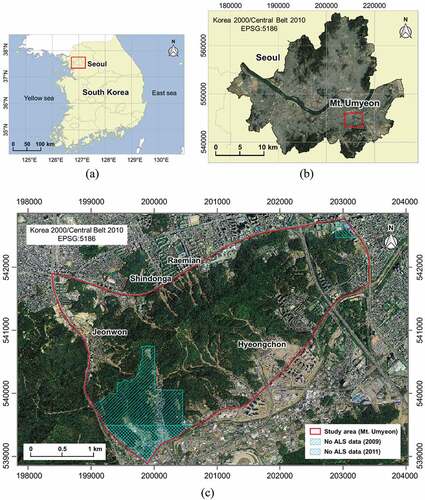
Mt. Umyeon experienced landslides due to heavy rainfalls during summer season in 2011. The rainy season, which started on 22 June 2011, lasted 26 days until July 17. A heavy rainfall, returned after 10 days from the rainy season of 26 days, led to flash flooding and subsequent landslides on Mt. Umyeon on July 27. Since Mt. Umyeon is located close to the residential area, four villages of Raemian, Shindonga, Jeonwon, and Hyeongchon were severely damaged by the rainfall-induced landslides. Fast-moving debris flows washed out narrow roads and invaded the villages, resulting in huge losses of both life and property: property damage of more than 16 billion won ($14.7 million), 18 deaths, and 21 injuries. The landslides occurred in Mt. Umyeon have been recorded as the largest natural disasters in Seoul since 2000 (Kim et al. 2017a; Seoul Metropolitan Government 2014).

2.2. ALS data

The landslide was analyzed by using two ALS datasets that were obtained between 2009 and 2011. The ALS data have been acquired through the National Geographic Information Institute (NGII) of the Ministry of Land, Infrastructure and Transport (MOLIT), Korea. The first ALS flight was conducted between August and September (the precise date is unknown), before landslide occurred. After the landslides in July 2011, additional ALS flights were carried out by NGII in August 2011. The processed ALS datasets, provided through the National Disaster Management Research Institute (NDMI), were used in this study. The basic information about ALS data is given in Table 1. However, detailed information concerning ALS dataset including strip adjustment or coordinate transformation has not been provided and both ALS datasets did not cover all the area of Mt. Umyeon. Two ALS data had the identical coordinate system of national coordinate system, Korea 2000/Central Belt 2010 (GRS80).

Table 1. Basic information about ALS data used in the study.

Category	Pre-event	Post-event
Acquisition date	15 August–16 September 2009 (exact date is unknown)	5 August 2011
Aircraft flying height	1500 m	1150 m
Flight speed	222.24 km/h	250 km/h
Laser scanner model	Leica ALS50-Ⅱ	Optech Gemini 167
Laser beam wavelength	73,500 Hz	70,000 Hz
Field of view	35°	44°
Point density	6	2.5
Coordinate system	Korea 2000/Central Belt 2010 (GRS80)

3. Methods

3.1. DEM generation from ALS data

In order to represent the bare-earth surface, several models such as regular grid, TIN, and contour line model are widely used. The regular grid model, as a kind of raster format, means the elevation of terrain surface in grid units. Amongst three different DEMs, the regular grid DEM, considered to be the simplest model, is the most efficient in terms of data processing and storage (Liu 2008). The grid DEM, on the other hand, approximates the terrain surface more than the TIN model, which is the vector model using a set of triangles. The DEM can be generated from various data such as topographic maps, remote sensing data and surveying data (Li et al. 2017). Since high-quality DEMs allow to observe terrain surface in detail, researchers have been studied on ways to generate accurate DEMs to effectively detect topographic changes (Wang et al. 2019; Daliakopoulos and Tsanis 2019; Li et al. 2017). According to the previous study showing that TIN-estimated high-resolution DEMs performed better in visual identification of landslide scarp (Chu et al. 2014), the grid DEMs of the study area were generated by two steps. First, the TIN model was constructed by using filtered point clouds. The filtered point clouds here mean terrain points, and a filtering process for accurately extracting ground points should be preceded. To extract ground points accurately, filtering method which is robust to dense vegetation and slope changes (Kim et al. 2017b) was applied. The filtering process includes two steps of extracting the lowest points and finding adjacent terrain points using the extracted lowest points. Here, this filtering method performs the axis transformation according to the slope of the study area. It is advantageous when extracting terrain information in sloped and vegetated areas. After extracting terrain points through the filtering process, TIN model was constructed. Then, the grid DEM was generated based on the elevation value from the TIN model corresponding to the center point of each grid.

3.2. Uncertainty estimation in DoD

DoD measures a vertical difference between the two DEMs on a pixel-by-pixel basis. DoD can be defined as follows:

(1) $L_{DoD}=Z_{DE{M}_2}-Z_{DE{M}_1}$(1)

where ${\mathrm{L}}_{\mathrm{D}\mathrm{o}\mathrm{D}}$ is the elevation difference between the elevation value of first DEM, ${\mathrm{Z}}_{\mathrm{D}\mathrm{E}{\mathrm{M}}_1}$ and the elevation value of second DEM, ${\mathrm{Z}}_{\mathrm{D}\mathrm{E}{\mathrm{M}}_2}$.

Since there exists uncertainty in each DEM, it is necessary to determine whether the calculated DoD is within the error budget. If it is assumed that each measurement of the DEMs is not correlated, individual errors of each DEM can be propagated as follows:

(2) ${\sigma }_{DoD}=\sqrt{{\left({\sigma }_{DE{M}_1}\right)}^2+{\left({\sigma }_{DE{M}_2}\right)}^2}$(2)

where ${\sigma }_{\mathrm{D}\mathrm{o}\mathrm{D}}$ is the propagated error in the DoD, ${\sigma }_{\mathrm{D}\mathrm{E}{\mathrm{M}}_1}$ and ${\sigma }_{\mathrm{D}\mathrm{E}{\mathrm{M}}_2}$ are the errors in the first DEM and second DEM, respectively.

DEMs generated from LiDAR measurements contain errors due to several factors. A number of studies have been conducted to estimate the LiDAR-derived DEM errors (Aguilar et al. 2010; Bilskie and Hagen 2013; Hodgson et al. 2005; Hodgson and Bresnahan 2004; Liu, Hu, and Hu. 2015; Liu et al. 2012). Major errors of the LiDAR-derived DEM, covered in previous studies, include LiDAR system error, filtering error, error due to a horizontal displacement, interpolation error, and error due to land cover types. Aguilar et al. (Aguilar et al. 2010) demonstrated that the DEM errors were related linearly with slope and inversely, nonlinearly related with ground sampling density. Hodgson and Bresnahan (Hodgson and Bresnahan 2004) found that elevation error in steep slopes (25°) was twice as large as those on a low slope (less than 4°) and the horizontal error, typically large, had more influence on the observed elevations in steep terrain. Besides the effects of surface slope on LiDAR-derived DEM, impact due to land cover types has been considered in several studies. Empirically, vegetated areas showed increased LiDAR errors compared to open terrain (Hodgson et al. 2005; Hopkinson et al. 2005; Reutebuch et al. 2003).

DEM errors were usually estimated using the law of error propagation, but some researchers estimated errors using approximation theory, arguing that each error source is not independent (Liu et al. 2012; Liu, Hu, and Hu. 2015). So far, there is no consensus on errors of LiDAR-derived DEM (Cooper et al. 2013). Hence, our study considered error components of LiDAR-derived DEM consisting of vertical LiDAR error and the error due to horizontal offset since the study area was mountainous with the high gradient. Referencing Hodgson and Bresnahan (Hodgson and Bresnahan 2004), DEM error is estimated by following Equation (3)(3) $RMS{E}_{Z_{ij}}^2=RMS{E}_{Z_{LiDAR}}^2+RMS{E}_{Horiz,Slope}^2$(3) and the following RMSE value is substituted into each DEM error.

(3) $RMS{E}_{Z_{ij}}^2=RMS{E}_{Z_{LiDAR}}^2+RMS{E}_{Horiz,Slope}^2$(3)

where $RMS{E}_{Z_{ij}}$ is a vertical error at pixel coordinate $\left(i,j\right)$ of DEM, $RMS{E}_{Z_{LiDAR}}$ is a vertical error of the LiDAR system, and $RMS{E}_{Horiz,Slope}$ is an error caused by horizontal offset expressed as the product of the horizontal offset and the tangent of slope angle.

3.3. Landslide detection

To distinguish actual surface changes, the minimum level of detection threshold (minLoD) is the most commonly adopted measure in DEM (Fuller et al. 2003). By simply setting the threshold value, the elevation changes are excluded or predicted as the real surface changes. For the sake of determining minLoD, the precision of the DEM is measured by using the classical statistical theory of errors from reference data such as field surveying data (Milan, Heritage, and Hetherington 2007). However, DoD analysis using minLoD can discard the true geomorphic changes since the errors in DEMs are not spatially uniform. Hence, the spatial structure of elevation uncertainty is fundamental for DoD analysis (Wheaton et al. 2010).

Generally, flat areas have high point density and low elevation uncertainty, but sloped areas have high surface uncertainty due to high surface roughness and low point density. If the elevation uncertainty is assumed to be spatially uniform, minLoD ignores the real change where uncertainty in elevation is low and does not provide meaningful information to distinguish the change where elevation uncertainty is high (Wheaton et al. 2010). Since the study area is highly vegetated and hilly, it can be difficult to detect changes only using minLoD. Instead of the uniform threshold, a new threshold relating the spatial distribution of elevation uncertainty needs to be considered.

(4) $newLoD=t\sqrt{{\left({\hat{\sigma }}_{DE{M}_1}\right)}^2+{\left({\hat{\sigma }}_{DE{M}_2}\right)}^2}$(4)

Equation (4)(4) $newLoD=t\sqrt{{\left({\hat{\sigma }}_{DE{M}_1}\right)}^2+{\left({\hat{\sigma }}_{DE{M}_2}\right)}^2}$(4) represents probabilistic thresholding based on a critical student’s t-value applied in previous studies (Wheaton et al. 2010; Brasington, Langham, and Rumsby 2003). In Equation (4)(4) $newLoD=t\sqrt{{\left({\hat{\sigma }}_{DE{M}_1}\right)}^2+{\left({\hat{\sigma }}_{DE{M}_2}\right)}^2}$(4) , $newLoD$ is newly calculated threshold based on the $t$ at the chosen confidence level and estimated DEM errors (${\hat{\sigma }}_{DE{M}_1}$, ${\hat{\sigma }}_{DE{M}_2}$). With a user-defined confidence interval and estimated uncertainty of DoD (RMSE calculated in Equation (3)(3) $RMS{E}_{Z_{ij}}^2=RMS{E}_{Z_{LiDAR}}^2+RMS{E}_{Horiz,Slope}^2$(3) )(3) $RMS{E}_{Z_{ij}}^2=RMS{E}_{Z_{LiDAR}}^2+RMS{E}_{Horiz,Slope}^2$(3) as an alternative to minLoD, changes can be detected conservatively.

(5) $t=\frac{Z_{DE{M}_2}-{Z_{DEM}}_1}{{\sigma }_{DoD}}$(5)

In Equation (5)(5) $t=\frac{Z_{DE{M}_2}-{Z_{DEM}}_1}{{\sigma }_{DoD}}$(5) , $Z_{DE{M}_2}-{Z_{DEM}}_1$ means the value of DoD. ${\sigma }_{DoD}$ should be calculated from the error of each DEM. The t value can be set at t ≥ 1 (1σ, confidence interval as 68%) or at t ≥ 1.96 (2σ, confidence interval as 95%) (Brasington, Langham, and Rumsby 2003; Wheaton et al. 2010). In previous studies, elevation error was considered as a single value, resulting in a uniform level of detection (LoD) (Brasington, Langham, and Rumsby 2003; Milan, Heritage, and Hetherington 2007). However, since the uniform LoD is likely to discard the true terrain changes, some studies have considered spatially distributed LoD (Milan et al. 2011; Wheaton et al. 2010; Allan et al. 2012).

After considering the spatially distributed error, further probabilistic change detection based on Bayes Theorem was implemented to rigorously detect landslide changes. Based on Bayes Theorem, the prior probability is updated using additional information to calculate a conditional probability incorporating both measures (Wheaton et al. 2010). It is calculated by the following Equation (6)(6) $P\left(E|A\right)=\frac{P\left(A|E\right)P\left(E\right)}{P\left(A\right)}$(6) .

(6) $P\left(E|A\right)=\frac{P\left(A|E\right)P\left(E\right)}{P\left(A\right)}$(6)

where $P\left(E|A\right)$ is a conditional posterior probability that the elevation difference is significant. The event A means that a change (elevation difference) occurs and the event E means that an elevation change is significant. $P\left(A|E\right)$ is a probability revealed from spatial index analysis (Wheaton et al. 2010). For computing $P\left(A|E\right)$, spatial coherence index counts which represent the tendency of changes (increase or decrease) in adjacent cells are calculated. By counting pixels whose tendency (erosion or deposition) is similar to neighboring pixels, it can be estimated whether the change has occurred in the area where significant changes occurred. Then $P\left(A|E\right)$ is calculated for each pixel by applying linear transform function within the moving window. $P\left(E\right)$ is the original a priori probability that the DoD predicted elevation change is significant and can be calculated by t-score. $P\left(A\right)$ is the conditional probability of changes of erosion or deposition, and calculated by a priori probability and spatial index probability.

4. Results and discussions

4.1. ALS-derived DEM

Figure 2(a,b) shows the raw point cloud obtained in 2009 and 2011, and Figure 2(c,d) shows the filtered points that do not contain off-terrain points, respectively. In case of ALS data of 2009, the original point cloud contained 77,841,827 points then filtered point cloud had 11,382,237 points with point density as 3.64 points/m². It could be converted to mean distance between points as 0.52 m/point. In the same way, the point cloud acquired in 2011 had 32,012,596 points before filtering, then reduced to 7,648,130 points after filtering. The mean point density was 1.98 points/m² and mean spacing was 0.71 m/point, respectively.

Figure 2. LiDAR data in the study area: (a) raw point cloud of 2009; (b) raw point cloud of 2011; (c) filtered points of 2009; (d) filtered points of 2011; (e) TIN model of 2009; (f) TIN model of 2011; (g) 1-m DEM of 2009; (f) 1-m DEM of 2011.

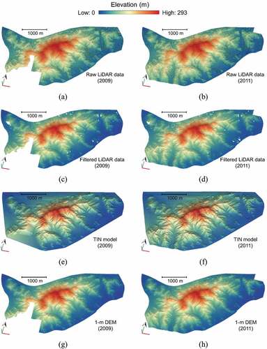
Figure 2(e,f) shows the triangular irregular network (TIN) models of each point cloud. Then, 1-m grid DEM was generated by the elevation value based on the TIN model corresponding to the center point of each grid. The 1-m resolution was determined to be suitable for gridding since the mean point spacing of each point cloud was under 1 m in the previous section. The rasterized 1-m DEMs are shown in Figure 2(g,h). The generated DEM of 2009 has a height distribution ranging from 12.23 m to 291.59 m. In the case of DEM in 2011, it has elevation values ranging from 7.66 m to 290.94 m.

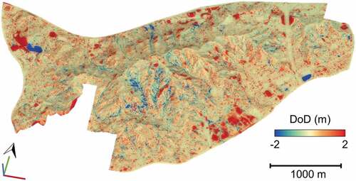
Figure 3 shows the DoD calculated by using the 1-m DEMs. The DoD ranges from – 29.58 m to 25.68 m and the average is 0.10 m. To increase the visibility, the DoD value was displayed in the range of −2 m to 2 m since the standard deviation of the DoD is 1.37 m. A red color indicates an increase in height, and blue color indicates a decrease in height. There are many areas where the elevation is decreased, and the area where the elevation is decreased is mainly distributed in high altitude areas. There are also some regions where the elevation is decreased in the low area, and those areas appear to be adjacent to the areas where the elevation increases, which seems to be due to the DEM error.

Figure 3. The spatial distribution of DoD in the study area.

4.2. Uncertainty estimation

4.2.1. Uniformly distributed uncertainty

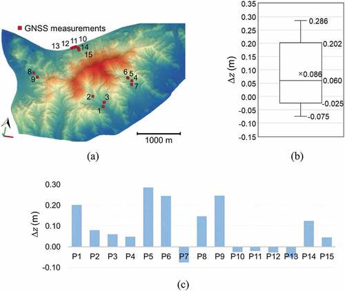
The vertical accuracy of the data was evaluated in two ways: comparison with field observations and comparison of two-point clouds. According to the investigation report for Mt. Umyeon landslide (Seoul Metropolitan Government 2014), total of 15 ground points were measured by global navigation satellite system (GNSS) surveying in the area of Mt. Umyeon after the landslide in 2011. The GNSS data were surveyed by network real-time kinematic (RTK) technique after site-calibration of the equipment. Figure 4(a) shows the location of GNSS measurements overlayed on the LiDAR data and Figure 4(b) displays the boxplot of the elevation differences between the GNSS measurements and LiDAR observations. Figure 4(c) shows differences between total of 15 GNSS heights and corresponding ALS heights. The average vertical error was 0.086 m and RMSE was calculated as 0.1425 m. Considering that typical vertical accuracy of ALS data is approximately 15 cm (Liu 2008), the calculated RMSE is a reasonable result. However, it is not wholly reliable because only 15 points were observed and only 4 points were obtained from the open terrain.

Figure 4. GNSS measurements in the study area: (a) the locations of the GNSS measurements overlayed on the point cloud; (b) boxplot of the elevation differences between GNSS measurements and LiDAR observations; (c) the elevation differences between GNSS measurements and LiDAR observations.

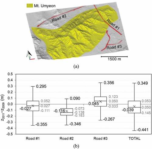
As a second way, the vertical accuracy of the data was assessed by comparing two-point clouds. The relative height accuracy is determined using extracted points in the objects that do not change over time. Three different road segments were manually extracted and their locations are displayed in Figure 5(a). The vertical differences of each road segment are plotted in Figure 5(b). The average vertical difference was −0.039 m and the root mean squared difference was 0.1762 m.

Figure 5. Vertical accuracy assessment by using stable terrain measurements: (a) location of road segments; (b) Box-and-whiskers plots representing the distribution of elevation differences of each road segment and the total.

4.2.2. Spatially distributed uncertainty

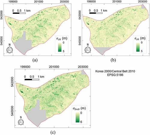
Figure 6(a,b) represents the spatial distribution of DEM error estimated by multiplying horizontal offsets and tangent of slope angles of each DEM as described in Equation (3)(3) $RMS{E}_{Z_{ij}}^2=RMS{E}_{Z_{LiDAR}}^2+RMS{E}_{Horiz,Slope}^2$(3) . The final result, DoD uncertainty calculated by using each DEM uncertainty using Equation (2)(2) ${\sigma }_{DoD}=\sqrt{{\left({\sigma }_{DE{M}_1}\right)}^2+{\left({\sigma }_{DE{M}_2}\right)}^2}$(2) , is shown in Figure 6(c). Overall, the distribution of error values showed large values. This is probably due to the poor environment at the time of acquisition of the ALS data and the failure to obtain terrain points.

Figure 6. Spatial distribution of estimated error in the study area: (a) estimated error in the DEM of 2009; (b) estimated error in the DEM of 2011; (c) estimated error of DoD.

4.3. Landslide detection

4.3.1. Change detection based on uniformly distributed uncertainty

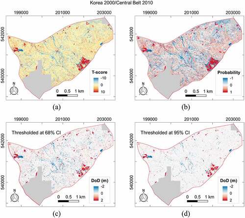
In this section, the RMSE value (0.1425 m) calculated in Section 4.2.1, was used as uniformly distributed uncertainty of the DoD. Figure 7 shows t-score distribution and the converted probability calculated by using spatially uniform DoD uncertainty. The probability was originally distributed from 0 to 1, but in Figure 7(b), the negative changes were presented with minus values to make it easier to understand; −1 means that the probability of erosion is 1, and 1 means that the probability of deposition is 1. Figure 7(c,d) shows thresholded DoDs with 68% and 95% confidence interval in the study area. Subsequently, an error-reduced DoD can be computed by eliminating changed values with probability less than the thresholds.

Figure 7. The probability calculated from DoD with uniformly distributed DEM error: (a) spatial distribution of t-score; (b) spatial distribution of the converted probability; (c) thresholded DoD with 68% confidence interval of the t-distribution; (d) thresholded DoD with 95% confidence interval of the t-distribution.

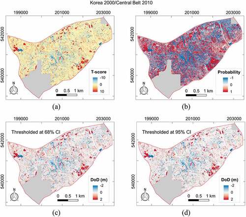
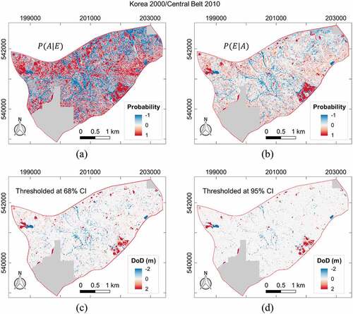
Figure 8 illustrates the probabilities updated by Bayes Theorem with uniform DEM uncertainty. In Figure 8(d), the debris flow was detected along with the stream flow of the study area with high probability. When 95% confidence interval was applied to DoD, as shown in Figure 8(d), only the changes that occurred around the stream flow were maintained noticeable, while the changes in the other regions decreased significantly. A substantial change in the positive value in the vicinity of the northern edge of the study area is actually the noise due to not-extracted-ground points in those areas.

Figure 8. The probability updated by Bayes Theorem with uniformly distributed uncertainty: (a) the probability revealed from spatial index analysis; (b) the conditional posterior probability; (c) thresholded DoD with 68% confidence interval; (d) thresholded DoD with 95% confidence interval.

4.3.2. Change detection based on spatially distributed uncertainty

However, since the uniform LoD is likely to discard the true terrain changes, some studies have considered spatially distributed LoD (Wheaton et al. 2010; Allan et al. 2012; Milan et al. 2011). Hence, spatially distributed DEM uncertainty was considered and then it was applied to calculate the probability. Figure 9(a,b) shows t-score distribution and the converted probability calculated by using spatially distributed LoD. Figure 9(c,d) show thresholded DoDs with 68% and 95% confidence interval of the t-distribution. DoD results by using a uniform LoD showed less change in comparison to the results of spatially distributed LoD. The difference was apparent when the 95% CI was applied than the 68% CI. Comparing Figures 7(d) and 9(d), more detail of changes can be identified when LoD is spatially distributed.

Figure 9. The probability calculated from DoD with spatially distributed DEM error: (a) spatial distribution of t-score; (b) spatial distribution of the converted probability; (c) thresholded DoD with 68% confidence interval of the t-distribution; (d) thresholded DoD with 95% confidence interval of the t-distribution.

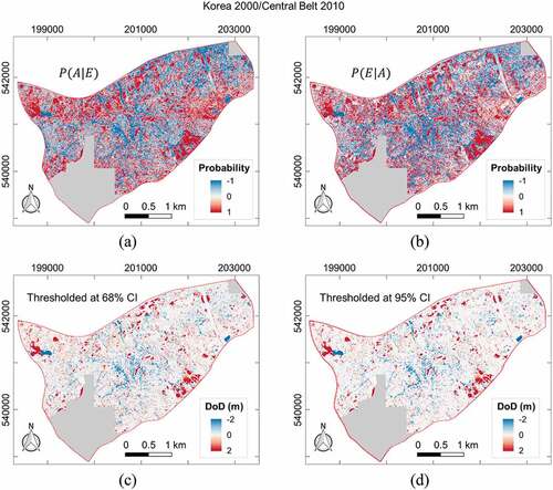
As Figure 8, the probabilities updated by Bayes Theorem with spatially distributed DEM uncertainty are shown in Figure 10. The biggest difference is that the area where change is considered significant was decreased. As a result, significant DoD shown in Figure 10(d) was also decreased. Moreover, by considering spatially distributed DEM errors, it could be identified that the false-positive detection in empty-points-region (due to filtering error) was removed effectively at a confidence interval of 95%. It shows the flow started near the top of Mt. Umyeon. In the northern part of Mt. Umyeon, the flow from the upper valley is not clearly seen, whereas in the southern part, the flow along the valley is relatively clearly seen. The significant changes were distinct in the low-lying area of northern part close to the residential area. The identified areas showed a similar pattern to the landslide distribution that can be found in the previous study (Pradhan et al. 2019).

Figure 10. The probability updated by Bayes Theorem with spatially distributed uncertainty: (a) the probability revealed from spatial index analysis; (b) the conditional posterior probability; (c) thresholded DoD with 68% confidence interval; (d) thresholded DoD with 95% confidence interval.

4.3.3. Volumetric changes

The volumetric changes were calculated as shown in Table 2 in order to quantitively analyze the changes in the study area. The volumes were calculated by using DoD with different thresholds. In “Unthresholded” case, all the DoD values were considered to compute volumetric changes. Thresholding with “Standard minLoD” used a single value to distinguish the changes. The other thresholding methods considered probability. The results of volumetric change analysis for the whole area of Mt. Umyeon showed that the deposition was larger than erosion regardless of the thresholding method, and the net volume changes were increased. This can be attributed to earthworks conducted at the construction site, which was located in the southwest of the study area.

Table 2. Volumetric changes over whole study area.

Volumetric DoD	Erosion	Deposition	Net
Unthresholded (no uncertainty)	2,214,562	3,119,195	904,633
Standard minLoD	2,087,369	2,992,826	905,457
Uniform DEM uncertainty (95% CI)	1,828,396	2,692,010	863,614
Spatially distributed DEM uncertainty (95% CI)	802,051	1,045,214	243,163
Bayesian updating with uniform DEM uncertainty (95% CI)	1,318,280	2,092,445	774,165
Bayesian updating with spatially distributed DEM uncertainty (95% CI)	705,807	933,901	228,093

(Unit: ${\mathrm{m}}^3$).

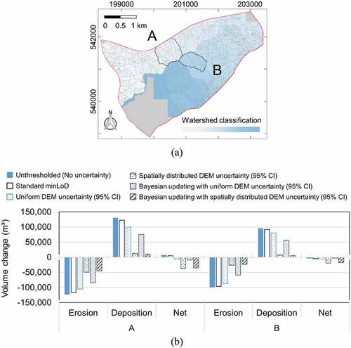
In order to grasp the volume changes caused by the landslide, it was decided to analyze the changes in a small-scale area by extracting specific watershed area. Figure 11(a) shows the selected areas A and B by delineating watersheds. The areas A and B have 485,428 m² and 313,350 m², respectively. The volumetric changes were plotted in Figure 11(b) and Table 3. In the area of B, the net DoD values are negative in any thresholding criteria, while the net DoD values in the area of A varies (positive/negative) depending on the thresholding method. This is because, considering the DEM uncertainty, the volumes became much smaller for deposition than for erosion. These differences were even more pronounced when considering spatially distributed DEM uncertainty. Moreover, this implies that the large values of net DoD loss in these areas mean that the landslide has leaked to the soils with a high probability. If DEM uncertainty was not considered and the probabilistic change detection method was not applied, the net loss would not be determined. Hence, the probabilistic landslide detection method is effective for detecting changes more reliably.

Table 3. Volumetric changes of small-scale watershed areas, A and B.

Volumetric DoD	A			B
	Erosion	Deposition	Net	Erosion	Deposition	Net
Unthresholded (no uncertainty)	123,266	130,443	7,177	100,020	95,520	−4,500
Standard minLoD	117,896	122,490	4,593	96,763	91,826	−4,937
Uniform DEM uncertainty (95% CI)	105,856	99,684	−6,172	86,648	80,444	−6,204
Spatially distributed DEM uncertainty (95% CI)	49,779	12,979	−36,800	26,634	7,450	−19,184
Bayesian updating with uniform DEM uncertainty (95% CI)	84,548	75,179	−9,369	59,328	56,202	−3,126
Bayesian updating with spatially distributed DEM uncertainty (95% CI)	45,832	10,100	−35,731	23,553	5,305	−18,248

(Unit: ${\mathrm{m}}^3$).

Figure 11. Volumetric changes in small-scale areas, A and B: (a) The location of selected areas; (b) Graph with different thresholding criteria.

5. Conclusions

The whole area of Mt. Umyeon where a landslide occurred in 2011 was hilly and covered with dense trees during summer. To reliably detect landslide by comparing two sets of DEMs derived from filtered ground points before and after the landslide, the uncertainty of DEMs was investigated. By figuring out the spatial distribution of ALS-derived DEMs uncertainty, the DoD uncertainty was estimated by the law of propagation of errors. The estimated DoD uncertainty and probabilistic analysis with Bayes’ theorem enabled to detect the landslide traces efficiently and less affected by the influence of ALS errors. When both DoD uncertainty and probabilistic analysis were considered, the difference in detected changes according to the confidence interval was obvious. The volumetric change analysis in a specific watershed of the study area showed that the changes were strictly detected in the case of deposition compared to erosion, which also affected net volume changes. When the probability with Bayesian updating and spatially distributed uncertainty was applied with 95% confidence interval, volume changes were most conservatively estimated and net changes were toward the negative direction. The results indicated that ALS-derived DEMs have a potential to detect landslides with their uncertainty estimation and a probabilistic approach, although the ALS data were acquired in hilly and densely vegetated areas. Moreover, quantifying topographic changes due to landslides with high reliability is considered to be beneficial and practically helpful for disaster recovery.

Acknowledgements

The authors are grateful to the National Disaster Management Research Institute (NDMI) in Korea for assisting this research and providing the LiDAR data. The authors would also like to thank the anonymous reviewers for their valuable comments and suggestions to improve the quality of the paper.

Disclosure statement

No potential conflict of interest was reported by the authors.

Additional information

Funding

This research was supported by a grant from the Disaster and Safety Management Institute funded by Ministry of the Interior and Safety [MOIS-DP-2015-10] and the Water Management Research Program funded by Ministry of Land, Infrastructure and Transport of Korean government [19AWMP-B121100-04].

References

- Aguilar, F. J., J. P. Mills, J. Delgado, M. A. Aguilar, J. G. Negreiros, and J. L. Pérez. 2010. “Modelling Vertical Error in LiDAR-derived Digital Elevation Models.” ISPRS Journal of Photogrammetry and Remote Sensing 65 (1): 103–110. doi:10.1016/j.isprsjprs.2009.09.003.
- Allan, J. L., M. E. Hodgson, S. Ghoshal, and M. M. Latiolais. 2012. “Geomorphic Change Detection Using Historic Maps and DEM Differencing: The Temporal Dimension of Geospatial Analysis.” Geomorphology 137 (1): 181–198. doi:10.1016/j.geomorph.2010.10.039.
- Bilskie, M. V., and S. C. Hagen. 2013. “Topographic Accuracy Assessment of Bare Earth Lidar-derived Unstructured Meshes.” Advances in Water Resources 52: 165–177. doi:10.1016/j.advwatres.2012.09.003.
- Blasone, G., M. Cavalli, L. Marchi, and F. Cazorzi. 2014. “Monitoring Sediment Source Areas in a Debris-flow Catchment Using Terrestrial Laser Scanning.” CATENA 123: 23–36. doi:10.1016/j.catena.2014.07.001.
- Bossi, G., M. Cavalli, S. Crema, S. Frigerio, B. Quan Luna, M. Mantovani, G. Marcato, L. Schenato, and A. Pasuto. 2015. “Multi-temporal LiDAR-DTMs as a Tool for Modelling a Complex Landslide: A Case Study in the Rotolon Catchment (Eastern Italian alps).” Nat. Hazards Earth Syst. Sci. 15 (4): 715–722. doi:10.5194/nhess-15-715-2015.
- Brasington, J., J. Langham, and B. Rumsby. 2003. “Methodological Sensitivity of Morphometric Estimates of Coarse Fluvial Sediment Transport.” Geomorphology 53 (3): 299–316. doi:10.1016/S0169-555X(02)00320-3.
- Bull, J. M., H. Miller, D. M. Gravley, D. Costello, D. C. H. Hikuroa, and J. K. Dix. 2010. “Assessing Debris Flows Using LIDAR Differencing: 18 May 2005 Matata Event, New Zealand.” Geomorphology 124 (1): 75–84. doi:10.1016/j.geomorph.2010.08.011.
- Burns, W. J., J. A. Coe, B. S. Kaya, and L. Ma. 2010. “Analysis of Elevation Changes Detected from Multi-Temporal LiDAR Surveys in Forested Landslide Terrain in Western Oregon.” Environmental and Engineering Geoscience 16 (4): 315–341. doi:10.2113/gseegeosci.16.4.315.
- Carlisle, B. H. 2005. “Modelling the Spatial Distribution of DEM Error.” Transactions in GIS 9 (4): 521–540. doi:10.1111/j.1467-9671.2005.00233.x.
- Cavalli, M., B. Goldin, F. Comiti, F. Brardinoni, and L. Marchi. 2017. “Assessment of Erosion and Deposition in Steep Mountain Basins by Differencing Sequential Digital Terrain Models.” Geomorphology 291: 4–16. doi:10.1016/j.geomorph.2016.04.009.
- Chen, C., X. Wang, C. Yan, B. Guo, and G. Liu. 2016. “A Total Error-based Multiquadric Method for Surface Modeling of Digital Elevation Models.” GIScience & Remote Sensing 53 (5): 578–595. doi:10.1080/15481603.2016.1172396.
- Chen, R.-F., K.-J. Chang, J. Angelier, Y.-C. Chan, B. Deffontaines, C.-T. Lee, and M.-L. Lin. 2006. “Topographical Changes Revealed by High-resolution Airborne LiDAR Data: The 1999 Tsaoling Landslide Induced by the Chi–Chi Earthquake.” Engineering Geology 88 (3): 160–172. doi:10.1016/j.enggeo.2006.09.008.
- Chu, H.-J., C.-K. Wang, M.-L. Huang, C.-C. Lee, C.-Y. Liu, and C.-C. Lin. 2014. “Effect of Point Density and Interpolation of LiDAR-derived High-resolution DEMs on Landscape Scarp Identification.” GIScience & Remote Sensing 51 (6): 731–747. doi:10.1080/15481603.2014.980086.
- Cooper, H. M., C. H. Fletcher, Q. Chen, and M. M. Barbee. 2013. “Sea-level Rise Vulnerability Mapping for Adaptation Decisions Using LiDAR DEMs.” Progress in Physical Geography: Earth and Environment 37 (6): 745–766. doi:10.1177/0309133313496835.
- Daliakopoulos, I. N., and I. K. Tsanis. 2019. “A SIFT-Based DEM Extraction Approach Using GEOEYE-1 Satellite Stereo Pairs.” Sensors (Basel, Switzerland) 19 (5): 1123. doi:10.3390/s19051123.
- Del Soldato, M., A. Riquelme, S. Bianchini, R. Tomàs, D. Di Martire, P. De Vita, S. Moretti, and D. Calcaterra. 2018. “Multisource Data Integration to Investigate One Century of Evolution for the Agnone Landslide (Molise, Southern italy).” Landslides 15 (11): 2113–2128. doi:10.1007/s10346-018-1015-z.
- DeWitt, J. D., T. A. Warner, and J. F. Conley. 2015. “Comparison of DEMS Derived from USGS DLG, SRTM, a Statewide Photogrammetry Program, ASTER GDEM and LiDAR: Implications for Change Detection.” GIScience & Remote Sensing 52 (2): 179–197. doi:10.1080/15481603.2015.1019708.
- Fernández, T., J. Pérez, C. Colomo, J. Cardenal, J. Delgado, J. Palenzuela, C. Irigaray, and J. Chacón. 2017. “Assessment of the Evolution of a Landslide Using Digital Photogrammetry and LiDAR Techniques in the Alpujarras Region (Granada, Southeastern spain).” Geosciences 7 (2): 32. doi:10.3390/geosciences7020032.
- Fey, C., M. Rutzinger, V. Wichmann, C. Prager, M. Bremer, and C. Zangerl. 2015. “Deriving 3D Displacement Vectors from Multi-temporal Airborne Laser Scanning Data for Landslide Activity Analyses.” GIScience & Remote Sensing 52 (4): 437–461. doi:10.1080/15481603.2015.1045278.
- Fowler, A., and V. Kadatskiy. 2011. “Accuracy and Error Assessment of Terrestrial, Mobile and Airborne Lidar.” Paper presented at the Proceedings of American Society of Photogrammetry and Remote Sensing Conference (ASPRP 2011), 1–5 May 2011 Milwaukee, Wisconsin.
- Fuller, I. C., A. R. G. Large, M. E. Charlton, G. L. Heritage, and D. J. Milan. 2003. “Reach‐scale Sediment Transfers: An Evaluation of Two Morphological Budgeting Approaches.” Earth Surface Processes and Landforms 28 (8): 889–903. doi:10.1002/esp.1011.
- Guzzetti, F., A. C. Mondini, M. Cardinali, F. Fiorucci, M. Santangelo, and K.-T. Chang. 2012. “Landslide Inventory Maps: New Tools for an Old Problem.” Earth-Science Reviews 112 (1): 42–66. doi:10.1016/j.earscirev.2012.02.001.
- Hodgson, M. E., J. Jensen, G. Raber, J. Tullis, B. A. Davis, G. Thompson, and K. Schuckman. 2005. “An Evaluation of Lidar-derived Elevation and Terrain Slope in Leaf-off Conditions.” Photogrammetric Engineering & Remote Sensing 71 (7): 817–823. doi:10.14358/PERS.71.7.817.
- Hodgson, M. E., and P. Bresnahan. 2004. “Accuracy of Airborne LiDAR-Derived Elevation: Empirical Assessment and Error Budget.” Photogrammetric Engineering & Remote Sensing 70 (3): 331–339. doi:10.14358/PERS.70.3.331.
- Hopkinson, C., L. E. Chasmer, I. F. Gabor Sass, M. S. Creed, W. Kalbfleisch, and P. Treitz. 2005. “Vegetation Class Dependent Errors in Lidar Ground Elevation and Canopy Height Estimates in a Boreal Wetland Environment.” Canadian Journal of Remote Sensing 31 (2): 191–206. doi:10.5589/m05-007.
- Hsieh, Y.-C., Y.-C. Chan, and J.-C. Hu. 2016. “Digital Elevation Model Differencing and Error Estimation from Multiple Sources: A Case Study from the Meiyuan Shan Landslide in Taiwan.” Remote Sensing 8 (3): 199. doi:10.3390/rs8030199.
- Hsieh, Y.-C., Y.-C. Chan, J.-C. Hu, Y.-Z. Chen, R.-F. Chen, and M.-M. Chen. 2016. “Direct Measurements of Bedrock Incision Rates on the Surface of a Large Dip-slope Landslide by Multi-Period Airborne Laser Scanning DEMs.” Remote Sensing 8 (11): 900. doi:10.3390/rs8110900.
- Kim, H., S. W. Lee, C.-Y. Yune, and G. Kim. 2014. “Volume Estimation of Small Scale Debris Flows Based on Observations of Topographic Changes Using Airborne LiDAR DEMs.” Journal of Mountain Science 11 (3): 578–591. doi:10.1007/s11629-013-2829-8.
- Kim, J., J. Park, D. K. Yoon, and G.-H. Cho. 2017a. “Amenity or Hazard? The Effects of Landslide Hazard on Property Value in Woomyeon Nature Park Area, Korea.” Landscape and Urban Planning 157: 523–531. doi:10.1016/j.landurbplan.2016.07.012.
- Kim, M.-K., S. Kim, H.-G. Sohn, N. Kim, and J.-S. Park. 2017b. “A New Recursive Filtering Method of Terrestrial Laser Scanning Data to Preserve Ground Surface Information in Steep-Slope Areas.” ISPRS International Journal of Geo-Information 6 (11): 359. doi:10.3390/ijgi6110359.
- Lague, D., N. Brodu, and J. Leroux. 2013. “Accurate 3D Comparison of Complex Topography with Terrestrial Laser Scanner: Application to the Rangitikei Canyon (N-Z).” ISPRS Journal of Photogrammetry and Remote Sensing 82: 10–26. doi:10.1016/j.isprsjprs.2013.04.009.
- Lee, C.-C., and C.-K. Wang. 2018. “Effect of Flying Altitude and Pulse Repetition Frequency on Laser Scanner Penetration Rate for Digital Elevation Model Generation in a Tropical Forest.” GIScience & Remote Sensing 55 (6): 817–838. doi:10.1080/15481603.2018.1457131.
- Li, X., H. Shen, R. Feng, J. Li, and L. Zhang. 2017. “DEM Generation from Contours and a Low-resolution DEM.” ISPRS Journal of Photogrammetry and Remote Sensing 134: 135–147. doi:10.1016/j.isprsjprs.2017.09.014.
- Liu, X. 2008. “Airborne LiDAR for DEM Generation: Some Critical Issues.” Progress in Physical Geography 32 (1): 31–49. doi:10.1177/0309133308089496.
- Liu, X., H. Hu, and P. Hu. 2015. “Accuracy Assessment of LiDAR-Derived Digital Elevation Models Based on Approximation Theory.” Remote Sensing 7 (6): 7062. doi:10.3390/rs70607062.
- Liu, X., P. Hu, H. Hu, and J. Sherba. 2012. “Approximation Theory Applied to DEM Vertical Accuracy Assessment.” Transactions in GIS 16 (3): 397–410. doi:10.1111/tgis.2012.16.issue-3.
- Milan, D. J., G. L. Heritage, and D. Hetherington. 2007. “Application of a 3D Laser Scanner in the Assessment of Erosion and Deposition Volumes and Channel Change in a Proglacial River.” Earth Surface Processes and Landforms 32 (11): 1657–1674. doi:10.1002/esp.1592.
- Milan, D. J., G. L. Heritage, R. G. L. Andrew, and I. C. Fuller. 2011. “Filtering Spatial Error from DEMs: Implications for Morphological Change Estimation.” Geomorphology 125 (1): 160–171. doi:10.1016/j.geomorph.2010.09.012.
- Mora, O. M., C. T. Lenzano, D. Grejner-Brzezinska, and J. Fayne. 2018. “Landslide Change Detection Based on Multi-Temporal Airborne LiDAR-Derived DEMs.” Geosciences 8 (1): 23. doi:10.3390/geosciences8010023.
- Picco, L., L. Mao, M. Cavalli, E. Buzzi, R. Rainato, and M. A. Lenzi. 2013. “Evaluating Short-term Morphological Changes in a Gravel-bed Braided River Using Terrestrial Laser Scanner.” Geomorphology 201: 323–334. doi:10.1016/j.geomorph.2013.07.007.
- Pike, R. J. 1988. “The Geometric Signature: Quantifying Landslide-terrain Types from Digital Elevation Models.” Mathematical Geology 20 (5): 491–511. doi:10.1007/BF00890333.
- Pradhan, A. M. S., H.-S. Kang, J.-S. Lee, and Y.-T. Kim. 2019. “An Ensemble Landslide Hazard Model Incorporating Rainfall Threshold for Mt. Umyeon, South Korea.” Bulletin of Engineering Geology and the Environment 78 (1): 131–146. doi:10.1007/s10064-017-1055-y.
- Pradhan, B. 2017b. Laser Scanning Applications in Landslide Assessment. Berlin: Springer International Publishing.
- Pradhan, B., and M. R. Mezaal. 2017a. “Optimized Rule Sets for Automatic Landslide Characteristic Detection in a Highly Vegetated Forests.” In Biswajeet Pradhan (Eds.), Laser Scanning Applications in Landslide Assessment, 51–68. New York, NY, USA: Springer.
- Reutebuch, S. E., R. J. McGaughey, H.-E. Andersen, and W. W. Carson. 2003. “Accuracy of a High-resolution Lidar Terrain Model under a Conifer Forest Canopy.” Canadian Journal of Remote Sensing 29 (5): 527–535. doi:10.5589/m03-022.
- Riquelme, A., M. Del Soldato, R. Tomás, M. Cano, L. J. Bordehore, and S. Moretti. 2019. “Digital Landform Reconstruction Using Old and Recent Open Access Digital Aerial Photos.” Geomorphology 329: 206–223. doi:10.1016/j.geomorph.2019.01.003.
- Seoul Metropolitan Government. 2014. “Investigation of the Cause of the Umyeon Nature Park Landslide”, Accessed 20 February 2019. http://www.prism.go.kr/homepage/researchCommon/downloadResearchAttachFile.do?work_key=001&file_type=CPR&seq_no=002&pdf_conv_yn=N&research_id=6110000-201400017
- Spinetti, C., M. Bisson, C. Tolomei, L. Colini, A. Galvani, M. Moro, M. Saroli, and V. Sepe. 2019. “Landslide Susceptibility Mapping by Remote Sensing and Geomorphological Data: Case Studies on the Sorrentina Peninsula (Southern italy).” GIScience & Remote Sensing 56 (6): 940–965. doi:10.1080/15481603.2019.1587891.
- Wang, S., Z. Ren, C. Wu, Q. Lei, W. Gong, Q. Ou, H. Zhang, G. Ren, and C. Li. 2019. “DEM Generation from Worldview-2 Stereo Imagery and Vertical Accuracy Assessment for Its Application in Active Tectonics.” Geomorphology 336: 107–118. doi:10.1016/j.geomorph.2019.03.016.
- Wheaton, J. M., J. Brasington, S. E. Darby, and D. A. Sear. 2010. “Accounting for Uncertainty in DEMs from Repeat Topographic Surveys: Improved Sediment Budgets.” Earth Surface Processes and Landforms 35 (2): 136–156. doi:10.1002/esp.1886.