Analysis of differences in vegetation phenology cycle of abandoned farmland, using harmonic analysis of time-series vegetation indices data: the case of Gwangyang City, South Korea

ABSTRACT

Globally, countries have experienced substantial increases in farmland abandonment. Although vegetation phenology is a key factor for the classification of land use, understanding of the phenological change of abandoned farmland is lacking. Using harmonic analysis of NDVI and NDWI extracted from Landsat imagery, this study investigates the distinctive phenological characteristics of abandoned farmland, which contrasts with that of three other agricultural types (paddy, agricultural field, orchard) in the study site of Gwangyang City in Jeollanam Province, South Korea. The results suggest that abandoned farmland has higher overall greenness coverage and overall water content in vegetation than the other uses. In terms of both indices, abandoned farmlands changed with relatively less fluctuation than those of other uses, suggesting the existence of constant and unmanaged vegetation from ecological succession, which differs from crop fields that undergo cultivation procedures. The significant harmonic components differed among agricultural types and vegetation indices. In paddy, NDVI was explained with multiple, higher-order harmonic components, while in other types only first-order components met the 5% statistical significance level. With NDWI, land types were more clearly discernible, because of the different cultivation procedures involving water: wet-field method (paddy), dryland farming (orchard, agricultural field), and no cultivation (abandoned farmland). The analysis confirms that harmonic analysis could be useful in discerning abandoned farmland among areas of active agricultural use and shows that the statistical significance of harmonic terms can be employed as indicators of different agricultural types. The observed pattern of the geographic distribution of abandoned farmland has policy implications for the promotion of sustainable reuse of marginal farmland.

KEYWORDS:

• Abandoned farmland
• vegetation phenology
• harmonic analysis
• Landsat time series

1. Introduction

Worldwide, as of 2012, 11% of land was used for agricultural production (Alexandratos and Bruinsma 2012). This proportion has been decreasing rapidly, so that some countries in the European, American, and Asian continents have experienced substantial increases in farmland abandonment, wherein production activities have ceased for several years (Alcantara et al. 2012; Keenleyside, Tucker, and Andrew 2010; Li and Xiubin 2017; Nishihara 2012). Globally, this phenomenon has been accelerating, and the total area of abandoned farmland amounted to 207 million hectares as of 1990, although it had been estimated to be a mere 15 million and 68 million hectares in 1910 and 1950, respectively (Ramankutty and Foley 1999).

The abandoned farmland has generated negative effects on rural societies ecologically and sociologically (Li and Xiubin 2017). The ecological impacts can be considered to be positive in some ways, since abandoned farmland tends to host ecological succession and become assimilated with nearby natural lands and consequently to increase biodiversity (Orłowski 2005; Plieninger et al. 2014). The revegetated lands contain more water and carbon within the soil, stabilizing the water and carbon cycles of ecosystems (Benayas et al. 2007; Lesschen et al. 2008; Li and Xiubin 2017), and the reduction of pesticide use contributes to better water quality (Lesschen et al. 2008; Stoate et al. 2001). However, negative effects are also widely known, such as ecological succession on one abandoned farmland triggering the same process on nearby cultivated lands, which is harmful to agricultural yields (Gellrich and Zimmermann 2007; Smelansky 2003; Choi et al. 2005). Also, land abandonment increases the danger of natural disasters: landslides increase on sloped farmland due to lack of maintenance (Khanal and Watanabe 2006), wildfires increase by accumulation of biomass fuel from ecological succession (Moreira and Russo 2007), and soil erosion increases in semiarid areas when the land remains bare (García-Ruiz and Lana-Renault. 2011; Li and Xiubin 2017). Also, farmland abandonment clearly generates negative impacts on rural society. In addition to the decline of food productivity (Corporation 2013), abandonment itself intensifies the rural exodus and the consequential deterioration of rural infrastructure (Li and Xiubin 2017; Pointereau 2008). The farming culture, the rural landscape, and its esthetic value are diminished as well (Benjamin, Domon, and Bouchard 2005). The loss of these unique resources turns rural areas into unattractive places, reducing the number of tourists (Benayas et al. 2007; Lasanta et al. 2017; Milenov et al. 2014; Ruskule et al. 2013).

Since the negative effects of farmland abandonment are substantial, the management of those lands has not been an easy task, due to the difficulties in detecting the sites and updating the data. To detect abandoned lands, manual surveys are necessary to investigate the fields and confirm the abandonment (Alcantara et al. 2012). For example, in Europe since 2006, Land Use/Land Cover Area Frame Survey (LUCAS) was implemented in every third year to investigate current land uses, including abandoned farmland, by field survey for physically accessible samples or photo-interpretation for non-accessible samples (Eurostat 2015; Estel et al. 2015). Despite the tremendous effort, however, LUCAS cannot be an accurate dataset, as a large portion of the abandoned farmlands was located in remote areas such as mountainous terrain (Benayas et al. 2007), while the photo-interpretation does not provide information that is as detailed as that of the field survey. In the US, the National Agricultural Statistics Services (NASS) records the location of abandoned farmlands, called Cropland Data Layer, but its accuracy varies widely by region, ranging from 42.6% for the North-west to 89.2% for East-central (Reitsma et al. 2016).

The South Korean government has tried to make a precise inventory of abandoned farmland since 1990 and has tracked abandoned land parcels every year by conducting site surveys on sampled agricultural parcels (Korea 2016). However, the survey is based on random samples, amounting to approximately 3% of the total agricultural land parcels in the country (Korea 2016). It cannot represent the comprehensive distribution of the cumulative abandoned farmlands (Corporation 2013). For the first time in 2013, the government conducted a complete survey of all land parcels in the country to detect abandoned farmland; however, such an effort could not be continued due to the extensive budget and time taken for the task (Corporation 2013).

To automate the aforementioned manual work and find the entire distribution of abandoned farmland, remote sensing techniques and machine learning have been used (Alcantara et al. 2012; Estel et al. 2015; Prishchepov et al. 2012; Yin et al. 2018; Yusoff and Muharam 2015). For agricultural land-cover classifications, studies have assessed the difference in vegetation phenology, derived from remote sensing imagery, of different types of land surface that present a different growing cycle (Pastor-Guzman, Dash, and Atkinson 2018). Often, those phenology data are used as input variables for a machine-learning algorithm such as support vector machine (SVM) and random forest to classify land cover (Alcantara et al. 2012; Conrad et al. 2011; Estel et al. 2015).

Although the vegetation phenology is a key factor for classification, understanding of the phenological change of abandoned farmland is lacking. Abandoned farmland has distinctive characteristics of change due to the ecological succession. Most of the extant studies, however, have focused on the mapping of abandoned farmland distribution using the change of reflectance bands (Alcantara et al. 2012; Baumann et al. 2011; Li and Xiubin 2017). Several studies focused on information extracted from the phenology trajectory, such as the timing, length, and integral of growing period, timing of planting and harvesting, and maximum and minimum values of specific vegetation indices, as input data for the classification (Alcantara et al. 2012; Yusoff and Muharam 2015).

Against this backdrop, we aim to investigate the distinctive phenological characteristics of abandoned farmland from the three major agricultural types in South Korea (paddy, agricultural field, orchard) by assessing seasonal changes of vegetation indices with harmonic analyses. Harmonic analysis is a kind of mathematical procedure used for analyzing a time series with a single or multiple periodic cycles (Ibrahim et al. 2018; Jakubauskas, Legates, and Kastens 2001). This method is based on an assumption that any signals can be broken down to multiple pairs of sine and cosine curves. A phenology of vegetation presents a form of cycle, due to its strong seasonality, and thus different vegetation types can be expressed with different numbers, amplitudes, and phases of sinusoid components (Ibrahim et al. 2018; Jakubauskas, Legates, and Kastens 2001). To capture the phenological characteristics of land uses and crop types, research has been conducted with harmonic analyses, and used the results to smooth and fill the gap in time series of vegetation (Roerink, Menenti, and Verhoef 2000; Xu and Shen 2013; Silveira et al. 2019), or classify land surfaces (Azzali and Menenti 2000; Canisius, Turral, and Molden 2007; Ibrahim et al. 2018; Immerzeel, Quiroz, and De Jong 2005; Jakubauskas, Legates, and Kastens 2002, 2001; Mingwei et al. 2008; Moody and Johnson 2001; Wagenseil and Samimi 2006).

However, to the best of our knowledge, no study has analyzed the phenology of abandoned farmland based on the various orders of decomposed components from the harmonic analyses. Only a few studies have looked at the seasonal change of abandoned farmland using harmonic analysis. For example, Canisius, Turral, and Molden (2007), by using the amplitude and phase of the first and second harmonic components derived from NDVI time series of Advanced Very High Resolution Radiometer (AVHRR) images, captured the temporal variability of greening process in the fallow fields of single-cropped lands.

Since the current status of abandoned farmland is diverse, and it may or may not have vegetation that is different from agricultural crops, we hypothesized that the unique characteristics of harmonic components – the sign, magnitude and the statistical significance of the coefficients – might differ from those of active agricultural land covers. Those attributes have the potential to become parameters useful for discerning the abandoned farmland. Under an assumption that the components with statistical significance would validly explain the underlying cycle, we also simulate the vegetation phenology with harmonic components of a 5% level statistical significance level.

Through this research, we expect to assess whether the phenological characteristics of abandoned farmland contrast with that of the three other agricultural types (paddy, agricultural field, orchard) and compare the trajectory of vegetation indices. Since the land surface of abandoned farmland varies from bare soil to forest (Benayas et al. 2007; Kline, Singh, and Dale 2013), our study demonstrates the phenological characteristics of abandoned farmland specifically. The revealed phenology information would provide better understanding of the current status and characteristics of abandoned farmlands, and new classification parameter for mapping the abandoned farmland for better management of the agricultural resources.

2. Materials and methodology

2.1. Study site

The study site is Gwangyang, one of the major cities in Jeollanam Province in South Korea (Figure 1). It is located between latitudes 34°53′ and 35°11′N and longitudes between 127°32′ and 127°47′E, covering 462.25 $k{m}^2$. The city is on the southern coast of South Korea; thus, its northern terrain is predominantly mountainous and the central and southern regions are relatively flat. The climate is humid subtropical, and the average temperature is about 14°C, while the maximum and minimum temperatures are 37°C in August and −10°C in January, respectively, suggesting a wide range of variability. The annual cumulative precipitation is between 1200 mm and 2000 mm, and 60% of it is concentrated during the summer season (city 2019).

Figure 1. Location of Jeollanam Province and Gwangyang City, with the boundary of Landsat tile, based on the continuous cadastral map in Jan 2018 (on the left side) and Landsat 7 band 1 image on 15 October 2000 (on the right side).

The study site, Gwangyang city, is one of the most representative among cities that have undergone a deterioration of agriculture due to rapid industrialization and have experienced the negative consequences of the abandoned farmlands (Song, Kang, and Lee 2000). Its geographic and agricultural characteristics have exacerbated the situation, as 64.8% of Gwangyang is mountainous and many agricultural fields suffered from steep slopes and low-quality infrastructures (Chae et al. 2014).

2.2. Data

2.2.1. Data collection

Our primary data is 30-m-resolution Landsat 7 ETM+ Level-2 images obtained from the United States Geological Survey (USGS). We acquired all the available 26 Tier 1 Landsat images (path/row: 115/36), covering our research site from Jan 2011 to Dec 2012, since a land parcel that remains for 2 years without agricultural activities is considered to be abandoned in South Korea (Corporation 2013). Despite the stripes caused by the Scan Line Corrector (SLC) – off issue, we used the Landsat 7 images, the only Landsat dataset over our study period 2011–2012. The stripes were treated as no values without estimating the missing values with a gap-filling method. Only the pixels labeled as “clear” from the Pixel Quality Band, generated by the CFMask (Function of Mask) algorithm, were used. Due to the lack of clear pixels at three of the obtained 26 Tier 1 Landsat images, the 23 images were finally adopted in our further analysis (Table 1). Using the “geotiffread” function programmed in MATLAB R2017b, we extracted surface reflectance by multiplying scale factor 0.0001 and the Digital Number (DN) of Landsat 7 Level-2 images. Based on the surface reflectance, we conducted further calculation of vegetation indices on Equations (1)(1) $NDVI=\frac{NIR-Red}{NIR+Red}$(1) , (2(2) $NDWI=\frac{NIR-SWIR}{NIR+SWIR}$(2) ) in the next sub-chapter.

Table 1. List of Landsat 7 images containing reference samples.

2011	2012
15 Jan	2 Jan
31 Jan	3 Feb
4 Mar	19 Feb
5 Apr	7 Apr
7 May	23 Apr
8 Jun	9 May
11 Aug	10 Jun
27 Aug	28 Jul
30 Oct	30 Sep
15 Nov	16 Oct
17 Dec	1 Nov
	19 Dec

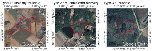
Our reference dataset is the complete survey of abandoned farmland made in 2013, from Korea Rural Community Corporation. The data is based on the photo-interpretation of surveyors. The surveyors, by visually comparing agricultural parcels in a Korea cadastral map in 2013, and orthophotos in 2010 and 2012 with a resolution of more than 0.5 m per pixel, distinguished abandoned parcels of the three categories (Figure 2): instantly reusable (type 1), reusable after recovery processes (type 2), and unusable for agriculture (type 3). The result of the complete survey is not publicly accessible, except for Gwangyang city. Among the three categories, only types 2 and 3 are available, consequently, we included those two types in our analyses. We believed that including the type 1 might make the analysis more difficult, since those instantly reusable land parcels undergo the first stage of natural succession, and would be similar to agricultural or fallow farmland in terms of vegetation phenology.

Figure 2. Google Earth high-resolution satellite images (24 October 2013) of the three categories of abandoned farmland.

2.2.2. Vegetation indices

The vegetation indices we used are NDVI (Normalized Difference Vegetation Index) and NDWI (Normalized Difference Water Index) extracted from Landsat imagery. For time-series analysis, we used both NDVI and NDWI to understand vegetation phenology. NDVI is the most often used index, quantifying the vigor of vegetation as a value between −1 and 1 (Bannari et al. 1995; Xue and Su. 2017). However, since negative NDVI value means an absence of vegetation, values above 0 are commonly used, and a value closer to 1 indicates more vigorous vegetation (Hird and McDermid 2009). NDWI is a generalized index, representing the presence of vegetation liquid water as a value between −1 and 1 (Gao 1996). Compared to NDVI, NDWI is sensitive to changes in the water content of vegetation canopy and leaf moisture. The NDWI value is negative for bare soil and dry, dead vegetation, and a value closer to 1 indicates high vegetation water content and vegetation cover (Gao 1996; Xiao et al. 2002). To calculate the vegetation indices, we used the equations as follows:

(1) $NDVI=\frac{NIR-Red}{NIR+Red}$(1)

(2) $NDWI=\frac{NIR-SWIR}{NIR+SWIR}$(2)

The spectral reflectance on the equations is based on Landsat 7 ETM+ bands. Near-infrared region (NIR) is Band 4 (Near Infrared, 0.772–0.898 µm), red region (Red) is Band 3 (Red, 0.631–0.692 µm), and short-wavelength infrared region (SWIR) is Band 5 (Short Wavelength Infrared, 1.547–1.749 µm).

2.2.3. Sampling of abandoned farmland, paddies, agricultural fields, and orchards

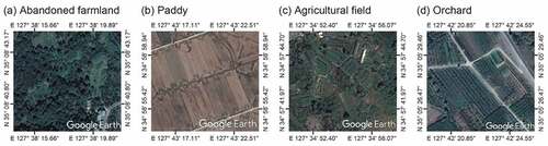
The site contains 52,365 paddy parcels, 28,867 agricultural field parcels, and 116 orchard parcels, according to the continuous cadastral map published in Jan 2018 by the Ministry of Land Infrastructure and Transport of South Korea. Paddy means the cropland where crops are cultivated with a distinctive water usage. The lower part of the crops is submerged in water for at least several months before harvests. Rice, lotus, and water parsley are some of the examples produced in paddy. Agricultural field means the cropland where grain and horticultural crops are growing, without the water-related process of paddy. Orchard means the croplands of fruit trees. Among these, we selected 400 random samples for each agricultural land use – paddy, agricultural field, and orchard – a total of 1200 parcels, and cross-checked the validity of the sample using Google Earth’s high-resolution images from 2011 to 2012, to see whether land was actually used for the designated uses. Some of the agricultural fields were found to be in use as orchards; thus, we corrected those discrepancies and selected 400 orchard samples from there.

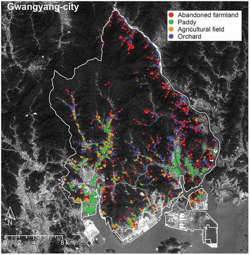
For the abandoned farmland samples, we used the result of the complete survey of abandoned farmland in 2013, provided by the agricultural support division of Gwangyang. We randomly selected 400 parcels from the inventory and used the abandoned farmland categorized in type 2 and 3 only due to the aforementioned reason. For the selected 400 parcels, we checked their abandoned status by comparison with high-resolution images from Google Earth taken from 2011 to 2012. Figure 3 depicts the distribution of the samples.

Figure 3. Location of reference samples in Gwangyang City, based on Landsat 7 band 1 image on 15 October 2000.

The sampled paddies are located mostly in the southern part of the city, where the dominant terrain is flat near the shoreline, or in the central area, on the plain near streams. The prevalent farming method is wet-field cultivation, requiring the transplant of rice seedlings to paddies in May. For this reason, the presence of vegetation begins to be observed in paddies in that season. Rice is grown during the summer season and harvested between September and October (Administration, 2019). Compared to paddies, the size of agricultural fields is relatively small and sparsely distributed, and most of the samples are located at the edge of mountainous areas around the central and southern parts of the city. In those parcels, frequent planting and harvesting of crops occurs in the order bean, pepper, cabbage, perilla, and sesame, thus the cultivation pattern of those agricultural fields becomes unclear (Chae et al. 2014; Gwangyang 2019). Most of the orchard samples are located in the central part and the northern part. The leaves begin growth in March and fall in November, but the harvest periods for various fruits are different; for example, June for plum and October for persimmon (Administration, 2019).

The abandoned farmland samples are most widely distributed in mountainous areas throughout the city. Unlike other types of agricultural land uses, abandoned parcels are on steep slopes and high elevation. When agricultural land is abandoned, first weeds invade the land, and then shrubs and trees dominate in succession. Consequently, the presence of vegetation is consistent in abandoned land parcels throughout the year (Benjamin, Domon, and Bouchard 2005; Yusoff and Muharam 2015). Figure 4 depicts the growth period of crops within the study site, and Figure 5 shows the appearance of each agricultural type.

Figure 4. Crop calendar in Gwangyang City.

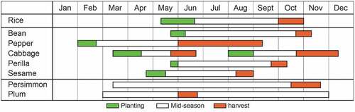
Figure 5. Google Earth high-resolution satellite images (24 October 2013) of reference samples for four agricultural types.

2.3. Harmonic analysis

Harmonic analysis decomposes a periodic function into a series of basic sinusoids, a set of sine or cosine terms having unique coefficients and intercept (Jakubauskas, Legates, and Kastens 2001; Moody and Johnson 2001; Wagenseil and Samimi 2006). The function$f\left(t\right)$ represents a general cyclic model with harmonic components:

(3) $f\left(t\right)=a_0+\sum _{n=1}^{L/2}(a_{n}cos\frac{2\pi nt}{L}+b_{n}sin\frac{2\pi nt}{L})$(3)

L is the length of the phenology period, having the value 24, the time interval at bi-monthly scale in a year; $a_n$ and $b_n$ denote the coefficients of the sine and cosine components of the $n$th harmonic term, respectively. Higher-order harmonic components have a higher frequency. Among the available frequencies, from 1/L to ½, we limited the six lowest frequencies for the initial modeling, as they explain the overall cycle with statistical significance (Ibrahim et al. 2018; Metcalfe and Cowpertwait 2009; Moody and Johnson 2001). Consequently, the original signal was decomposed into six sine and six cosine curves. Normally the lower frequency components are known to represent the seasonal fluctuations, while higher frequency components does for temporal anomalies of vegetation conditions induced by floods or droughts (Moody and Johnson 2001). To the best of our knowledge, other harmonic studies used a small, fixed number of harmonic components without considering their statistical significance (Ibrahim et al. 2018). Generally, the first and second harmonic components (Canisius, Turral, and Molden 2007; Ibrahim et al. 2018; Immerzeel, Quiroz, and De Jong 2005; Moody and Johnson 2001) are used for the analysis, as those harmonic terms followed the annual phenology of vegetation in the temperate climate where single or double cropping is dominant (Devendra and Thomas 2002). Sometimes the third harmonic is used for the analysis to distinguish specific vegetation such as winter wheat (Mingwei et al. 2008) or shrub in savannah (Wagenseil and Samimi 2006). The harmonic components over the third order were frequently ignored and considered as noise (Wagenseil and Samimi 2006).

However, since there is a possibility that the higher-order harmonic components could capture the truthful and distinctive features of plant-growing trajectory, we used those components that are statistically significant in explaining the phenology of the vegetation indices among the 12 decomposed sinusoids curves. General interpretations of a regression function apply here, in that only statistically significant independent variables have an explanatory power for the dependent variable. The independent variables are harmonic components and the dependent variable is the vegetation indices. In other words, by combining the statistically significant harmonic terms, we could explain the vegetation phenology represented with vegetation indices. Thus, we analyzed not only the coefficients of the harmonic components but also the pattern of statistically significant harmonic terms to distinguish abandoned farmland from other land uses.

3. Results

3.1. Time series of NDVI and NDWI by agricultural type

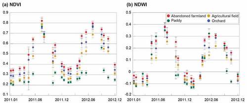
The cycles of NDVI and NDWI differ by the agricultural land type (Figure 6). As presented in Figure 6(a), the NDVI value is highest in abandoned farmland for most of the periods, followed by orchard, agricultural field, and paddy. All curves are bell-shaped, peak in July, and bottom out between January and February. Compared to other uses, the NDVI curve for paddy increases sharply after June and then decreases after September, indicating the seedling stage and harvest of the rice plants, respectively. The NDVI curves of paddy in the late spring, fall, and winter also apparently differ from those of the other agricultural land uses. In those seasons, greenness from vegetation is not present in paddies, while in the rest of the use types, vegetation remains due to late harvesting or no harvesting processes.

Figure 6(b) presents the cycles of NDWI by agricultural land-use type. The trajectory is apparently similar to that of NDVI, since both indices are related to vegetation growth (Delbart et al. 2005). All curves peak in July and bottom out between December and February. The NDWI values, however, are quite different from the NDVI values. In June, the NDWI value is highest in paddy, while the equivalent NDVI value is the lowest among all land types, suggesting the effect of wet-field cultivation on paddy; paddies are filled with water for transplanting at these seasons. On the other hand, the NDWI value of agricultural field and orchard types is lowest between May and September due to the harvest of crops such as pepper from early June until early September, spring cabbage in late May and middle June, and plum in June.

Figure 6. Average vegetation indices with their 95% confidence intervals, showing annual change over 2 years, for all 400 reference samples by agricultural type.

3.2. Harmonic analysis of NDVI and NDWI by agricultural type

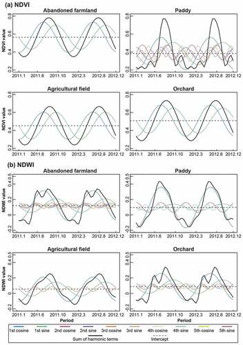
The harmonic components of NDVI and NDWI also differ by the agricultural land type. Table 2 presents the results of harmonic analysis, and Figure 7 presents the fitted curves with the subject harmonic models. From Table 2, it can be learned that statistically significant harmonic components differ by agricultural type and vegetation index.

Table 2. The set of statistically significant harmonic components for each agricultural type and for NDVI and NDWI.

(1)NDVI	Abandoned farmland	Paddy	Agricultural field	Orchard
Intercept	0.5588*** (0.0177)	0.3878*** (0.0069)	0.4545*** (0.0134)	0.5085*** (0.0137)
1st cos	−0.1784*** (0.0366)	−0.1769*** (0.0142)	−0.1555*** (0.0279)	−0.1703*** (0.0284)
1st sin	−0.1386*** (0.0226)	−0.1217*** (0.0088)	−0.1437*** (0.0172)	−0.1376*** (0.0175)
2nd cos	-	0.0629*** (0.0113)	-	-
2nd sin	-	0.0927*** (0.0100)	-	-
3rd cos	-	-	-	-
3rd sin	-	−0.0858*** (0.0100)	-	-
4th cos	-	-	-	-
4th sin	-	-	-	-
5th cos	-	−0.0383* (0.0126)	-	-
5th sin	-	-	-	-
6th cos	-	-	-	-
6th sin	-	-		-
(2)NDWI
Intercept	0.1214*** (0.0053)	0.0978*** (0.0129)	0.0554*** (0.0079)	0.0866*** (0.0063)
1st cos	−0.1953*** (0.0100)	−0.2649*** (0.0268)	−0.1569*** (0.0153)	−0.1734*** (0.0131)
1st sin	−0.0896*** (0.0062)	−0.0438* (0.0165)	−0.0915*** (0.0094)	−0.0889*** (0.0081)
2nd cos	-	0.0648** (0.0212)	-	-
2nd sin	−0.0287** (0.0070)	-	-	-
3rd cos	0.0378*** (0.0074)	-	0.0333* (0.0113)	0.0395** (0.0097)
3rd sin	0.0233** (0.0071)	-	-	-
4th cos	−0.0364** (0.0096)	-	-	−0.0408** (0.0125)
4th sin	0.0271** (0.0063)	−0.0408* (0.0169)	-	0.0308** (0.0082)
5th cos	-	-	-	-
5th sin	−0.0196* (0.0070)	-	-	−0.0265* (0.0091)
6th cos	-	-	-	-
6th sin	-	-	-	-

Standard errors in parentheses; ***p < 0.001, **p < 0.01, *p < 0.05

For NDVI of three agricultural types – abandoned farmland, agricultural field, and orchard – only intercepts are useful in distinguishing the phenology trajectory among different use types. Although the first pair of the cosine and sine elements explains the NDVI at a 1% statistical significance level, most of those values are statistically indiscernible among others. The size of the coefficient ranges from −0.1784 to −0.1555 for cosine and from −0.1437 to −0.1217 for sine, which is within the range of the 95% confidence interval (−0.2047 to −0.1491 for cosine, −0.1389 to −0.1045 for sine). The intercepts, which represents the average vegetation indices of each agricultural type (Jakubauskas, Legates, and Kastens 2001), mostly differ among others in statistically significant level; they are 0.5588 (95% confidence interval; 0.5241–0.5935) in abandoned farmland, 0.5085 (95% confidence interval; 0.4816–0.5354) in orchard, 0.4545 (95% confidence interval; 0.4282–0.4808) in agricultural field, and 0.3878 (95% confidence interval; 0.3743–0.4013) in paddy. Even though the 95% confidence intervals between abandoned farmland and orchard are partly overlapped, the results suggest that the average greenness of the abandoned farmland is the highest, due to the active natural succession of trees and shrubs. On the other hand, the paddy has the largest number of significant components; cosine and sine in the first and second term, sine in the third term, and cosine in the fifth term explain the NDVI at a 5% statistical significance level. Among the components, the first terms describe most of the phenology, since the coefficients are the largest; −0.1769 for cosine and −0.1217 for sine.

Compared with the NDVI curves, the differences among the fitted NDWI curves are much more discernible for all of four agricultural types. The number of statistically significant components is eight for abandoned farmland (1st cosine and sine, 2nd sine, 3rd cosine and sine, 4th cosine and sine, 5th sine), six for orchard (1st cosine and sine, 3rd cosine, 4th cosine and sine, 5th sine), four for paddy (1st cosine and sine, 2nd cosine, 4th sine), and three for agricultural field (1st cosine and sine, 3rd cosine). As seen in the NDVI, the NDWI curves for paddy are the most distinctive relative to other groups.

Also, the magnitude and the sign of the coefficients of sine and cosine terms vary highly by type at a 5% statistical significance level. The first-order cosine and sine term are statistically significant in all agricultural types, and the first-order cosine term explains most of the phenology, as shown by its having the average coefficient of the greatest magnitude (−0.1976). All these differences could have been generated from the different cultivation procedures, because paddies are filled with water for most of the growing season, while other agricultural land is dry, causing different trajectories of water contents. The intercepts differ among abandoned farmland, agricultural field and orchard in statistically significant level, as the values are 0.1214 (95% confidence interval; 0.1110–0.1318) in abandoned farmland, 0.0554 (95% confidence interval; 0.0399–0.0709) in agricultural field and 0.0866 (95% confidence interval; 0.0743–0.0989) in orchard. On the other hand, the value in paddy is 0.0978 (95% confidence interval; 0.0725–0.1231), overlapping with the value of abandoned farmland and agricultural field.

Figure 7(a) depicts the phenology of NDVI by the agricultural type, using the fitted model described in Table 2. As explained above, the NDVI cycle of the abandoned farmland, agricultural field, and orchard are explained by a single pair of the harmonic components; thus, they all appear as smooth, bell-shaped curves. The intercepts, which mean average annual NDVI value, differ in decreasing order: abandoned farmland (0.5588), orchard (0.5085), and agricultural field (0.4545). On the other hand, since the phenology of paddy NDVI is explained with multiple pairs of harmonic components, the curve has more fluctuations, explaining crop stages of rice such as transplanting in late May and harvesting in late September.

Figure 7(b) depicts the phenology of NDWI by the agricultural type, using the fitted model described in Table 2. Unlike the NDVI curves, each type displays a distinctive trajectory, although those of the abandoned farmland and orchard are pretty similar. In abandoned farmland and orchard, the curve has two peaks in May and July. This might suggest that the phenology is similar on both land types, because the dominant vegetation is tree. However, the annual NDWI values differ; it is the highest in abandoned farmland (0.1214), while being relatively low in orchard (0.0866). This difference may imply a natural succession is occurring in abandoned farmland. Paddy has one peak with small fluctuation after harvest. Agricultural field also has one peak in July, but its shape is smoother and the maximum value is smallest.

Figure 7. Curves of statistically significant harmonic terms and the composite curve for each agricultural type.

4. Discussion

4.1. Analyzing phenology of abandoned farmland using harmonic analysis

We analyzed the phenology of abandoned farmland using harmonic analysis, and compared them to those of the three types of active croplands. Primary findings are that abandoned farmland generally has higher overall water content in vegetation – higher average NDWI, and higher overall greenness coverage – higher average NDVI – than the rest of the land types based on the intercept with 95% confidence interval. In terms of both indices, abandoned farmlands experienced relatively less fluctuation than paddy and orchard, suggesting the existence of constant and unmanaged vegetation from ecological succession (Alcantara et al. 2012; Benjamin, Domon, and Bouchard 2005; Choi et al. 2005).

The statistically significant harmonic components differed by agricultural type and vegetation index. For paddy, NDVI was explained with multiple, higher-order harmonic components, while for other land types the index was explained with only first-order cosine and sine terms at a 5% statistical significance level. With NDWI, land types were more distinguishable by agricultural type, because of the dominant vegetation: tree (abandoned farmland and orchard), rice (paddy), and mixed crops (agricultural field) had relatively sharp difference in water contents. For both of the harmonic components of NDVI and NDWI, the first pair of the cosine and sine elements always had explanatory power at a 5% statistical significance level, depicting the dominant annual cycle of the greenness and water content of crops and/or other natural vegetation on the land surface. Other pairs of harmonic components express the deviation from the main cycle, presenting the specific characteristics of cultivation and maintenance procedures.

This study confirms that harmonic analysis could be a useful tool to discern abandoned farmland among areas of active agricultural use. First, the majority of the extant studies used only the first and second harmonic terms for the analysis, in the belief that those describe a large part of the cyclic trajectory of vegetation indices (Immerzeel, Quiroz, and De Jong 2005; Wagenseil and Samimi 2006). The number and orders of statistically significant harmonic components, however, could be another indicator of different agricultural use types, since they also differ by vegetation characteristics as our analytical results showed. This result corresponds to the research of Mingwei et al. (2008), as the set of amplitude and phase of harmonic terms were different by crops. The first and second harmonic terms were used as classification parameters to distinguish spring maize and cotton; first, second, and third harmonic terms were used to distinguish winter wheat-maize and winter wheat cotton. Also, the sign and magnitude of the coefficients of harmonic components differ by the agricultural types including the abandoned farmland. These characteristics also can be used as a set of input data for the future classification, as an alternative to the conventional phenology metrics.

4.2. Phenological characteristics of abandoned farmland

This study confirmed the common phenological characteristics of abandoned farmland. As revealed in the previous researches (Alcantara et al., Esetl et al., Yusoff and Muharam), NDVI of abandoned farmlands is mostly higher than that of croplands. Also, the NDVI curve of abandoned farmland was smooth and bell-shaped while that of active agricultural land was an irregularly shaped with one or more narrow peaks due to the human interventions. Our analytical results reflect the results of the previous studies. The NDVI value of abandoned farmland of the study site was also higher than that of other cropland, and the shape of the NDVI curve differs from that of other cropland with the aforementioned features. While the equivalent analysis of NDWI was rare previously, our analytical results on NDWI provide valuable information. Unlike that of the NDVI, the NDWI curves of paddy and agricultural field were smoother than that of abandoned farmland, due to the constant presence of water during the growing season.

Also, this study confirmed that usefulness of using remote sensing images to analyze abandoned farmland. As the research of Zhang et al. (2017) estimated the crop map of North Korea where ground truth data is limited based on phenology features of each crop type, the phenology information is a useful indicator to differentiate abandoned farmland from other land uses since many abandoned farmlands were located in remote areas which are difficult to visit (Benayas et al. 2007).

This study demonstrates the possibility of using diversified vegetation indices for the purpose of classification. Since most of the extant research has used NDVI for the analysis (Alcantara et al. 2012; Estel et al. 2015; Smaliychuk et al. 2016; Yusoff and Muharam 2015), several disadvantages of using NDVI have been identified. NDVI is used limitedly for quantifying the vigor of green vegetation, and sensitively affected by soil brightness, soil color, and atmosphere (Bannari et al. 1995; Xue and Su. 2017). Depending on the local context, such as a case in which wet- and dry-field farming fields are intermixed, the NDWI is a more appropriate index to discern agricultural use types. Although not addressed in this study, the Soil-Adjusted Vegetation Index (SAVI) or Redness Index (RI) can be better indices for an area where root crops are dominant with exposed soil cover on the cropland (Bannari et al. 1995). For an area with heavy snow, the Normalized Difference Snow Index (NDSI) may have more potential to capture the vegetation characteristics (Delbart et al. 2005; Vescovo and Gianelle 2008).

5. Conclusion

In this study, we investigated the distinctive phenological characteristics of abandoned farmland – which differs from that of the other three agricultural types, using harmonic analysis of the two vegetation indices, NDVI and NDWI. Unlike other studies, our study began with a search for the statistically significant harmonic components explaining the cycle of vegetation and vegetation liquid water, to identify characteristics of the phenology of abandoned farmland. The results successfully showed that the signs, magnitudes and statistical significances of harmonic terms could discern the phenological characteristics of abandoned farmland from other croplands. Also, the results confirmed that not only NDVI but other vegetation index such as NDWI is a useful indicator to discern abandoned farmlands from other types of agricultural croplands. Our new approach could provide a better understanding of the phenology of abandoned farmland. Although classification was beyond the scope of this study, the results of it suggest classification parameters to increase the accuracy in the mapping of abandoned farmlands. Classification research might be benefited by the current study.

The findings of this study have policy implications. Farmland abandonments tend to occur on higher and steeper terrain with poor-quality infrastructure (Baumann et al. 2011; Kuemmerle et al. 2008; Melendez-Pastor et al. 2014). The Japanese government has implemented a policy to subsidize such regions since 2000, which successfully reduced the rate of farmland abandonment (Li and Xiubin 2017). However, despite sharing a similar context with Japan, subsidy policies in South Korea often neglected the fact that topography conditions and quality of infrastructure are closely related to farmland abandonment. Instead, the government concentrated on rice paddy, where the abandonment rate is relatively low, and used 68% of the budget for support by exempting purchases of agricultural equipment and fuel from taxation (Park et al. 2014). Even though the lack of infrastructure has exacerbated farmland abandonment (Corporation 2013; Jing’an, Zhang, and Li 2015), the government’s efforts have not been enough to improve farming infrastructure for marginal land; only 15% of agricultural fields are included in the improvement plan, and most of the existing plans have focused on simple maintenance rather than construction of new infrastructure (Chae et al. 2014; Park et al. 2014). To prevent further farmland abandonment, governments should enlarge policies that directly improve the quality of rural infrastructure, by constructing more roads, reservoirs, and other infrastructure (Chae et al. 2014), and they also need to set a priority on the marginal land with poor cultivation conditions.

In addition, the reuse strategy for currently abandoned farmland needs to be considered. In the case of Korea or countries in a similar situation, the majority of abandoned farmland exists in areas where the quality of farming conditions is poor (Choi et al. 2005; Melendez-Pastor et al. 2014), and reusing the abandoned farmland for agricultural purposes is not often practical in most instances. On the other hand, abandoned farmland tends to have a good quality of natural resources, due to the ecological succession (Orłowski 2005; Plieninger et al. 2014). This implies that afforestation on abandoned farmland might be relatively easy and that those sites might be utilized as natural amenities for local people and as habitat for wildlife (Ruskule et al. 2013). Governments should consider the site conditions and context to promote sustainable reuse of abandoned farmlands (Meyfroidt et al. 2016).

Disclosure statement

No potential conflict of interest was reported by the authors.

Correction Statement

This article has been republished with minor changes. These changes do not impact the academic content of the article.

Additional information

Funding

This research was supported by Creative-Pioneering Researchers Program through Seoul National University (SNU) under the grant number [No. 500-20170162]; and the Ministry of Education of the Republic of Korea and the National Research Foundation of Korea under Grant number [NRF-2017S1A3A2066771].

References

- Administration, Rural Development. 2019. “Crop Calendar in South Korea.” Rural Development Administration. Accessed 21 February. http://www.nongsaro.go.kr/portal/ps/psb/psbl/workScheduleLst.ps?menuId=PS00087
- Alcantara, C., T. Kuemmerle, A. V. Prishchepov, and V. C. Radeloff. 2012. “Mapping Abandoned Agriculture with Multi-temporal MODIS Satellite Data.” Remote Sensing of Environment 124: 334–347.
- Alexandratos, N., and J. Bruinsma. 2012. “World Agriculture Towards 2030/2050: The 2012 Revision.” ESA Working paper FAO. Rome.
- Azzali, S., and M. Menenti. 2000. “Mapping Vegetation-soil-climate Complexes in Southern Africa Using Temporal Fourier Analysis of NOAA-AVHRR NDVI Data.” International Journal of Remote Sensing 21 (5): 973–996. doi:10.1080/014311600210380.
- Bannari, A., D. Morin, F. Bonn, and A. R. Huete. 1995. “A Review of Vegetation Indices.” Remote Sensing Reviews 13 (1–2): 95–120. doi:10.1080/02757259509532298.
- Baumann, M., T. Kuemmerle, M. Elbakidze, M. Ozdogan, V. C. Radeloff, N. S. Keuler, A. V. Prishchepov, I. Kruhlov, and P. Hostert. 2011. “Patterns and Drivers of Post-socialist Farmland Abandonment in Western Ukraine.” Land Use Policy 28 (3): 552–562.
- Benayas, J. M., A. Martins, J. M. Nicolau, and J. J. Schulz. 2007. “Abandonment of Agricultural Land: An Overview of Drivers and Consequences.” CAB Reviews: Perspectives in Agriculture, Veterinary Science, Nutrition Natural Resources 2 (57): 1–14.
- Benjamin, K., G. Domon, and A. Bouchard. 2005. “Vegetation Composition and Succession of Abandoned Farmland: Effects of Ecological, Historical and Spatial Factors.” Landscape Ecology 20 (6): 627–647. doi:10.1007/s10980-005-0068-2.
- Canisius, F., H. Turral, and D. Molden. 2007. “Fourier Analysis of Historical NOAA Time Series Data to Estimate Bimodal Agriculture.” International Journal of Remote Sensing 28 (24): 5503–5522. doi:10.1080/01431160601086043.
- Chae, G., H. Kim, Y. Lee, G. Kim, S. Kook, and H. Mun. 2014. “Dispute and Guideline for Field Agriculture.” Korea Rural Economic Institute Agriculture Policy Focus 1–20.
- Choi, H., D. Ji, S. Choi, and S. Kim. 2005. “Institutional Improvements for the Utilization and Management of Idle Agricultural Land.” Korea Research Institute for Human Settlements.
- City, Gwangyang. 2019. “Natural Environment of Gwangyang.” Accessed 21 February. http://www.gwangyang.go.kr/index.gwangyang?menuCd=DOM_000000106001004000
- Conrad, C., R. R. Colditz, S. Dech, D. Klein, and P. L. G. Vlek. 2011. “Temporal Segmentation of MODIS Time Series for Improving Crop Classification in Central Asian Irrigation Systems.” International Journal of Remote Sensing 32 (23): 8763–8778. doi:10.1080/01431161.2010.550647.
- Corporation, Korea Rural Community. 2013. “Study on the Plan to Make High-income Agricultural Infrastructure Utilizing Idle Farmland: Centering on Business Model of utilizing idle farmland.” In Korea Rural Community Corporation, edited by J. Park. Korea Rural Community Corporation.
- Delbart, N., L. Kergoat, T. Le Toan, J. Lhermitte, and G. Picard. 2005. “Determination of Phenological Dates in Boreal Regions Using Normalized Difference Water Index.” Remote Sensing of Environment 97 (1): 26–38. doi:10.1016/j.rse.2005.03.011.
- Devendra, C., and D. Thomas. 2002. “Smallholder Farming Systems in Asia.” Agricultural Systems 71 (1–2): 17–25. doi:10.1016/S0308-521X(01)00033-6.
- Estel, S., T. Kuemmerle, C. Alcántara, C. Levers, A. Prishchepov, and P. Hostert. 2015. “Mapping Farmland Abandonment and Recultivation across Europe Using MODIS NDVI Time Series.” Remote Sensing of Environment 163: 312–325. doi:10.1016/j.rse.2015.03.028.
- Eurostat. 2015. LUCAS 2015 (Land Use/Cover Area Frame Survey). In, edited by Eurostat. Eurostat.
- Gao, B. C. 1996. “NDWI—A Normalized Difference Water Index for Remote Sensing of Vegetation Liquid water from Space.” Remote Sensing of Environment 58 (3): 257–266. doi:10.1016/S0034-4257(96)00067-3.
- García-Ruiz, J. M., and N. Lana-Renault. 2011. “Hydrological and Erosive Consequences of Farmland Abandonment in Europe, with Special Reference to the Mediterranean region–A Review.” Agriculture, Ecosystems Environment 140 (3–4): 317–338. doi:10.1016/j.agee.2011.01.003.
- Gellrich, M., and N. E. Zimmermann. 2007. “Investigating the Regional-scale Pattern of Agricultural Land Abandonment in the Swiss Mountains: A Spatial Statistical Modelling Approach.” Landscape Urban Planning 79 (1): 65–76. doi:10.1016/j.landurbplan.2006.03.004.
- Gwangyang, Agricultural Technology Center in. 2019. “Cultivation Status in Gwangyang.” Accessed 21 February. http://www.gwangyang.go.kr/jares/index.gwangyang?menuCd=DOM_000000309002000000
- Hird, J. N., and J. McDermid. 2009. “Noise Reduction of NDVI Time Series: An Empirical Comparison of Selected Techniques.” Remote Sensing of Environment 113 (1): 248–258. doi:10.1016/j.rse.2008.09.003.
- Ibrahim, S., H. Balzter, K. Tansey, N. Tsutsumida, and R. Mathieu. 2018. “Estimating Fractional Cover of Plant Functional Types in African Savannah from Harmonic Analysis of MODIS Time-series Data.” International Journal of Remote Sensing 39 (9): 2718–2745. doi:10.1080/01431161.2018.1430914.
- Immerzeel, W. W., R. A. Quiroz, and S. M. De Jong. 2005. “Understanding Precipitation Patterns and Land Use Interaction in Tibet Using Harmonic Analysis of SPOT VGT‐S10 NDVI Time Series.” International Journal of Remote Sensing 26 (11): 2281–2296. doi:10.1080/01431160512331326611.
- Jakubauskas, M. E., D. R. Legates, and J. H. Kastens. 2001. “Harmonic Analysis of Time-series AVHRR NDVI Data.” Photogrammetric Engineering Remote Sensing 67 (4): 461–470.
- Jakubauskas, M. E., D. R. Legates, and J. H. Kastens. 2002. “Crop Identification Using Harmonic Analysis of Time-series AVHRR NDVI Data.” Computers Electronics in Agriculture 37 (1–3): 127–139. doi:10.1016/S0168-1699(02)00116-3.
- Jing’an, S., S. Zhang, and X. Li. 2015. “Farmland Marginalization in the Mountainous Areas: Characteristics, Influencing Factors and Policy Implications.” Journal of Geographical Sciences 25 (6): 701–722. doi:10.1007/s11442-015-1197-4.
- Keenleyside, C., G. Tucker, and M. Andrew. 2010. Farmland Abandonment in the EU: An Assessment of Trends and Prospects. Institute for European Environmental Policy, London.
- Khanal, N. R., and T. Watanabe. 2006. “Abandonment of Agricultural Land and Its Consequences.” Mountain Research and Development 26 (1): 32–41. doi:10.1659/0276-4741(2006)026[0032:AOALAI]2.0.CO;2.
- Kline, K. L., N. Singh, and V. H. Dale. 2013. “Cultivated Hay and Fallow/idle Cropland Confound Analysis of Grassland Conversion in the Western Corn Belt.” Proceedings of the National Academy of Sciences 110 (31): E2863–E. doi:10.1073/pnas.1306646110.
- Korea, S. 2016. Statistics of Agricultural Area in 2015. Statistics Korea. South Korea.
- Kuemmerle, T., P. Hostert, V. C. Radeloff, S. van der Linden, K. Perzanowski, and I. Kruhlov. 2008. “Cross-border Comparison of Post-socialist Farmland Abandonment in the Carpathians.” Ecosystems 11 (4): 614. doi:10.1007/s10021-008-9146-z.
- Lasanta, T., J. Arnáez, N. Pascual, P. Ruiz-Flaño, M. P. Errea, and N. Lana-Renault. 2017. “Space–Time Process and Drivers of Land Abandonment in Europe.” Catena 149: 810–823. doi:10.1016/j.catena.2016.02.024.
- Lesschen, J. P., L. H. Cammeraat, A. M. Kooijman, and B. van Wesemael. 2008. “Development of Spatial Heterogeneity in Vegetation and Soil Properties after Land Abandonment in a Semi-arid Ecosystem.” Journal of Arid Environments 72 (11): 2082–2092. doi:10.1016/j.jaridenv.2008.06.006.
- Li, S., and L. Xiubin. 2017. “Global Understanding of Farmland Abandonment: A Review and Prospects.” Journal of Geographical Sciences 27 (9): 1123–1150. doi:10.1007/s11442-017-1426-0.
- Melendez-Pastor, I., E. I. Hernández, J. Navarro-Pedreño, and I. Gomez. 2014. “Socioeconomic Factors Influencing Land Cover Changes in Rural Areas: The Case of the Sierra De Albarracín (Spain).” Applied Geography 52: 34–45. doi:10.1016/j.apgeog.2014.04.013.
- Metcalfe, A. V., and P. S. P. Cowpertwait. 2009. Introductory Time Series with R. New York.
- Meyfroidt, P., F. Schierhorn, A. V. Prishchepov, D. Müller, and T. Kuemmerle. 2016. “Drivers, Constraints and Trade-offs Associated with Recultivating Abandoned Cropland in Russia, Ukraine and Kazakhstan.” Global Environmental Change 37: 1–15. doi:10.1016/j.gloenvcha.2016.01.003.
- Milenov, P., V. Vassilev, A. Vassileva, R. Radkov, V. Samoungi, Z. Dimitrov, and N. Vichev. 2014. “Monitoring of the Risk of Farmland Abandonment as an Efficient Tool to Assess the Environmental and Socio-economic Impact of the Common Agriculture Policy.” International Journal of Applied Earth Observation and Geoinformation 32: 218–227. doi:10.1016/j.jag.2014.03.013.
- Mingwei, Z., Z. Qingbo, C. Zhongxin, L. Jia, Z. Yong, and C. Chongfa. 2008. “Crop Discrimination in Northern China with Double Cropping Systems Using Fourier Analysis of Time-series MODIS Data.” International Journal of Applied Earth Observation and Geoinformation 10 (4): 476–485. doi:10.1016/j.jag.2007.11.002.
- Moody, A., and D. M. Johnson. 2001. “Land-surface Phenologies from AVHRR Using the Discrete Fourier Transform.” Remote Sensing of Environment 75 (3): 305–323. doi:10.1016/S0034-4257(00)00175-9.
- Moreira, F., and D. Russo. 2007. “Modelling the Impact of Agricultural Abandonment and Wildfires on Vertebrate Diversity in Mediterranean Europe.” Landscape Ecology 22 (10): 1461–1476. doi:10.1007/s10980-007-9125-3.
- Nishihara, M. 2012. “Real Option Valuation of Abandoned Farmland.” Review of Financial Economics 21 (4): 188–192. doi:10.1016/j.rfe.2012.07.002.
- Orłowski, G. 2005. “Endangered and Declining Bird Species of Abandoned Farmland in South-western Poland.” Agriculture, Ecosystems Environment 111 (1–4): 231–236. doi:10.1016/j.agee.2005.06.012.
- Park, M., N. Heo, M. Kang, and G. Lee. 2014. A Study on Agriculture Subsidy Policy in Korea. National Assembly Budget Office, South Korea.
- Pastor-Guzman, J., J. Dash, and P. M. Atkinson. 2018. “Remote Sensing of Mangrove Forest Phenology and Its Environmental Drivers.” Remote Sensing of Environment 205: 71–84. doi:10.1016/j.rse.2017.11.009.
- Plieninger, T., C. Hui, M. Gaertner, and L. Huntsinger. 2014. “The Impact of Land Abandonment on Species Richness and Abundance in the Mediterranean Basin: A Meta-analysis.” PloS One 9 (5): e98355. doi:10.1371/journal.pone.0098355.
- Pointereau, P. 2008. Analysis of Farmland Abandonment and the Extent and Location of Agricultural Areas that are Actually Abandoned or are in Risk to Be Abandoned:. EUR-OP.
- Prishchepov, A. V., V. C. Radeloff, M. Dubinin, and C. Alcantara. 2012. “The Effect of Landsat ETM/ETM+ Image Acquisition Dates on the Detection of Agricultural Land Abandonment in Eastern Europe.” Remote Sensing of Environment 126: 195–209. doi:10.1016/j.rse.2012.08.017.
- Ramankutty, N., and J. A. Foley. 1999. “Estimating Historical Changes in Global Land Cover: Croplands from 1700 to 1992.” Global Biogeochemical Cycles 13 (4): 997–1027. doi:10.1029/1999GB900046.
- Reitsma, K. D., D. E. Clay, S. A. Clay, B. H. Dunn, and C. Reese. 2016. “Does the US Cropland Data Layer Provide an Accurate Benchmark for Land-use Change Estimates?” Agronomy Journal 108 (1): 266–272. doi:10.2134/agronj2015.0288.
- Roerink, G. J., M. Menenti, and W. Verhoef. 2000. “Reconstructing Cloudfree NDVI Composites Using Fourier Analysis of Time Series.” International Journal of Remote Sensing 21 (9): 1911–1917. doi:10.1080/014311600209814.
- Ruskule, A., O. Nikodemus, R. Kasparinskis, S. Bell, and I. Urtane. 2013. “The Perception of Abandoned Farmland by Local People and Experts: Landscape Value and Perspectives on Future Land Use.” Landscape and Urban Planning 115: 49–61. doi:10.1016/j.landurbplan.2013.03.012.
- Silveira, E. M. D. O., F. D. B. Espírito-Santo, F. W. Acerbi-Júnior, L. S. Galvão, K. D. Withey, G. A. Blackburn, J. M. de Mello, Y. E. Shimabukuro, T. Domingues, and J. R. S. Scolforo. 2019. “Reducing the Effects of Vegetation Phenology on Change Detection in Tropical Seasonal Biomes.” GIScience & Remote Sensing 56 (5): 699–717.
- Smaliychuk, A., D. Müller, A. V. Prishchepov, C. Levers, I. Kruhlov, and T. Kuemmerle. 2016. “Recultivation of Abandoned Agricultural Lands in Ukraine: Patterns and Drivers.” Global Environmental Change 38: 70–81. doi:10.1016/j.gloenvcha.2016.02.009.
- Smelansky, I. E. 2003. Biodiversity of Agricultural Lands in Russia. IUCN, The World Conservation Union.
- Song, K., H. Kang, and S. Lee. 2000. “The Effect of Gwangyang-Iron-Industrial Complex on Regional Agriculture.” Rural Development Research in Chonnam National University 10 (1): 151–165.
- Stoate, C., N. D. Boatman, R. J. Borralho, C. Rio Carvalho, G. R. De Snoo, and P. Eden. 2001. “Ecological Impacts of Arable Intensification in Europe.” Journal of Environmental Management 63 (4): 337–365. doi:10.1006/jema.2001.0473.
- Vescovo, L., and D. Gianelle. 2008. “Using the MIR Bands in Vegetation Indices for the Estimation of Grassland Biophysical Parameters from Satellite Remote Sensing in the Alps Region of Trentino (Italy).” Advances in Space Research 41 (11): 1764–1772. doi:10.1016/j.asr.2007.07.043.
- Wagenseil, H., and C. Samimi. 2006. “Assessing Spatio‐temporal Variations in Plant Phenology Using Fourier Analysis on NDVI Time Series: Results from a Dry Savannah Environment in Namibia.” International Journal of Remote Sensing 27 (16): 3455–3471. doi:10.1080/01431160600639743.
- Xiao, X., S. Boles, J. Liu, D. Zhuang, and M. Liu. 2002. “Characterization of Forest Types in Northeastern China, Using Multi-temporal SPOT-4 VEGETATION Sensor Data.” Remote Sensing of Environment 82 (2–3): 335–348. doi:10.1016/S0034-4257(02)00051-2.
- Xu, Y., and Y. Shen. 2013. “Reconstruction of the Land Surface Temperature Time Series Using Harmonic Analysis.” Computers & Geosciences 61: 126–132. doi:10.1016/j.cageo.2013.08.009.
- Xue, J., and B. Su. 2017. “Significant Remote Sensing Vegetation Indices: A Review of Developments and Applications.” Journal of Sensors 2017.
- Yin, H., A. V. Prishchepov, T. Kuemmerle, B. Bleyhl, J. Buchner, and V. C. Radeloff. 2018. “Mapping Agricultural Land Abandonment from Spatial and Temporal Segmentation of Landsat Time Series.” Remote Sensing of Environment 210: 12–24. doi:10.1016/j.rse.2018.02.050.
- Yusoff, N., and F. Muharam. 2015. “The Use of Multi-temporal Landsat Imageries in Detecting Seasonal Crop Abandonment.” Remote Sensing 7 (9): 11974–11991. doi:10.3390/rs70911974.
- Zhang, H., Q. Li, J. Liu, J. Shang, X. Du, L. Zhao, N. Wang, and T. Dong. 2017. “Crop Classification and Acreage Estimation in North Korea Using Phenology Features.” GIScience & Remote Sensing 54 (3): 381–406.