Air pollution hazard assessment using decision tree algorithms and bivariate probability cluster polar function: evaluating inter-correlation clusters of PM10 and other air pollutants

ABSTRACT

The automated classification of ambient air pollutants is an important task in air pollution hazard assessment and life quality research. In the current study, machine learning (ML) algorithms are used to identify the inter-correlation between dominant air pollution index (API) for PM10 percentile values and other major air pollutants in order to detect the vital pollutants’ clusters in ambient monitoring data around the study area. Two air quality stations, CA0016 and CA0054, were selected for this research due to their strategic locations. Non-linear RPart and Tree model of Decision Tree (DT) algorithm within the R programming environment were adopted for classification analysis. The pollutants’ respective significance to PM10 occurrence was evaluated using Random forest (RF) of DT algorithms and K means polar cluster function identified and grouped similar features, and also detected vital clusters in ambient monitoring data around the industrial areas. Results show increase in the number of clusters did not significantly alter results. PM10 generally shows a reduction in trend, especially in SW direction and an overall minimal reduction in the pollutants’ concentration in all directions is observed (less than 1). Fluctuations were observed in the behaviors of CO and NO_x during the day while NOx displayed relative stability. Results also show that a direct and positive linear relationship exists between the PM10 (target pollutant) and CO, SO₂, which suggests that these pollutants originate from the same sources. A semi-linear relationship is observed between the PM10 and others (O₃ and NO_x) while humidity shows a negative linearity with PM10. We conclude that most of the major pollutants show a positive trend toward the industrial areas in both stations while traffic emissions dominate this site (CA0016) for CO and NOx. Potential applications of nuggets of information derived from these results in reducing air pollution and ensuring sustainability within the city are also discussed. Results from this study are expected to provide valuable information to decision makers to implement viable strategies capable of mitigating air pollution effects.

KEYWORDS:

• Air quality
• machine learning
• PM10
• R programming
• sustainability

1. Introduction

Air pollution represents the condition of air pollutants in the atmosphere at high enough concentrations, within serious or above normal ambient levels and Air pollutant index (API) is defined with respect to the impacts of the pollutants on human wellness (Murena 2004; Jiang et al. 2004). In Malaysia, the API value of PM10 is generally considered a reliable indicator of air quality condition because it typically exceeds the values of other pollutants (Awang et al. 2000), which are produced directly from various emission sources and chemical reactions (Table 1).

Table 1. Minimum and maximum concentrations of pollutants around air monitoring stations.

Pollutant	Max. concentration	Station(s) with Max. concentration	Min. concentration	Station(s) with Min. concentration	Unit
SO2	0.025	CA0016	0	Both	ppm
NOx	0.361	CA0016	0	Both	ppm
CO	5.670	CA0016	0	Both	ppm
PM10	390	CA0016	12	CA0016	µg/m^3

Malaysia is one of the most industrialized developing nations in the world and is thus exposed to several pollutants. Knowledge of the automated classification of ambient air pollutants and the inter-correlation between dominant API for PM10 percentile values and other air pollutants such as sulfur dioxide (SO₂), ozone (O₃), nitrogen (NO_x), and carbon monoxide (CO) is essential for proper air pollution hazard assessment of vulnerable cities and the impacts on residents’ life quality. Although recent studies are increasingly focusing on the assessment of PM2.5, further exploration of the pattern, trend, and sources of PM10 remains essential due to its propensity to cause lung cancer (Fortelli, Scafetta, and Mazzarella 2016) and acute exacerbation of chronic obstructive pulmonary disease (COPD) (Sun et al. 2018). PM10 is associated with harmful trace elements that trigger respiratory and cardiovascular diseases, and 1% increase in mortality rate for every increase in 10 µg/m³ (Yubero et al. 2011; de Rooij et al. 2017; Nazif et al. 2018). The biggest air pollution problem in many European countries concerns pollution with PM10 fine particulates and nitrogen compounds (Brodny and Tutak 2019; Chaloulakou, Mavroidis, and Gavriil 2008), which is similar to the situation in a lot of Chinese cities (Filonchyk, Yan, and Xiaojun 2018; Zhang et al. 2016). The high concentration of PM10 in Malaysia’s urban atmosphere has been a major environmental concern because of its complex matrix found in solid and liquid components with different physical and chemical characteristics (Nazif et al. 2018). Frequent urbanization, industrial emission, vehicle emission, and re-suspension of soil dust have triggered the volume of PM10 mix in Malaysia’s atmosphere and increased toxicity (Shakir et al. 2016). Based on the foregoing, regular assessment of PM10 emissions is critical for reducing pollution with PM10 and thus for improving the air quality in major cities in Malaysia.

Valid correlation assessments between air pollutants and meteorological conditions could be used as criteria for forecasting high daily PM10 air pollution levels in cities. Determining the inter-relationship between air pollutants can aid air quality assessment, control, and sustainable environmental management (Manimaran and Narayana 2018). Estimating PM10 concentration levels via the investigation of its relationship with other conditioning factors provides reliable information to city officials to implement feasible strategies to mitigate the effects of air pollution (Fortelli, Scafetta, and Mazzarella 2016). Also, knowing the cumulative effects and sources of multiple pollutants can help policymakers to prioritize the mitigation approaches to be adopted. For instance, eradicating emission of pollutants with the most significant positive correlation could be prioritized over air pollutants with less significant or negative correlation, particularly if mitigation resources are limited or constrained due to economic, political, or social factors.

While previous studies have investigated air pollutants' sources identification (Mohamad, Ash’aari, and Othman 2015), air pollutants' concentrations (Afzali et al. 2017), assessment of air quality patterns and health impacts in Malaysia (Latif et al. 2014; Dominick et al. 2012), the recent development of open source languages and software’s, and the huge amount of modeling tools of supportive libraries have made running air quality models at regional and locale scales more efficient. R programing environment makes the output and results production very convenient by reducing uncertainty caused by switching between different statistical analysis platforms (Althuwaynee et al. 2017). So far, the studies that have utilized the capabilities of the robust R environment in addressing the air pollution challenges in Malaysia and the broader ASEAN region are limited. This is due to barriers such as limited awareness of the tool and proficiency in utilizing it, as well as uncertainty regarding the reliability of its outcomes. Overcoming these challenges will enable proper identification of the factors influencing pollutants and a more robust analyses thereby facilitating enhanced decision-making for sustainable air pollution management (Carslaw and Ropkins 2012). Consequently, this study aims to address this gap by achieving the following objectives: 1) To use non-linear RPart and Tree of Decision Trees (DT) algorithms within the R programming environment to find the inter-correlation between dominant API for PM10 percentile values and four other major pollutants in the studied city. 2) To use Random forest (RF) of decision trees (DT) algorithms to explore the pollutants’ respective significance to PM10 occurrence. 3) To utilize Kmeans cluster and Polar cluster functions to detect and classify similar features; to identify vital clusters in ambient air monitoring data around the industrial areas using GIS. 4) To explore the use of results from the R programming analysis to reduce air pollution in the city. This research focuses on the common intensity and directions of the most significant pollutants rather than the exact values of the pollutants. Considering that a detailed understanding of pollutants’ sources, trend, behavior, etc., is essential for proper pollution management (Sulong et al. 2017), the approaches developed in this study have potentials for forecasting the concentration of PM10 in cities based on its inter-correlation with other major air pollutants and deduce likely sources of the pollutants as well as the pattern of emission. Furthermore, since the characterization of long-term correlations is an essential component in forecasting air pollution and offering insights on the dynamics of spatio-temporal dispersion of pollutants in cities (Meraz et al. 2015), the correlation information derived from this study’s machine learning clustering and classification could be efficiently used by city policymakers to make regulations for mitigating air pollution and adopt sustainable practices such as upgrading public transport infrastructure, improve traffic management, implement stringent measures for industrial pollution control, and strengthen regional collaboration to tackle forest fires causing frequent haze episodes, thus highlighting the possible roles of IR 4.0 technologies in promoting safe and sustainable cities.

2. Study area

Kuala Lumpur metropolis is the federal and economic capital of Malaysia and is surrounded by the Selangor state. It has six strategic zones according to the Kuala Lumpur City Hall Government Agency with a total area of 242.8 sq. km (Althuwaynee and Pradhan 2017). The landform of the area ranges from very flat terrain, especially for the peat swamp forest, abandoned mining, grassland, and scrub area, to hilly area ranging between 0 and 420 m above sea level (Lee and Pradhan 2007).

The area experiences its highest temperature from April to June, ranging between 29°C and 32°C, and the average relative humidity between 65% and 70% along the year except in June, July, and September (Malaysian Meteorological Services Department). Due to its rapid urbanization, industrialization, and increased vehicular traffic in recent years, Kuala Lumpur has witnessed rapid infrastructure developments causing alteration of its landscapes and contamination of the environment (Sanusi et al. 2017). Also smoke-haze episodes occur in Kuala Lumpur very frequently, contributing to regular emissions of hazardous particles and gases into the surrounding atmosphere (Sulong et al. 2017). These sustained emissions of pollutants from multiple sources make Kuala Lumpur an ideal study area.

3. Materials and methodology

Data were collected from two continuous air quality monitoring stations (CAQM): CA0016 and CA0054. The former is located at Sek.Ren.Sri Petaling, Petaling Jaya, an industrial area while the latter is located at Sek.Men. Keb. Sri Permasuri, Cheras, an urban area. The stations have been operational since December 1996 and February 2004, respectively, producing reliable air quality data for the Federal Territory Kuala Lumpur (Ibrahim, Ismail and Hwang, 2012). In this study, station CA0016 was used to implement the process while station CA0054 was used to verify the findings and measure behavior differences between locations (Figure 1). Due to their proximity to complex industrial and urban areas, characterized by flat terrains, the monitoring stations can be easily detected by distant resources and wind flows are not affected.

Figure 1. Air pollution sources and industry density map in study area.

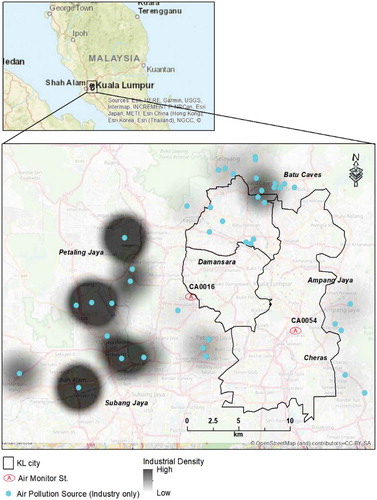
The major industrial pollutant sources are delineated by the nearest feasible radius surrounding the receptor. These sources include food and beverage sector, automobile maintenance and services, chemical industry, as well as a complex road network (Figure 1). ArcGIS software was used to map the study area and relative locations of the roads, main emission sources, and industrial areas to the monitoring site and measure the distances to the receptor station.

One-hour air quality data of SO₂, NO_x, CO, and PM10 were collected from 1 January 2016 to 31 December 2016 from the site, analyzed and used throughout this study. Table 1 shows data from stations CA0016 and CA0054. All pollutants were measured in volumetric units ppm, except PM10 which was measured in Gravimetric unit (µg/m³). Wind speed registered at Max. value of 26.5 m/sec at CA0054 and Min. value of 0.7 m/sec at CA0016.

3.1. Missing data imputation

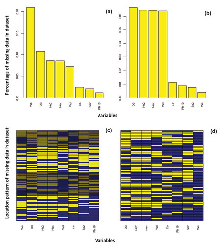
Data from 1 January 2016 to 31 December 2016 were collected from two air monitoring stations, CA0016 and CA0054, and used as input data for preliminary analysis (Figure 2). The data record contains hourly API values of PM10, SO₂, O₃, NO₂, and CO, in addition to other two meteorological parameters, ambient temperature (°C) and humidity (%), in KL city (northern Malaysia).

Figure 2. Missing data summary (a) CA0054 and (b) CA0016 and the pattern of the missing data (c) CA0054 and (d) CA0016 along the data record period of the mean values of the pollutants for the period 2007 to 2016. (Yellow color indicates missing data while blue color indicates existing data).

The R package, MICE, imputes incomplete multivariate data by chained equations (Buuren and Groothuis-Oudshoorn 2010; Shah et al. 2014), using predictive mean matching (PMM) for multiple imputation of missing data (Rubin and Schenker 1986). Its effective data manipulation capabilities make R very suitable for analyzing air pollution data to manage air pollution (Carslaw and Ropkins 2012).

The acquired data records were examined to detect missing data that need to be imputed before processing. Using 2 stations to encircle the study area, we collected records of days, containing the largest amount of missing data in 10 years. Wind speed had the maximum value of missing data, which reached 20% in station CA0054, as shown in Figure 2. The missing data for the rest of the variables (pollutants and wind speed) vary but do not exceed 10%. Generally, the missing data are moderate and the data imputation technique used in this study is applicable to cover this level of uncertainty. This is because the PMM generates imputed values that are very similar to real values. Imputations are based on values observed elsewhere, so they are realistic. This forecloses the possibility of imputations outside the observed data range, thus avoiding issues with invalid imputations (Buuren and Groothuis-Oudshoorn 2010; Allison 2015).

3.2. Decision tree (DT)

Random Forest’s (RF) multiple models have been successfully used to model air pollutants (Kumar 2018; Kamińska 2018; Chen et al. 2018) and were adopted in this research.

Classification and Regression Trees (CART) packages use many algorithms to plot a simplified pruned tree that split attributes based on sum of squared error values that minimize a loss function. rpart (Brieman et al. 1984) was used to plot classification trees. This is preferable because the other models have complex tree leaves, which are impractical to include. Breiman et al.’s method has been successfully implemented in past and present studies in diverse areas (Zhao et al. 2018; Cheng et al. 2018; Barlin et al. 2013). The following sequential procedures were implemented in this study:

• API was used in place of real values for the pollutants, while the real values of humidity and ambient temperature were utilized.

• In environmental research, missing data are the first source of uncertainty. It is therefore necessary for the data supplier to perform a data imputation process.

• The PMM in MICE package used to impute missing values was selected based on the numeric variable type of data.

• The acquired data were prepared and exported to the R environment. The DT algorithms, rpart and randomforest, as well as the air pollution algorithm, openair, were also utilized.

• Data scaling was performed on API of PM10 and other pollutants CO, SO₂, and NO_x. Hourly data were converted into 10 percentile values to focus on revealing the inter-correlation between API of leading pollutants and other pollutants’ API ranges (Figure 3).

  Figure 3. (a) PM10 percentile distribution at CA0016 and (b) PM10 percentile distribution at CA0054. X-axis represents percentile unit while y-axis represents the frequency of the units.

  

• To plot decision tree classification and run random forest algorithm, the entire data (without sampling) were initially used. However, due to the enormous size of the tree which made it unreadable on A4 or letter paper scale as well as the cumbersome relationship between the variables and the resultant multiple parent and child nodes, we optimized the size and processing time by subsetting 1000 randomly selected hours to produce the classification rules.

3.3. Bivariate cluster polar function

Bivariate polar plots indicate joint variations in concentration of species with wind speed and direction in polar coordinates, offering a valuable graphical technique for extracting directional information on pollutants’ sources (Carslaw and Beevers 2013). In addition to its common application for the assessment of dependence of pollutants’ concentrations on wind speed and direction, the enhanced polarPlot function is increasingly being used for newer applications such as source identification (Westmoreland et al. 2007; Carslaw et al. 2006), identification of features in a polar plot with similar characteristics (Carslaw and Beevers 2013), and extraction of additional information from the plots (Uria-Tellaetxe and Carslaw 2014). In this research, we complemented the polar plot function with the k-means polar clustering function. This is to overcome the limitations of the polarPlot function, which is mainly able to identify interesting features requiring further analyses. While the polarPlot is able to select areas of interest based only on a consideration of a plot that is determined by wind direction and wind speed intervals, the k-means clustering can identify, select, and group similar bivariate polar plot features together, as well as identify sources of pollution. We implemented the Elbow method (Charrad et al. 2014) to group data for better representation of likely pollution source traits. Care was taken to ensure that the distance between points in a cluster in comparison to the distance between the clusters was minimal. This is due to the influence of distance measure on the effectiveness of clustering.

3.3.1. Elbow method

Specifying the number of clusters k to be generated is essential in partitioning clustering. The direct method of establishing an optimal number of clusters via assessment of the generated dendrogram utilizing hierarchical clustering was adopted.

Specifically, the Elbow method, which defines clusters through the minimization of the total intra-cluster variation or total within-cluster sum of square (WSS) was utilized. The total WSS measures the compactness of the clustering, with a preference for small values. The Elbow clustering technique considers the total WSS as a function of the available number of clusters.

The optimal number of clusters was stipulated using the following procedures:

1. We computed the k-means clustering for different values of k. by varying its value from 1 to 10 clusters.

2. The WSS value for each k was computed.

3. The WSS curve was plotted based on the number of clusters k.

The appropriateness of the number of clusters was established through the appearance of a bend (knee) in the plot.

In summary, we applied K-means clustering method to understand the common directions of the selected pollutants together with wind speed and wind direction with each pollutant that was recommended based on the results obtained from the decision tree analysis (SO₂, CO, and PM10).

Thereafter, we determined the optimized number of clusters that yield the maximum number of varieties in the data distribution using the Elbow method. Figure 4 shows similar number of clusters using entire period for 3 pollutants’ data (PM10, SO₂, CO). Based on the recommended clustering number, 4 to 5 clusters are sufficient to summarize the clusters’ condition of the existing data, particularly if the CAQMs are located in rural areas with low quantity of pollutants. However, whenever there are sensitive cases of clusters, for instance, complexity of pollutants’ sources distribution, existence of a single source that may emit different pollutants such as industrial zones with factories comprising complex processing units of different products, or unclassified land uses (for example, mixture of commercial and industrial zones), the accuracy of measurements can be enhanced by increasing the clusters to reach the threshold. Since this study’s CAQM’s are surrounded by a complex structure of pollutants, increasing the number of clusters (preferably more than a threshold of 4) will give a clear indication of even small quantities of pollution. Therefore, a higher number of clusters (8–10) was adopted to highlight any sensitive changes between the data value of each pollutant.

Figure 4. Elbow algorithm to show the best number of clusters in CA0016 station using normalize percentiles quantiles of (a) SO₂; (b) PM10; (c) CO.

3.4. The TheilSen function

Calculating trends for air pollutants provides an overview of changes in pollutants’ concentration with time. The commonly used ordinary linear regression has several pitfalls such as the assumption of normality, autocorrelation, etc. However, modern regression methods make up for the limitations of older ones by incorporating the strengths of non-parametric methods and bootstrap simulations (Wilcox 2010). This research used the Theil-Sen method for trend computation. Given a set of n x, y pairs, the slopes between all pairs of points are calculated. Note that the number of slopes can increase by ≈n2. This implies that an increase in the length of the dataset will yield a rapid increase in the number of slopes. The Theil-Sen algorithm estimates the median of all the slopes under consideration. Theil-Sen estimator has two vital features for air pollution application: 1) generation of accurate confidence intervals even with non-normal data and heteroscedasticity (non-constant error variance); 2) resistance to outliers. In openair, we adopted (Kunsch 1989) approach of setting the block length to n1/3 where n is the length of the time series. We also used Bootstrap resampling to derive estimate of p for the slope. The trend functions used in the current research are represented as mean concentration versus time, typically, by year. This type of analysis is essential for understanding changes in pollutants’ concentrations over time and for cross-comparison of air quality limits, standards, and regulations.

3.5. Time variation plot

Pollutants’ temporal variation can provide nuggets of information on potential air pollution sources. For instance, road vehicle emissions are predisposed to follow very regular patterns. This contrasts with some industrial pollutants from natural sources such as sea salt aerosol, which are likely to exhibit significantly different patterns. Time variation plot can be used to consider the differences between two or more pollutants based on time series, which will have multiple benefits. Evaluating these differences has the potential to reveal the character of each pollutant.

The plots also display the 95% confidence interval in the mean. These uncertainty limits are useful in establishing differences between pollutants’ sources. Bootstrap re-sampling was used to determine the uncertainty intervals. This approach calculates better estimates than using assumptions based on normality, especially in instances of limited data availability. A few input variables were considered by the function. It was unnecessary to normalize the concentrations again since we already normalized the parameters to 10 percentiles. Based on this, we were able to characterize air pollution for the pollutants considered in this study using variations in time. We also characterized the temporal features of pollutant sources and contrasted it with another subset of conditions.

4. Results and discussion

The following missing data were detected at station CA0016: 8% in O₃, NO₂, NO_x, and WD, respectively, while the rest of pollutants have missing data less than 1%. At station CA0054, we detected much higher amount of missing data, mainly represented by wind speed (20%), while O₃, NO₂, NO_x, and wind direction had 10% missing data. The other pollutants had less than 5% missing information. The behavior of the imputed values produced by PPM is similar to the observed values, for instance, the maximum and minimum values bounded by the real values. Also whenever there is a skew in observed values, the imputed values follow the same behavior. Figure 5 shows the entire period for both stations after we performed the imputation process.

Figure 5. Summary plot shows the mean values of the pollutants for the period 2007 to 2016 (a) CA0016, (b) CA0054.

Where “0%” in the bracket behind the missing value refers to ratio of missing data ([number of missing days’ record]/[total record period]) using real number precision.

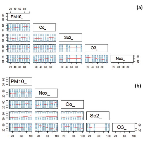
Pair plot is the first assessment to give an insight on the distribution of the pollutants and their behaviors. We created subset of the 1000 samples, normalized on percentile-based pollutants that were randomly selected on hourly basis to plot the trees. This represents the real data, without taking the mean that will negatively reduce the precision.

Figure 6(a) shows that in station CA0016, a direct and positive linear relationship exists between the PM10 (target pollutant) and CO, SO₂. Whereas, the SO₂ and CO show the same relationship, and this is the primary guide for common source and intensity trend. On the other hand, a semi-linear relationship is observed between the PM10 and others (O₃ and NO_x) while humidity shows a negative linearity with PM10. In a related study on air pollution in Lanzhou, China (Filonchyk, Yan, and Xiaojun 2018) reported an average correlation between PM10 and SO₂ while a negative relationship was observed between PM10 and O₃, which is not entirely different from this study’s outcome. They also observed a strong correlation between SO₂ and CO. With respect to meteorology, a weak positive or negative correlation between meteorological factors and air pollutants was observed in Lanzhou, reflecting a minimal impact of the factors on pollutants’ concentration although Guo et al. (2011) suggested stronger relationships with meteorological parameters in an earlier study. Further investigation is thus required to have more insights on the influence of humidity and other meteorological conditions on air pollutants in Kuala Lumpur. Findings from station CA0054 (Figure 6(b)) are almost similar, establishing the validity of using pair plot for insight purposes.

Figure 6. Pairplot relationship between CO, PM10, humidity, and SO₂ (a) CA0016 (b) CA0054.

Randomly selected hourly based subset show more realistic values in comparison to aggregate functions. This is because using the data that is generalized as daily aggregated values will cause permanent loss of significance of hour-based data. Also, real data will be lost while with subset, randomly selected real data can be retained.

4.1. Decision trees (DT)

Using DT (Rpart) algorithm to find the correlated pollutants with PM10, Figure 7(a) shows the tree of CA0016 could classify 10% of subset of 1000 using SO₂. The low PM10 percentile matches the low percentile of SO₂ and CO, while the highest quantiles matches the O₃ highest quantile. Figure 7(b) confirmed this observation by successfully classifying 13% of the data and proposed SO₂ and CO to confirm the dependent behavior with PM10 while O₃ gives a non-constant classification for PM10, which considers it as a less effective predictor.

Figure 7. Decision tree using Rpart algorithms using 1000 randomly selected hours (a) CA0016 (b) CA0054.

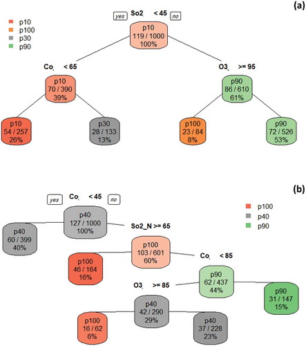
Random forest algorithm used the full data of 10 years to predict the most correlated pollutants to PM10 (Table 2), and we notice that SO₂ and CO considerably have the highest prediction performance compared to NOx and O3 for both stations. In their study, Rodríguez, Dupont-Courtade, and Oueslati (2016) showed that densely populated cities like Kuala Lumpur are characterized by higher concentration of SO₂.

Table 2. Pollutants’ relative importance according to PM10 using random forest results.

Station	CO	SO2	NOx	O3
CA0016	21	57	20	2
CA0054	51	40	0	9

4.2. Bivariate cluster polar function

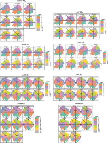
Figure 8 shows the clustering from lower to higher percentile mean values, where the highest cluster order refers to the highest pollution amount. Plots confirm that SO₂, CO, and PM10 within the same clusters have common directions in CA0016 station. Some concentrations become more obvious when we used 12 clusters. While in station CA0054 we see more independency for SO₂ and PM10 from other pollutants like NO_x and CO, which did not show any common relationship, presenting a misleading representation as well.

Figure 8. Polar cluster plot for CA0016 and CA0054 stations.

The outcome of the polar plot is presented in Figure 9. Here, the windspeed was substituted with attribute of cluster order. This plot will help us identify the direction of the clustered pollutants as well as the intensity value for each cluster, which is missing in Figure 8. Similar to this study, Bae et al. (2011) used the Conditional Polar function (CPF) technique to identify the direction of pollutants’ sources in relation to their concentrations at a rural site in New York while Henry et al. (2009) utilized a non-parametric wind regression approach for pollutants’ source identification and impact quantification. These methods work well in identifying known local point sources, with the CPF approach having an added advantage of easier computation (Kim and Hopke 2004). Comparing Figure 9 to Figure 8, it is interesting to note that the highest concentration value, as in Figure 9(a), can be detected by cluster 8 to the north-east. This aligns with the clustering of air pollution sources in the north-east in Figure 1. Assessing Figures 9 and 1, it can be deduced that the likely source of pollution is the city center location. While Fig. 8, with higher order of clustering, shows more clusters without identifying clearly the differences in concentration between these clusters; and whether it is valid to have more clustered order to classify new values in new groups. Results in Figure 9 confirmed that increase in the number of clusters will not always lead to significant results.

Figure 9. Polar plot with cluster instead of wind speed.

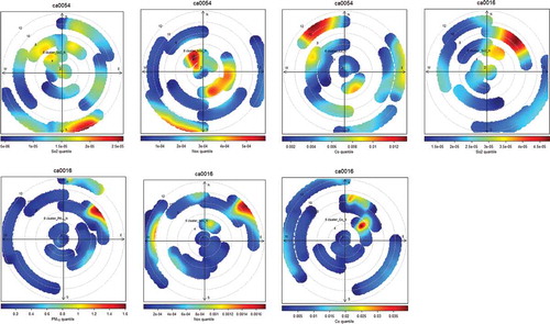
Our findings (Figure 9) also confirm the relationship between the direction and intensity of PM10 and SO₂ in station CA0016, while CO has shown a clear divergence. The strong correlation between PM10 and SO₂ is an indicator of the similarity in their origin, particularly traffic and industrial emissions as well as pollution induced by high energy consumption due to large population, all of which characterize many big cities (Filonchyk, Yan, and Xiaojun 2018; Rodríguez, Dupont-Courtade, and Oueslati 2016). Results at station CA0054 confirm the relationship observed in CA0016, as SE direction proved to emit the PM10 and SO₂ with the same relative intensity. With this observation, we confirm the need of polar cluster as an auxiliary and complete evidence to the previous findings. Further investigation is required to confirm the combined sources of PM10 and SO2. In CA0016, we noticed that the directions of PM10 and SO₂ for the last cluster are almost identical. For CA0054 station, we see CO is the highest correlated factor with lower contribution from SO₂ and null from NO_x, and this aligns with the findings from similar studies with DT. The high correlation with CO at this station is possibly due to the high traffic volume in the part of the city, being a major transportation hub connecting different states.

4.3. The TheilSen function

Figure 10 shows the deseasonalized monthly mean concentrations of pollutants at stations CA0016 and CA0054. Trend was measured by unit per year. The trend estimate is represented by the solid red lines while the dashed red lines indicate the 95% confidence intervals for the trend based on resampling methods. The overall trend is shown first before the slope value between brackets (ppb) per year and the 95% confidence intervals in the slope between brackets ppb/year. The three stars (∗ ∗ ∗) show that the trend is significant to the 0.001.

Figure 10. The Theil-Sen function plot for CA0016 and CA0054 stations. Y-axis represents the values of concentrations and X-axis represents the time in years.

Note also that the symbols shown next to each trend estimate relate to how statistically significant the trend estimate is: p < 0.001 = ∗ ∗ ∗, p < 0.01 = ∗∗, p < 0.05 = ∗, and p < 0.1 = +.

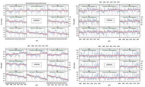
Figure 10. (Continued).

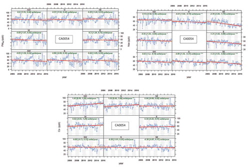
Results at station CA0016 that is surrounded by city center and other pollutants from all directions reveal a general increase in concentration trend in all directions, and the biggest trend (more than 1) was from N and NE (Figures 1 and 9). This is likely due to the high level of industry emission in these areas. SO₂ pattern proved the inter-correlation with PM10 has similar increment with 30% less, showing positive trend in NW, N, and NE, while southern directions exhibit an almost constant trend. Cluster plot (Figure 8) confirms the common direction and magnitude of the source of PM10 and SO₂. NO_x has more than 3 negative units’ trend to the south and around 2 positive units at the north. While CO, which received less weight (Table 2), has deviated in Figure 8 especially in S, SE, and SW. This confirms the finding of random forest algorithm that SO₂ received the highest importance weight with respect to PM10 (Table 2). While other pollutants (NOx) show different behavior in all directions, particularly the N, NE, and NW.

In station CA0054, PM10 generally shows a reduction in trend, especially in SW. The emitters situated at the north and North West also showed reduction in trend but in small amount. Overall, a minimal reduction in the pollutants’ concentration in all directions is observed (less than 1). This might be attributable to the distance to the pollutant sources since distance to areas of high industrial activities is a major influence of pollution (Tian, Yao, and Chen 2019). SO₂ has a similar trend with PM10 but with lower relative decline of intensity (less than 0.2). CO has the highest trend, observed in N and NW (more than 1), and slight intermittent reduction and increment in all directions. NO_x has a general trend reduction in all directions, while the highest trend increase occurred in the NE.

Similar changes in values of PM10 and SO₂ are indicated. When analyzed with cluster plot Figure 8, a confirmation of the common direction and magnitude of the sources of PM10 and SO₂ is obtained. This validates the findings of this research’s random forest algorithm that SO₂ received the highest importance weight in relation to PM10 (Table 1).

It is noteworthy that some pollutants did not record significant trend in some directions. This is because there is always a great excess of active pollutants, which might react to form other gases. For instance, NO reacts with O₃ to form NO₂.

We conclude that most of the serious pollutants show a positive trend toward the industrial areas in both stations, with negligible or constant trend elsewhere. A similar outcome was obtained by Liu et al. (2016) wherein the LUR model found a correlation between major pollutants and industrial areas. This is indicative of the nature of uncontrolled and unsustainable development in the densely populated areas of the city. Opening new areas for development out of the highly populated city center will likely reduce the emission of pollutants in the city center. According to Silva, Oliveira, and Leal (2016), the high rate of energy consumption in densely populated cities exacerbates air condition.

Stable or flat trend is an indication of pollutants being under control, either due to the fact that there were no new significant changes in the area or the effect was not impactful or traceable from the monitoring station.

4.4. Time variation plot

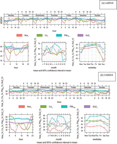
The normalized data from stations CA0016 and CA0054 (Figure 11) were used to detect the differences between two or more pollutants based on time series analysis. The top-left image depicts the diurnal variation of concentrations for all days. It reveals a constant behavior in PM10 and SO₂ concentrations along the data with slight increment between midnight and 6 AM. Fluctuations were observed in the behaviors of CO and NO_x during the day while SO₂ displayed relative stability. The shading shows the 95% confidence intervals of the mean. This suggests that the constant trend of PM10 and SO₂ is induced by dominant pollutant sources like industries as well as daily traffic emissions due to urban mobility. A similar scenario occurs in Lanzhou, where the high concentration of pollutants is attributed to traffic and industry emissions (Filonchyk, Yan, and Xiaojun 2018). On the other hand, weekly trends have common low values at the beginning of the week (Monday), rise constantly and drop down at the end of the week (Saturday and Sunday). The annual trend has significant effect on the PM10 and SO₂ distribution as evinced by the seasonal variation of its behavior, while CO and NO_x are less influenced by annual trend, displaying greater stability. In their study of air pollutants in Beijing based on hourly data derived from 35 monitoring stations, Tian, Yao, and Chen (2019) confirmed the influence of seasonal variations on the spatio-temporal dispersion of air pollutants.

For CO, there is a very pronounced increase in concentrations during the peak rush hour in the evenings and at night. It is interesting to note the trend on Sundays when CO concentrations are relatively much higher than NOx. This is attributable to the movement of mostly petrol-driven cars and diesel-driven vans and HGVs during the week, with a significant decline in the movement of these vehicles on Sundays. Although there is tendency for air pollutants to vary significantly across different months (Jiang et al. 2015; Filonchyk, Yan, and Xiaojun 2018), our study’s monthly trend is very similar in each case – which indicates very similar source origins and weather pattern. Taken together, the plots highlight the prevalence of traffic emissions at this site (CA0016) for CO and NOx, but there are important differences in how these emissions vary by hour of day and day of week.

Figure11(b) has shown a similar daily, weekly monthly and annual trend behavior, except that the concentration values relatively differ in scale compared to CA0016.

Figure 11. TimeVariation function for normalized concentrations of NO_x, CO, SO₂, and PM10 for (a) CA0016, (b) CA0054. Y-axis represents the normalized values of concentrations and X-axis represents the time in hour, months, and days.

4.5. Implications of findings for sustainable air pollution reduction and management

Atmospheric pollutants exhibit a complex and complicated relationship especially when they have multiple nonpoint sources, and come in contact with meteorological parameters. Likewise, the urban atmosphere of Kuala Lumpur city and parts of Selangor state has for long portrayed huge concentration in the size and composition of pollutants. These complexities and data matrix composition make it very difficult to produce a well-precise representation. In view of this, the findings of this study introduce several machine learning algorithms that are more precise than ordinary statistical technique. This is because hidden latent behaviors of pollutants relationships with meteorological conditions are difficult to understand. In KL, for instance, a general increase in the trend of pollutant was noticed in the north and north-eastern direction indicating a dispersion capability of wind. This means that wind can transport pollutants from point source to nonpoint source. For a sustainable air pollution reduction and management, it is imperative to put into consideration the fact that apart from pollutant emission from a given source, wind as a meteorological factor can change the dimension and direction of the pollutants. As such, the attention of stakeholders is drawn to enforce policies on clean air adoption in order to reduce the size, number, and concentration of the pollutants. This measure will minimize the pollutants dispersed by wind movement.

It was also observed that the sensitive pollutants used for this study retain a continuous increase in size, number, and composition within the industrial layouts located in the stations compared with the vicinity of the study area. This is because industries play a significant role in releasing pollutants during manufacturing processes. Thus, this study proposes a new shift in policy making and implementation by government to adopt a new industrial layout in order to decongest the already overcrowded, uncontrolled, and unstained clustering of industry. Likewise, it is important for industries to adopt means of reducing gas emission and green technology that can help in carbon sink as well as prevent high pollution. This will help to simplify and minimize the rate of pollutant emission for a sustained air pollution control.

Also, using the random forecast algorithm, it was observed that SO₂ and CO are the most discriminating parameters enhancing the concentration of PM10 as a secondary pollutant. This is an indication that vehicular emissions due to traffic congestion especially during the workdays produce high concentration of PM10 precursors that accelerate the high concentration of pollution. This is due to constant increase in the number of private ownership of vehicles that are responsible for the emission of these pollutants. For instance, it is discovered that there is a sharp drop in pollutant concentration during the weekend because most household vehicles are parked at home. In addition, there is an increase in CO concentration during the peak rush hour of evening and night because most people return from work during that period, since CO is mostly produced by incomplete combustion of fuel containing carbon. Investment should be made in utilizing non-fuel-powered vehicles such as solar and electrical engines. For sustainable air quality, catalyst converter can be introduced as a new dimension toward maintaining clean air. The government can also introduce additional public transport system that will reduce excess pollutant emission from individual car owners. This will in turn reduce the number of private vehicle ownership thereby regulating the rate at which anthropogenic induced pollutants are emitted. Consequently, the cost of maintaining roads, accidents, traffic congestion, and other related health risk implications could be minimized. Adopting such measures will change the pattern and composition of pollutants for sustainable air quality management and control.

Providing clean air, good quality environment, and life-long health assurance is essential for sustainable living and key players including government and non-governmental organizations should be willing to adopt measures capable of reducing air pollutant emission and mitigating its impacts. Understanding the dynamics and complexities in ambient air relationships is crucial to achieving this. This study’s findings provide evidence-based insights on the inter-correlations and significance of major pollutants in Kuala Lumpur, with the potential to support a sustainable air pollution reduction and management strategy in the city, which can be adopted in other major cities around the world.

5. Conclusion

In the current study, we introduced multiple machine learning algorithms to test the inter-correlation between dominant API for PM10 percentile values and other air pollutants SO₂, O₃, NO_x, and CO, in Malaysia’s capital city, Kuala Lumpur, and surrounding areas using data from 2007 to 2016. The study found that SO₂ is the major pollutant significantly inter-correlating with PM10, while CO and NO_x have major different sources that contribute to degradation of air quality in the study area mainly due to the combustion process from transportation modes like private vehicles and developing industries. RPART and Random forest algorithms performed well by producing clear information about the most important variables that inter-correlate with PM10 API value.

This research’s use of machine learning decision trees for environ-metric analysis facilitated better understanding of main pollutants contributing to the high API value in the study area. Specifically, the following findings were observed:

• Some pollutants have relatively small values, thus using 10 percentiles enables us to compare the changes as the scaling function as well as detect the small changes in frequency without reducing the clarity using the polar plots alone will not give high confidence to decision-makers, as the pollutants may have a common relationship with 1st, 2nd, and 3rd quantiles but not all with the 1st.

• Pair plots serve as a useful guide to study the behavior of pollutants in-relation with each other.

• Common pollutants show similar cluster number and directions.

• All the presented results proved the correlation between PM10 and SO₂ in magnitude and direction.

• Most of the sensitive pollutants have a positive trend toward the industrial areas in both stations, with no or constant trend elsewhere. This pattern is indicative of the nature of development in the city, which is more focused on further developing already dense areas rather than develop new areas out of the highly populated city center.

• Trend of PM10 and SO₂ can be detected by annual changes, while weekly and daily trend may reflect better discrimination for CO and NO_x.

R programing environment shows impressive reliability in terms of availability of various decision trees algorithms and processing air pollution data. In future, more data and further analysis are required to better understand why NO₂ shows mildly important results. Also, the incorporation of wind direction and speed has the potential to contribute added value to our current findings.

Acknowledgements

The authors gratefully acknowledge the financial support from the University Teknologi PETRONAS (UTP) STIRF research grant [0153AA-F83] for this project. Also, we are very grateful to Department of Environment (DoE), Malaysia, for providing the air quality data used in this study and the Federal Department of Town and Country Planning (PLANMalaysia) for providing spatial and attribute data of the study area.

Disclosure statement

No potential conflict of interest was reported by the authors.

Additional information

Funding

This work was supported by the Universiti Teknologi PETRONAS (UTP) STIRF research grant [0153AA-F83].

References

- Afzali, A., M. Rashid, M. Afzali, and V. Younesi. 2017. “Prediction of Air Pollutants Concentrations from Multiple Sources Using AERMOD Coupled with WRF Prognostic Model.” Journal of Cleaner Production 166: 1216–1225. doi:10.1016/j.jclepro.2017.07.196.
- Allison, P. 2015. “Imputation by Predictive Mean Matching: Promise & Peril.” Statistical Horizons, Accessed 12 September 2019. https://statisticalhorizons.com/predictive-mean-matching
- Althuwaynee, O. F., and B. Pradhan. 2017. “Semi-quantitative Landslide Risk Assessment Using GIS-based Exposure Analysis in Kuala Lumpur City.” Geomatics, Natural Hazards and Risk 8 (2): 706–732.
- Althuwaynee, O. F., W. Musakwa, T. Gumbo, and S. Reis. 2017. “Applicability of R Statistics in Analyzing Landslides Spatial Patterns in Northern Turkey.” 2nd International Conference on Knowledge Engineering and Applications (ICKEA). Imperial College London, London, United Kingdom.
- Awang, M. B., A. B. Jaafar, A. M. Abdullah, M. B. Ismail, M. N. Hassan, R. Abdullah, S. Johan, and H. Noor. 2000. “Air Quality in Malaysia: Impacts, Management Issues and Future Challenges.” Respirology 5 (2): 183–196. doi:10.1046/j.1440-1843.2000.00248.x.
- Bae, M.-S., J. J. Schwab, W.-N. Chen, C.-Y. Lin, O. V. Rattigan, and K. L. Demerjian. 2011. “Identifying Pollutant Source Directions Using Multiple Analysis Methods at a Rural Location in New York.” Atmospheric Environment 45 (15): 2531–2540. doi:10.1016/j.atmosenv.2011.02.020.
- Barlin, J. N., Q. Zhou, C. M. S. Clair, A. Iasonos, R. A. Soslow, K. M. Alektiar, M. L. Hensley, M. M. Leitao Jr, R. R. Barakat, and N. R. Abu-Rustum. 2013. “Classification and Regression Tree (CART) Analysis of Endometrial Carcinoma: Seeing the Forest for the Trees.” Gynecologic Oncology 130 (3): 452–456. doi:10.1016/j.ygyno.2013.06.009.
- Brieman, L., J. Friedman, R. Olshen, and C. Stone. 1984. “Classification and Regression Trees. Belmont (CA): Wadsworth. Google Scholar.
- Brodny, J., and M. Tutak. 2019. “Analysis of the Diversity in Emissions of Selected Gaseous and Particulate Pollutants in the European Union Countries.” Journal of Environmental Management 231: 582–595. doi:10.1016/j.jenvman.2018.10.045.
- Buuren, S. V., and K. Groothuis-Oudshoorn. 2010. “Mice: Multivariate Imputation by Chained Equations in R.” Journal of Statistical Software, 45 (3): 1–68.
- Carslaw, D. C., and K. Ropkins. 2012. “Openair—An R Package for Air Quality Data Analysis.” Environmental Modelling & Software 27: 52–61. doi:10.1016/j.envsoft.2011.09.008.
- Carslaw, D. C., and S. D. Beevers. 2013. “Characterising and Understanding Emission Sources Using Bivariate Polar Plots and K-means Clustering.” Environmental Modelling & Software 40: 325–329. doi:10.1016/j.envsoft.2012.09.005.
- Carslaw, D. C., S. D. Beevers, K. Ropkins, and M. C. Bell. 2006. “Detecting and Quantifying Aircraft and Other On-airport Contributions to Ambient Nitrogen Oxides in the Vicinity of a Large International Airport.” Atmospheric Environment 40 (28): 5424–5434. doi:10.1016/j.atmosenv.2006.04.062.
- Chaloulakou, A., I. Mavroidis, and I. Gavriil. 2008. “Compliance with the Annual NO2 Air Quality Standard in Athens. Required NOx Levels and Expected Health Implications.” Atmospheric Environment 42 (3): 454–465. doi:10.1016/j.atmosenv.2007.09.067.
- Charrad, M., N. Ghazzali, V. Boiteau, A. Niknafs, and M. M. Charrad. 2014. “Package ‘nbclust’.” Journal of Statistical Software 61: 1–36.
- Chen, G., Y. Wang, S. Li, W. Cao, H. Ren, L. D. Knibbs, M. J. Abramson, and Y. Guo. 2018. “Spatiotemporal Patterns of PM10 Concentrations over China during 2005–2016: A Satellite-based Estimation Using the Random Forests Approach.” Environmental Pollution 242: 605–613. doi:10.1016/j.envpol.2018.07.012.
- Cheng, Z., M. Nakatsugawa, H. Chen, S. P. Robertson, X. Hui, J. A. Moore, M. R. Bowers, A. P. Kiess, B. R. Page, and L. Burns. 2018. “Evaluation of Classification and Regression Tree (CART) Model in Weight Loss Prediction following Head and Neck Cancer Radiation Therapy.” Advances in Radiation Oncology 3 (3): 346–355. doi:10.1016/j.adro.2017.11.006.
- de Rooij, M. M. T., D. J. J. Heederik, F. Borlée, G. Hoek, and I. M. Wouters. 2017. “Spatial and Temporal Variation in Endotoxin and PM10 Concentrations in Ambient Air in a Livestock Dense Area.” Environmental Research 153: 161–170. doi:10.1016/j.envres.2016.12.004.
- Dominick, D., H. Juahir, M. T. Latif, S. M. Zain, and A. Z. Aris. 2012. “Spatial Assessment of Air Quality Patterns in Malaysia Using Multivariate Analysis.” Atmospheric Environment 60: 172–181. doi:10.1016/j.atmosenv.2012.06.021.
- Filonchyk, M., H. Yan, and L. Xiaojun. 2018. “Temporal and Spatial Variation of Particulate Matter and Its Correlation with Other Criteria of Air Pollutants in Lanzhou, China, in Spring-summer Periods.” Atmospheric Pollution Research. doi:10.1016/j.apr.2018.04.011.
- Fortelli, A., N. Scafetta, and A. Mazzarella. 2016. “Influence of Synoptic and Local Atmospheric Patterns on PM10 Air Pollution Levels: A Model Application to Naples (Italy).” Atmospheric Environment 143: 218–228. doi:10.1016/j.atmosenv.2016.08.050.
- Guo, Y., F. She, S. Wang, B. Liu, J. Li, and J. Wang. 2011. “Assessment on Air Quality in Lanzhou and Its Relation with Meteorological Conditions.” Journal of Arid Land Resources and Environment 25 (11): 100–105.
- Henry, R., G. A. Norris, R. Vedantham, and J. R. Turner. 2009. “Source Region Identification Using Kernel Smoothing.” Environmental Science & Technology 43 (11): 4090–4097. doi:10.1021/es8011723.
- Ibrahim, M. Zamri., M. Ismail, and Y. K. Hwang. (2012). Mapping The Spatial Distribution Of Criteria Air Pollutants in Peninsular Malaysia Using Geographical Information System (GIS). Intech. Available at: https://www.intechopen.com/books/air-pollution-monitoring-modelling-and-health/mapping-the-spatial-distribution-of-criteria-air-pollutants-in-peninsular-malaysia-using-geographica
- Jiang, D., Y. Zhang, H. Xiang, Y. Zeng, J. Tan, and D. Shao. 2004. “Progress in Developing an ANN Model for Air Pollution Index Forecast.” Atmospheric Environment 38 (40): 7055–7064. doi:10.1016/j.atmosenv.2003.10.066.
- Jiang, W., Y. Wang, M.-H. Tsou, and F. Xiaokang. 2015. “Using Social Media to Detect Outdoor Air Pollution and Monitor Air Quality Index (AQI): A Geo-targeted Spatiotemporal Analysis Framework with Sina Weibo (Chinese Twitter).” PloS One 10 (10): e0141185. doi:10.1371/journal.pone.0141185.
- Kamińska, J. A. 2018. “The Use of Random Forests in Modelling Short-term Air Pollution Effects Based on Traffic and Meteorological Conditions: A Case Study in Wrocław.” Journal of Environmental Management 217: 164–174. doi:10.1016/j.jenvman.2018.03.094.
- Kim, E., and P. K. Hopke. 2004. “Comparison between Conditional Probability Function and Nonparametric Regression for Fine Particle Source Directions.” Atmospheric Environment 38 (28): 4667–4673. doi:10.1016/j.atmosenv.2004.05.035.
- Kumar, D. 2018. “Evolving Differential Evolution Method with Random Forest for Prediction of Air Pollution.” Procedia Computer Science 132: 824–833. doi:10.1016/j.procs.2018.05.094.
- Kunsch, H. R. 1989. “The Jackknife and the Bootstrap for General Stationary Observations.” The Annals of Statistics 1217–1241. doi:10.1214/aos/1176347265.
- Latif, M. T., D. Dominick, F. Ahamad, M. F. Khan, L. Juneng, F. M. Hamzah, and M. S. M. Nadzir. 2014. “Long Term Assessment of Air Quality from a Background Station on the Malaysian Peninsula.” Science of the Total Environment 482: 336–348. doi:10.1016/j.scitotenv.2014.02.132.
- Lee, S., and B. Pradhan. 2007. “Landslide Hazard Mapping at Selangor, Malaysia Using Frequency Ratio and Logistic Regression Models.” Landslides 4 (1): 33–41. doi:10.1007/s10346-006-0047-y.
- Liu, C., B. H. Henderson, D. Wang, X. Yang, and Z.-R. Peng. 2016. “A Land Use Regression Application into Assessing Spatial Variation of Intra-urban Fine Particulate Matter (PM2. 5) and Nitrogen Dioxide (NO2) Concentrations in City of Shanghai, China.” Science of the Total Environment 565: 607–615. doi:10.1016/j.scitotenv.2016.03.189.
- Manimaran, P., and A. C. Narayana. 2018. “Multifractal Detrended Cross-correlation Analysis on Air Pollutants of University of Hyderabad Campus, India.” Physica A: Statistical Mechanics and Its Applications 502: 228–235. doi:10.1016/j.physa.2018.02.160.
- Meraz, M., E. Rodriguez, R. Femat, J. C. Echeverria, and J. Alvarez-Ramirez. 2015. “Statistical Persistence of Air Pollutants (O3, SO2, NO2 and PM10) in Mexico City.” Physica A: Statistical Mechanics and Its Applications 427: 202–217. doi:10.1016/j.physa.2015.02.009.
- Mohamad, N. D., Z. H. Ash’aari, and M. Othman. 2015. “Preliminary Assessment of Air Pollutant Sources Identification at Selected Monitoring Stations in Klang Valley, Malaysia.” Procedia Environmental Sciences 30: 121–126. doi:10.1016/j.proenv.2015.10.021.
- Murena, F. 2004. “Measuring Air Quality over Large Urban Areas: Development and Application of an Air Pollution Index at the Urban Area of Naples.” Atmospheric Environment 38 (36): 6195–6202. doi:10.1016/j.atmosenv.2004.07.023.
- Nazif, A., N. I. Mohammed, A. Malakahmad, and M. S. Abualqumboz. 2018. “Regression and Multivariate Models for Predicting Particulate Matter Concentration Level.” Environmental Science and Pollution Research 25 (1): 283–289. doi:10.1007/s11356-017-0407-2.
- Rodríguez, M. C., L. Dupont-Courtade, and W. Oueslati. 2016. “Air Pollution and Urban Structure Linkages: Evidence from European Cities.” Renewable and Sustainable Energy Reviews 53: 1–9. doi:10.1016/j.rser.2015.07.190.
- Rubin, D. B., and N. Schenker. 1986. “Multiple Imputation for Interval Estimation from Simple Random Samples with Ignorable Nonresponse.” Journal of the American Statistical Association 81 (394): 366–374. doi:10.1080/01621459.1986.10478280.
- Sanusi, M. S. M., A. T. Ramli, W. M. S. W. Hassan, M. H. Lee, A. Izham, M. N. Said, H. Wagiran, and A. Heryanshah. 2017. “Assessment of Impact of Urbanisation on Background Radiation Exposure and Human Health Risk Estimation in Kuala Lumpur, Malaysia.” Environment International 104: 91–101. doi:10.1016/j.envint.2017.01.009.
- Shah, A. D., J. W. Bartlett, J. Carpenter, O. Nicholas, and H. Hemingway. 2014. “Comparison of Random Forest and Parametric Imputation Models for Imputing Missing Data Using MICE: A CALIBER Study.” American Journal of Epidemiology 179 (6): 764–774. doi:10.1093/aje/kwt312.
- Shakir, S. K., A. Azizullah, W. Murad, M. K. Daud, F. Nabeela, H. Rahman, S. Ur Rehman, and D.-P. Häder. 2016. “Toxic Metal Pollution in Pakistan and Its Possible Risks to Public Health.” In de Voogt P. (eds) Reviews of Environmental Contamination and Toxicology Volume 242. Reviews of Environmental Contamination and Toxicology (Continuation of Residue Reviews), vol 242. Springer, Cham
- Silva, M., V. Oliveira, and V. Leal. 2016. “Urban Morphology and Energy: Progress and Prospects.” Urban Morphology 20:72–73.
- Sulong, N. A., M. T. Latif, M. F. Khan, N. Amil, M. J. Ashfold, M. I. A. Wahab, K. M. Chan, and M. Sahani. 2017. “Source Apportionment and Health Risk Assessment among Specific Age Groups during Haze and Non-haze Episodes in Kuala Lumpur, Malaysia.” Science of the Total Environment 601: 556–570. doi:10.1016/j.scitotenv.2017.05.153.
- Sun, X. W., P. L. Chen, L. Ren, Y. N. Lin, J. P. Zhou, N. Lei, and Q. Y. Li. 2018. “The Cumulative Effect of Air Pollutants on the Acute Exacerbation of COPD in Shanghai, China.” Science of the Total Environment 622: 875–881. doi:10.1016/j.scitotenv.2017.12.042.
- Tian, Y., X. Yao, and L. Chen. 2019. “Analysis of Spatial and Seasonal Distributions of Air Pollutants by Incorporating Urban Morphological Characteristics.” Computers, Environment and Urban Systems 75: 35–48. doi:10.1016/j.compenvurbsys.2019.01.003.
- Uria-Tellaetxe, I., and D. C. Carslaw. 2014. “Conditional Bivariate Probability Function for Source Identification.” Environmental Modelling & Software 59: 1–9. doi:10.1016/j.envsoft.2014.05.002.
- Westmoreland, E. J., N. Carslaw, D. C. Carslaw, A. Gillah, and E. Bates. 2007. “Analysis of Air Quality within a Street Canyon Using Statistical and Dispersion Modelling Techniques.” Atmospheric Environment 41 (39): 9195–9205. doi:10.1016/j.atmosenv.2007.07.057.
- Wilcox, R. R. 2010. Fundamentals of Modern Statistical Methods: Substantially Improving Power and Accuracy. New York: Springer.
- Yubero, E., A. Carratalá, J. Crespo, J. Nicolás, M. Santacatalina, S. Nava, F. Lucarelli, and M. Chiari. 2011. “PM10 Source Apportionment in the Surroundings of the San Vicente Del Raspeig Cement Plant Complex in Southeastern Spain.” Environmental Science and Pollution Research 18 (1): 64–74. doi:10.1007/s11356-010-0352-9.
- Zhang, J., L.-Y. Zhang, M. Du, W. Zhang, X. Huang, Y.-Q. Zhang, Y.-Y. Yang, J.-M. Zhang, S.-H. Deng, and F. Shen. 2016. “Indentifying the Major Air Pollutants Base on Factor and Cluster Analysis, a Case Study in 74 Chinese Cities.” Atmospheric Environment 144: 37–46. doi:10.1016/j.atmosenv.2016.08.066.
- Zhao, X., S. Barber, C. C. Taylor, and Z. Milan. 2018. “Classification Tree Methods for Panel Data Using Wavelet-transformed Time Series.” Computational Statistics & Data Analysis. doi:10.1016/j.csda.2018.05.019.