Influence of forest fire episodes on the distribution of gaseous air pollutants over Uttarakhand, India

ABSTRACT

Widespread forest fire events occurred in the foothills of North Western Himalaya during 24 April to 2 May 2016 (Event-1) and 20–30 May 2018 (Event-2). Their impacts were investigated on the distribution of pollutant gases ozone (O₃), carbon monoxide (CO), and oxides of nitrogen (NOx) over Uttarakhand using simulations of Weather Research and Forecasting model coupled with chemistry (WRF-Chem) and in-situ observations of these gases over Dehradun, the capital of Uttarakhand. During Event-1, the observed CO mixing ratio over Dehradun increased from 25 April 2016 onwards, attained maximum (705.8 ± 258 ppbv) on 2 May 2016 and subsequently decreased. The rate of increase of daily baseline CO was 29 ppbv/day during HFAP (High Fire Activity Period). During Event-2, daily average concentrations of CO, O₃, and NOx showed systematic increase over Dehradun during HFAP period. The rate of increase of CO was 9 ppbv/day, while it was very small for NOx and O₃. To quantitatively estimate the influence of forest fire emissions, two WRF-Chem simulations were made: one with biomass burning (BB) emissions and other without BB emissions. These simulations showed 52% (34%) enhancement in CO, 52% (32%) enhancement in NOx, and 11% (9%) enhancement in O₃ during HFAP for Event-1 (Event-2). A clear positive correlation (r = 0.89 for Event-1, r = 0.69 for Event-2) was found between ∆O₃ (O_{3with BB} minus O_{3without BB}) and ∆CO (CO_{with BB} minus CO_{without BB}), indicating rapid production of ozone in the fire plumes. For both the events, the vertical distribution of ∆O₃, ∆CO, and ∆NOx showed that forest fire emissions influenced the air quality upto 6.5 km altitude. Peaks in ∆O₃, ∆CO, and ∆NOx during different days suggested the role of varying dispersion and horizontal mixing of fire plumes.

KEYWORDS:

• Forest fires
• gaseous pollutants
• in-situ observation
• WRF-Chem and Dehradun

1. Introduction

Sporadic biomass burning (BB) episodes are the source of many air pollutants in the atmosphere. The significant amount of carbon monoxide (CO), oxides of nitrogen (NOx = NO+NO₂), methane (CH₄), and non-methane hydrocarbons (NMHCs) are released during such events. Their emissions significantly perturb the chemical weather on local, regional, and global scales (Crutzen and Andreae 1990; Andreae and Merlet 2001; Duncan 2003). They chemically produce secondary pollutant ozone, which is an oxidizing agent and greenhouse gas having potential climatic implications (Duncan 2003; Stone et al. 2008). Several research articles reported emissions of these trace gases and formation of secondary pollutants due to BB over Africa, America, Australia, and South-East Asia (Mauzerall et al. 1998; Takegawa et al. 2003; Kondo et al. 2004; Pfister, Wiedinmyer, and Emmons 2008). All these studies used different ground-based measurements, space-based observations, and chemical transport models to understand the impact of fire emissions on the surface air quality, atmospheric chemistry, and radiation budget. However, such efforts are limited over south Asia where BB significantly contributes in degradation of air quality, atmospheric chemistry, and radiation budget (Sahu and Sheel 2014; Pandey and Sahu 2014; Sahu et al. 2015).

The spatial and temporal distribution of BB varies in the tropical region according to forest cover and crop residue burning (van der Werf et al. 2010). In India, Northern, North-eastern, and central regions are hot spot areas of BB. Annually, forest fire burns 32–61 Tg/year and agricultural fire burns 116–289 Tg/year over India (Venkataraman et al. 2006). About 3.73 million ha of forest cover is prone to fire in the Indian region every year due to anthropogenic activities like shifting cultivation, burning agriculture and slash, fire wood burning, etc. (Bahuguna and Upadhay 2002; Chand et al. 2007). Widespread forest fires are great source of pollutant gases and aerosols in short span of time (Karathanassi, Andronis, and Rokos 2003; Hashim et al. 2004; Sharma, Kharol, and Badarinath 2011; Lu, Zhang, and Streets 2011; Calle, Salvador, and González-Alonso 2013; Reddington et al. 2014; Tomshin and Solovyev 2014; Shaik et al. 2019). Efforts have been made by Indian researchers to understand the impact of BB on the regional air quality using in-situ observations, satellite measurements, and chemistry transport modeling (CTM) (Beig et al. 2007; Ghude et al. 2008; Sharma et al. 2010; Ojha et al. 2014; Jena et al. 2015; Yarragunta, Srivastava, and Mitra 2017; Yarragunta et al. 2019). Due to obvious difficulty in in-situ measurements of air pollutants very close to forest fire affected areas, remote sensing observations provide very important information on their distribution (Ghude et al. 2008; Sharma et al. 2010; Ojha et al. 2014; Jena et al. 2015; Yarragunta, Srivastava, and Mitra 2017). They not only provide the spatial and temporal distribution of air pollutants over such locations (Tomshin and Solovyev 2014; Marlier et al. 2015; Thakur et al. 2019), but also provide active fire locations and land use/land cover (LULC) maps to identify the type and area of biomass burned (Abushenko et al. 2000; Sunar and Özkan 2001; Hansen et al. 2002; Friedl et al. 2002; Bartholomé and Belward 2005; Arino et al. 2008; Gleason and Im 2011; Wiedinmyer et al. 2011). These observations are required for the development of good BB emission inventories, which is an essential part of model simulations (Andreae and Merlet 2001; Giglio et al. 2010; Wiedinmyer et al. 2011; Ichoku, Kahn, and Chin 2012). Thus remotely sensed observations are very important part of CTM simulations (Al-Saadi et al. 2008; Roy and Boschetti 2009). CTMs play an important role in understanding the emission, transport, and transformation of fire plumes (Wu, Su, and Jiang 2011; Lei, Li, and Molina 2013; Cuchiara et al. 2017; Zhou et al. 2018). The sensitivity simulations of CTMs can be used to quantify the contribution of forest fire plumes on the air quality over the downwind regions (Park et al. 2009; Srivastava and Sheel 2013). Several efforts have been made by Indian researchers to understand the role of BB emissions on the degradation of air quality of adjoining regions (Ojha et al. 2014; Jena et al. 2015).

In the Himalayan region, coniferous forests were most vulnerable for forest fires where Chir Pine or blue Pine was highly abundant plant community and found at altitudes of 1000–1800 m (Vadrevu et al. 2012). The litters and pastures of Pine forests were generally burnt by local people during March–May to enhance the production of forage during monsoon. These fires severely affect the economy, public health, drying up water resources, and ecology of the region (Bahuguna and Upadhay 2002; Vadrevu et al. 2012). The widespread forest fires near foothills of Himalaya have significant impact on the hydrological cycle associated with monsoon rainfall over India (Nigam and Bollasina 2010; Vaux et al. 2012; Nair et al. 2013). Despite these important consequences, the current understanding on the effects caused by forest fires on air quality in the Himalayan region is limited. Kumar et al. (2011) investigated the influence of northern Indian BB on the air quality of Central Himalayas. However, their study included biomass over a larger Indian region which covered entire North India. In the present research work, we have investigated pollutants emitted from short duration intense forest fire episodes occurred over a region very close to North Western Himalayan glaciers. Two such events (Event-1: 24 April to 2 May 2016 and Event-2: 20 May to 30 May 2018) recently occurred and caused ecological loss as well as environmental and health issues over Uttarakhand. These intense forest fires occurred due to less than average rains in winter, followed by increase in temperature during April–May (Thakur et al. 2019). This resulted in accumulation of huge amount of dry litter and vegetation fuel. These meteorological conditions caused the spread of wildfire across the dense pine forest of Uttarakhand and created 3774.1 km² burnt area for Event-1 and 690.8 km² burnt area for Event-2. These events added many pollutants in the pristine environment of Uttarakhand. The role of these forest fires on local air quality have been investigated using in-situ observations and regional CTM simulations as well as quantify their contribution toward the pollution enhancement over Uttarakhand.

2. Methodology

2.1. Study region

Uttarakhand is a mountainous state in the northern part of India. Figure 1 shows its geographical location in India and has all the gradients of forest zones owing to different altitudes (180–7400 m). Uttarakhand has total forest cover of 24,240 km². This shares 43.3% state’s geographical area which is very high as compared to country’s share of 21.3% (Thakur et al. 2019). Chir pine forest, conifer forest, and oak forest are major forest types over this state (Singh et al. 2016). Forest fire activity over this region mostly occurs from February to June, with a peak in May–June period (Jha et al. 2016).

In the present study, measurements of trace gases are made at Indian Institute of Remote Sensing (IIRS), Dehradun (30° 32′N and 78° 03′E). Dehradun, the capital of Uttarakhand, is located in the south-western part of Uttarakhand state of India (Figure 1). It is situated in the center of Doon valley and bounded between Himalayas in the north and Shiwalik Hills in the south. The climate of Dehradun is humid sub-tropical where winters are very cold while summers are moderately hot. During summer, the average temperature is around 35–36°C and can rise upto 41°C . The detailed meteorology of this region can be found in Deep et al. (2019). The population of Dehradun is 1.7 million as per census 2011 and its growth rate per decade is estimated as more than 30% (https://www.census2011.co.in/census/district/578-dehradun.html). Dehradun environmental condition has worsen gradually due to increase in human activities such as deforestation, unplanned development, rapid population growth, increasing number of vehicles, urbanization, large-scale construction, etc. All these pollution sources contribute to degradation of air quality over Doon valley.

2.2. Measurements and model simulations

2.2.1. Surface measurements

Continuous in-situ measurements of trace gases were made using in-situ analyzers (Model: 42i for NOx, 48i for CO and 49i for O₃ Thermo Scientific, USA) since January 2018. The O₃ ultraviolet photometric analyzer works on the principle of absorption at 254 nm to measure the atmospheric O₃. The minimum detection limit of this analyzer is 1 ppbv with 20 s response time. The accuracy and precision of the measurements are 1 ppbv and ±5%, respectively. The CO analyzer works on the absorption property of CO at 4.67 µm. The minimum detectable limit of this instrument is 0.04 ppmv with 60 s response time. NO and NO₂ analyzer is based on chemi-luminescence technique. The response time of this instrument is 60 s with lower detectable limit of 50 pptv. Zero calibration and span calibration checks for these analyzers were performed on the regular basis using Zero air generator (Thermo Scientific’s Model 1160) and Multi-gas calibrator (Model: 146i).

HORIBA CO analyzer was used for the CO measurements in 2016. This analyzer works on the principle of cross modulation non-dispersive infrared absorption method. The minimum detection limit of this instrument is ~50 ppbv . The calibration of analyzer was carried out regularly to obtain accurate measurements.

2.2.2. WRF-Chem simulations

Weather Research Forecasting coupled with chemistry (WRF-Chem) version 3.9.1 is a state of the art numerical weather prediction system (Grell et al. 2004; Skamarock et al. 2008). This model was driven by several emission inventories and meteorological fields. In the present work, the NCEP final analysis fields (FNL) at a resolution of 1° × 1° had been used to provide meteorological initial and lateral boundary conditions to the model. MOZART-4 (Model for Ozone and Related Tracers Version-4) chemical mechanism was used to represent gas-phase chemistry in the model simulations (Emmons et al. 2010). Anthropogenic emissions were obtained from the Monitoring Atmospheric Composition and Climate (MACC)/CITYZEN (MACCity) emission inventory, available at a spatial resolution of 0.5° × 0.5° (Lamarque et al. 2010; Granier et al. 2011). The daily varying BB emissions of different trace species were taken from the Fire Inventory from NCAR (National Center for Atmospheric Research) (FINN) (Wiedinmyer et al. 2011). Biogenic emissions of trace species were calculated online using the Model of Emissions of Gases and Aerosols from Nature (MEGAN) (Guenther et al. 2006). The initial and boundary conditions of chemical species were taken from the MOZART-4 (Emmons et al. 2010). The important parameterization schemes used in the WRF-Chem configuration are listed in Table 1.

Table 1. Most important chemistry and physics parameterization schemes used in the WRF-Chem model.

Atmospheric process	Scheme used	Reference
Gas-phase chemistry	MOZART-4	Emmons et al. (2010)
Cloud microphysics	Lin scheme	Lin, Farley, and Orville (1983)
Long-wave radiation	Rapid radiative Transfer Model (RRTM)	Iacono et al. (2008)
Short-wave radiation	RRTM	Iacono et al. (2008)
Land surface model	Noah	Chen and Dudhia (2001)
Surface layer	Monin-Obukhov (Janjic Eta)	Janjic (1996)
Cumulus	Grell and Freitas ensemble scheme	Grell and Freitas (2014)
Planetary boundary layer	Yonsei University scheme	Hong, Noh, and Dudhia (2006)
Photolysis	Fast-J photolysis	Wild, Zhu, and Prather (2000)
Dry deposition	Wesely	Wesely (1989)

WRF-Chem simulations are used to quantify the impact of BB emissions on the distribution of ozone and related trace gases over Uttarakhand during two fire episodes. For Event-1 and Event-2, the hourly model simulations were performed over south-Asia region with a nested domain over Uttarakhand. The coarse domain (d01) covered the south-Asian region with 45 km horizontal grid resolution (100 × 101 grid points) and the nested domain (d02) covered the Uttarakhand and surrounding regions with 9 km grid spacing (61 × 76 grid points). Model simulations were performed for a duration of 10 April to 5 May 2016 for Event-1 and 6 May to 31 May 2018 for Event-2, respectively at 37 pressure levels from surface to ~50 hPa. First 10 days of model simulations for each event have been discarded from the analysis to avoid the model spin-up. Only nested domain results are analyzed in this article to quantitatively estimate the impact of forest fires on the distribution of trace gases over the Uttarakhand. We performed two simulations with different emission scenarios, one with standard BB emissions (Mod-BB) and second without BB emissions (Mod-NoBB) over Uttarakhand. The methodology adopted to quantify the BB emissions on the distribution of gaseous pollutants over Uttarakhand is presented in Figure 2.

Figure 1. WRF-Chem simulation domains with horizontal resolution of 45 km (d01, outer domain) and 9 km (d02, inner domain) are used in the present study. The MODIS fire hot spots during fire events ((a) for Event-1 and (b) for Event-2) over Uttarakhand along with SRTM (Shuttle Radar Topographic Mission) digital elevation data (m) and in-situ measurement location (red filed circle) at IIRS, Dehradun.

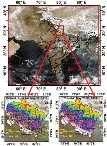
Figure 2. Methodology implemented in the WRF-Chem model simulations for this study.

3. Results

3.1. Event-1: 24 April to 2 May 2016

In the year 2016, limited rainfall was received over Uttarakhand during winter, which made it abnormally warm and lead to loss of moisture from soil and air (Thakur et al. 2019). This dry atmospheric condition resulted in huge amount of dry litter and vegetation fuel over forest covered areas of Uttarakhand. These favorable conditions triggered a widespread forest fire over Uttarakhand during April–May 2016 (Negi 2016). Total burnt area was estimated to be 3774.1 km² (15.3% of the total forest cover of the Uttarakhand) with total active forest fires of ~1600 over Uttarakhand during 24 April 24 to 2 May 2016 (Jha et al. 2016; Gupta et al. 2018). The most affected districts were Tehri Garhwal, Pauri Garhwal, Nainital, Almora, Bageshwar, and Champawat (Gupta et al. 2018). This event introduced enormous amount of pollutants in the pristine atmosphere of Uttarakhand. Distribution of gaseous pollutants like NOx, CO, and O₃ are studied over fire affected region during this event.

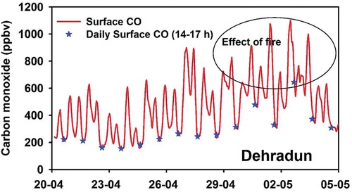
Figure 3 shows 4 h moving average CO variation from 20 April to 5 May 2016 over Dehradun. The typical urban diurnal variation of CO (morning and evening peaks) was observed throughout the study period. However, the diurnal baseline of CO mixing ratio (values during 14–17 h) started increasing from 24th April onwards. To evaluate the rate of increase of CO due to BB emission, daily noon hour (14–17 h) average CO mixing ratio was investigated. This time period was chosen because CO showed minimum value during this period of the day. Daily noon hour averaged CO or daily baseline CO showed systematic increase (29 ppbv/day) from 24 April to 1 May. The fire activities were maximum during this period which confirmed the addition of excess CO in daily CO level.

Figure 3. Temporal variation of surface CO (4 h moving average) and daily 14–17 h average surface CO over Dehradun during 20 April to 5 May 2016.

3.2. Impact of biomass burning on trace gases during event-1

To estimate the pollution enhancement due to forest fire episode, WRF-Chem model simulations were made over the study region with two different emission scenarios: one with BB emissions and another without BB emissions.

Figure 4. Average simulated spatial distribution of NOx, CO, and O₃ at surface, with BB emissions (top panel) and without BB emissions (bottom panel) in the domain d02 during 30 April to 1 May 2016 (peak period of forest fire). The black circle shows the location of observational site. Average WRF-Chem simulated surface wind vectors are also overlaid on each plot.

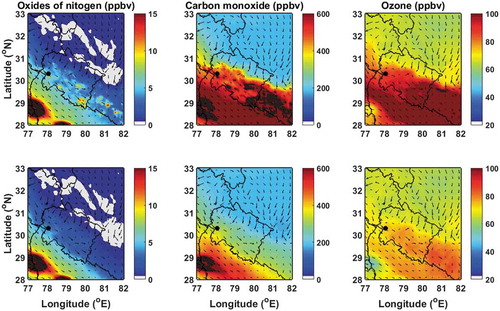
The average spatial distribution of surface NOx, CO, and O₃ simulated by WRF-Chem with BB emissions (top panel) and without BB emissions (bottom panel) are shown in Figure 4. Model simulated wind vectors are also overlaid in these figures. The spatial distribution showed significant increase of CO and O₃ levels specifically over south and south-eastern parts of Uttarakhand. The enhanced concentrations were estimated up to 300 ppbv, 20 ppbv, and 5 ppbv for CO, O₃, and NOx, respectively over this region. The NOx distribution showed high values close to fire hotspots due to shorter life time. The wind vectors showed that north-westerly winds prevailed over the fire affected region during this period. These winds might have transported fire plume toward downwind locations. This has been examined using HYSPLIT (Hybrid Single particle Lagrangian Integrated Trajectory) model (http://www.arl.noaa.gov/ready.html) (Rolph, Stein, and Stunder 2017). The 48 h ensemble forward trajectories were computed over fire affected regions of Uttarakhand at an altitude of 500 m during peak fire period. The forward-trajectory analysis showed that the fire plumes were transported toward Nepal and Indo Gangetic Plain (IGP). The height of trajectories was found to be mostly lower than 3 km over the downwind regions. Thus, fire plume might have influenced the air quality over these regions.

Figure 5. Time series of simulated mixing ratios (ppbv) of CO, O₃, and NOx with BB emissions (Mod-BB), without BB emissions (Mod-NoBB), and their percentage difference (%) during 20 April to 5 May 2016 over Dehradun. Top panel also shows in-situ observation of CO over Dehradun. Bottom panel shows daily fire counts over Uttarakhand.

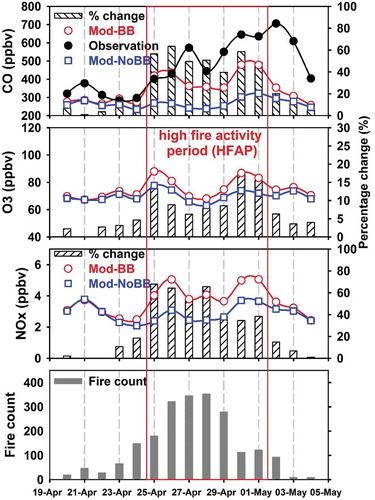
Figure 5 shows daily WRF-Chem simulated CO, O₃, and NOx under two emission scenarios (with and without BB) along with in-situ observations over Dehradun for 20 April to 4 May 2016. Bottom panel of this figure shows total number of fire hotspots over Uttarakhand obtained from MODIS (Moderate Resolution Imaging Spectroradiometer). The MODIS fire counts indicate that fire activity exacerbated on 24 April onwards, peaked during 26 April to 28 April and diminished afterward. A high fire activity period (HFAP) is defined based on MODIS fire counts to study the influence of this fire episode on the air quality over Uttarakhand. HFAP is defined when three days running mean of MODIS fire counts exceeds the median fire counts during the study period (Kumar et al. 2011; Piyush et al. 2018). The HFAP period is identified from 25 April to 1 May for Event-1.

Figure 6. (a) Scatter plot between change in CO (∆CO) and change in O₃ (∆O₃) at surface. (b) Daily variation of enhancement ratio (∆O₃/∆CO) during study period over Dehradun.

Top panel of Figure 5 shows comparison of CO obtained from in-situ observations and model simulations. Before HFAP, model showed only slight underestimation of CO over Dehradun. However, during and after HFAP, the difference between observed and simulated CO was found to be large (45–350 ppbv). Top three panels of Figure 5 represent the daily variations of CO, O₃ and NOx simulated by WRF-Chem with and without BB emissions along with their absolute percentage difference [100*(Mod-BB minus Mod-NoBB)/Mod-NoBB)]. Model showed a considerable increase in CO mixing ratio upto 177 ppbv, NOx levels upto 2 ppbv and O₃ levels upto 13 ppbv due to fire event. During HFAP, the CO mixing ratios enhanced by 40–63% with average of 52%, NOx mixing ratios enhanced by 35–68% with average of 52%, whereas O₃ mixing ratios enhanced by 6–18% with average of 11%.

In order to measure the ozone production in air mases originated from BB sources, we calculated enhancement ratio from WRF-Chem simulations. Enhancement ratio is defined as excess O₃ mixing ratio due to a particular source as a function of increased CO from the same source, i.e. forest fires. It can be helpful to estimate the increased production of O₃ due to BB as a function of increased CO emissions from the same source (Parrish et al. 1993; Pfister et al. 2006; Thomas et al. 2013). Enhancement ratio depends on many parameters like model resolution, plume rise transport, uncertainties in the fire emissions, etc. However, the assessment of these parameters was beyond the scope of this research paper. We calculated ∆O₃ (O_{3 with BB} minus O_{3 without BB}) and ∆CO (CO_{with BB} minus CO_{without BB}) from the model simulations. Subsequently, we calculated the enhancement ratios (∆O₃/∆CO) in fire plume during the study period over Dehradun. Change in O₃ (∆O₃) with change in CO (∆CO) at surface and daily variation of enhancement ratios (∆O₃/∆CO) are shown in Figure 6(a) and (b), respectively during the study period. A clear positive correlation of 0.89 was found between ∆O₃ and ∆CO. This indicates that the excess O₃ was produced due to photo-chemistry of its precursors emitted from BB. The similar correlation was found over North eastern India and Myanmar region during spring (March–May) 2005 (Jena et al. 2015). The average enhancement ratio (∆O₃/∆CO) was found to be 0.08 ppbv/ppbv during study period over Dehradun.

Figure 7. Time verses pressure of daily average vertical distribution of ∆CO, ∆NOx, and ∆O₃ during 20 April to 4 May 2016.

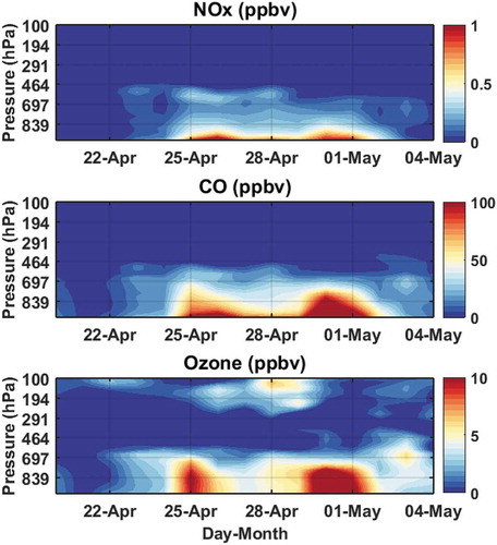
The emissions of trace gases are released close to the Earth’s surface. The vertical mixing/atmospheric boundary layer dynamics can transport the emitted species deeper in the atmosphere. In order to investigate the vertical mixing of BB plume during Event-1, the vertical variation of daily averaged ∆NOx, ∆CO, and ∆O₃ were examined over Dehradun (Figure 7). The increased amount of these gases due to fire episode clearly persisted during HFAP and dissipated afterward. An interesting bimodal variation was observed in the temporal distribution of ∆NOx, ∆CO, and ∆O₃. Their vertical variations showed two peaks on 25 and 30 April 2016. This may be due to dispersion and mixing of forest fire plume with the air of nearby locations. The influence of these processes may differ from one day to other resulting in uneven increase of air pollutants over Dehradun. The absolute change in the concentration of these species gradually decreased toward higher altitudes up to 6.5 km (450 hPa). The average change of CO (O₃) decreased significantly from 142 ± 29 ppbv (8 ± 3 ppbv) at surface to 10 ± 8 ppbv (0.3 ± 0.5 ppbv) at 5 km (550 hPa) during HFAP. The NOx concentration decreased rapidly from surface to higher altitudes with 1.5 ± 0.3 ppbv at surface and 0.1 ± 0.1 ppbv at 5 km.

3.3. Event-2: 20–30 May 2018

Forest fires in the year 2016 set an alarm for need of strict control measures for these events. But despite getting highlighted in news, research articles and reports, the forest fire again occurred in 2018. Similar to Event-1, widespread fire occurred over Uttarakhand during 17–31 May 2018. The districts that had the highest proportion of burnt area were Pauri Garhwal, Almora, Bageshwar, Uttarkashi, and Tehri. The main forest type which caught fire was Chir pine forest, with 390.8 km² burnt area followed by dry deciduous scrub with 177.2 km² burnt area.

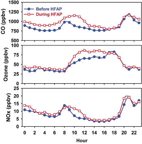
These fires caused degradation of air quality over Uttarakhand. Gaseous air pollutants like ozone, NO_X, and CO again showed enhanced levels during this fire event. The HFAP period is defined according to method described in Section 3.2 and is identified as 20–30 May for Event-2. Figure 8 shows the diurnal variation of CO, ozone, and NOx before HFAP (17–19 May) and during HFAP. Like CO, diurnal variation of NOx showed typical urban pattern over Dehradun with daily morning and late evening peaks. These peaks were attributed to combinations of anthropogenic activities, chemistry, and boundary layer dynamics. The daily values of NOx and CO were enhanced significantly upto 5 ppbv (up to 87%) and 270 ppbv (up to 32%), respectively during HFAP. Ozone showed broad peak during daytime (10–16 h) due to its photochemical production from its precursors (CO, NO_x, etc.). Daily daytime average ozone increased by 17 ppbv (approximately 27%) during HFAP.

Figure 8. Diurnal variation of surface CO, O₃, and NOx before HFAP (17–19 May) and during HFAP (20–30 May 2018) over Dehradun.

3.4. Impact of biomass burning on trace gases during event-2

Figure 9 shows the spatial distribution of simulated surface concentration of NOx, CO, and O₃ with BB emissions (top panel) and without BB emissions (bottom panel), along with average surface wind vectors during 21–22 May 2018. The spatial distribution showed clear increase of NOx, CO, and O₃ levels over southern region of Uttarakhand. The enhanced concentrations of NOx, CO, and O₃ were mostly confined to the fire hotspot regions of Uttarakhand as depicted in Figure 1(b). The horizontal wind vectors overlaid on Figure 9 showed relatively lower wind speed during Event-2 as compared to Event-1. Wind was found to be north-westerly over the source region. The 48 h HYSPLIT forward trajectories were computed for three locations at an altitude of 500 m representing western, central, and eastern parts of Uttarakhand during HFAP (not shown). The forward-trajectory analysis showed that the fire impacted plumes were transported toward Nepal and IGP similar to Event-1.

Figure 9. Average simulated spatial distribution of NOx, CO, and O₃ at surface, with BB emissions (top panel) and without BB emissions (bottom panel) in the domain d02 during 21–22 May 2018 (peak period of forest fires). The black circle shows the location of observational site IIRS, Dehradun. Average WRF-Chem simulated surface wind vectors are also overlaid on each plot.

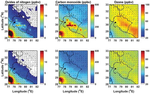
Figure 10 shows the daily variation of observed and simulated concentrations of CO, O₃, and NOx over Dehradun along with daily fire counts over Uttarakhand during 17–31 May 2018. Fire activity started from 20th May onwards and peaked on 22 May. MODIS showed maximum fire counts of 164 over Uttarakhand on that day. The observed CO mixing ratio increased from 21 May onwards, attained maximum on 28 May and subsequently decreased. The rate of increase of CO was 9 ppbv/day while it was very small for NOx and O₃ during the study period (May 17–31). The average mixing ratios of NOx, CO, and O₃ were 10 ± 1 ppbv, 946 ± 78 ppbv, and 55 ± 9 ppbv, respectively during entire study period, whereas 10 ± 1 ppbv, 974 ± 73 ppbv, and 58 ± 8 ppbv, respectively during HFAP.

Figure 10. Time series of simulated mixing ratios (ppbv) of CO, O₃, and NOx with BB emission (Mod-BB), without BB emission (Mod-NoBB), their percentage difference (%) along with their observational values during 17–31 May 2018 over Dehradun. Bottom panel shows daily fire counts over Uttarakhand.

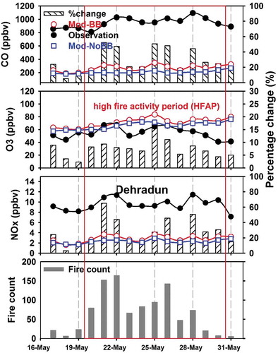
Figure 10 also represents the daily variations of CO, O₃, and NOx simulated by WRF-Chem with, without fire emissions along with their absolute percentage difference during study period. Due to fire event, the enhancements were estimated upto 118 ppbv, 1 ppbv, and 12 ppbv for CO, NOx, and O₃, respectively during the study period. During HFAP, the CO levels enhanced by 18–52% with average of 34%, NOx enhanced by 14–65% with average of 32% while slight enhancement of O₃ levels by 4–17% with average of 9%. These enhanced mixing ratios were relatively lower as compared to Event-1, which may be attributed to lower intensity of forest fire during Event-2. The fire burnt area was estimated as 690.8 km² area, which was 2.8% of the total forest area of Uttarakhand. This was much less as compared to Event-1 where the burnt area was estimated as 15.3% (Gupta et al. 2018).

Figure 11. (a) Scatter plot between change in CO (∆CO) and change in O₃ (∆O₃) at surface. (b) Daily variation of enhancement ratio (∆O₃/∆CO) during study period over Dehradun.

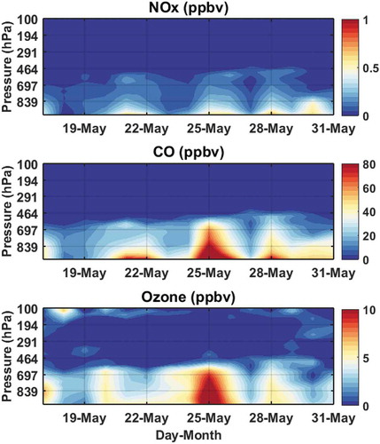
Figure 12. Time verses pressure of daily average vertical distribution of ∆CO, ∆NOx, and ∆O₃ during 17–31 May 2018.

Correlation between change in O₃ (∆O₃) with change in CO (∆CO) at surface and daily variation of enhancement ratios (∆O₃/∆CO) are shown in the Figure 11(a,b), respectively during the study period. The correlation coefficient between ∆O₃ and ∆CO was estimated to be 0.69 and the average of enhancement ratio (∆O₃/∆CO) was found to be 0.09 ppbv/ppbv during this event. This indicates that excess O₃ produced due to photo-chemistry of its precursors emitted during this event. Correlation and average enhancement ratio for this event is comparable with Event-1 and agrees well with other studies (Mauzerall et al. 1998; Takegawa et al. 2003; Singh et al. 2010; Jena et al. 2015).

The vertical distribution of daily averaged enhancements of trace gases (∆NOx, ∆CO, and ∆O₃) were examined during Event-2 over Dehradun (Figure 12). The vertical mixing of fire plume was clearly evident on the vertical distribution of these gases. The impact of convection was specifically observed on the vertical distribution of ∆CO and ∆O₃ on 25 May 2018 but not in ∆NOx concentration due to smaller lifetime of NOx in the lower troposphere. During HFAP, the absolute change in the concentration of these species was gradually decreasing toward higher altitudes (upto 6.5 km). The average change of CO (O₃) decreased significantly from 72 ± 31 ppbv (6 ± 2 ppbv) at surface to 11 ± 8 ppbv (1 ± 1 ppbv) at 5 km during HFAP. The NOx concentration decreased rapidly from surface to higher altitudes as it was 0.6 ± 0.3 ppbv at surface and 0.1 ± 0.1 ppbv at 5 km. The ∆CO and ∆NOx variations again showed alternate high and low value days indicating the role of mixing and dispersion of fire plume.

4. Discussion

4.1. Uncertainty in biomass burning emissions

The quantitative estimation of CO, NOx, and O₃ enhancement due to BB emissions may contain uncertainties related to BB emission estimates (Wiedinmyer et al. 2011). The accuracy of FINN BB emissions used in the present study depends on the active fire products obtained from MODIS, accuracy of LULC classifications, fuel loading and consumption, uncertainties in EFs, etc. MODIS underestimates the fire counts as compared to other advanced satellite-based instruments like Visible Infrared Imaging Radiometer Suite (VIIRS) (Giglio et al. 2010; Vadrevu and Lasko 2018). Vadrevu and Lasko (2018) compared fire counts and fire radiative power (FRP) obtained from MODIS and VIIRS. The VIIRS fire counts were found to be higher by a factor of 4.8 times and FRP higher by a factor of 2.5 times with respect to MODIS. Most resent BB emission inventories like GFED (Global Fire Emission Database) and FINN still use MODIS fire products for derivation of BB emissions that may cause underestimation of air pollutants in model simulation.

Typically, higher emissions are estimated for forests than grasslands due to the variable fuel loadings. Thus, classification of land cover and vegetation type can introduce significant amount error in the emission estimates. Wiedinmyer et al. (2006) reported that the use of different LULC datasets to estimate regional fire emissions led to 26% difference in the estimation of annual emissions for North and Central America. For example, the GLOBCOVER assigned 70% more forest fires to the contiguous U.S., Mexico, and Central America with respect to MODIS LCT (Land Cover Type). Utilization of this dataset lead to 20% and 24% higher CO and NMVOC emissions respectively with respect to MODIS LCT simulation over these regions (Wiedinmyer et al. 2011). In addition, uncertainties may also arise in the annual variation of EFs. The EFs measured in 2011 differed by ∼13–195% as compared EFs measured in 2010 over south-eastern US (Akagi et al. 2013).

Mieville et al. (2010) reported 15–50% uncertainty in the available BB emissions for different species. Thomas et al. (2013) showed that emissions of CO and NMHCs were too low while emissions of NOx were high in the FINN inventory. Researchers reported that two-fold increase of CO emissions (2xCO) from fires in the model simulation can provide a better agreement with observations (Thomas et al. 2013; Cuchiara et al. 2017).

4.2. Comparison with other model studies

BB is one of the most important sources of air pollution on our Earth. Several modeling attempts have been made to quantify the contribution of BB in the air pollution enhancement all over the globe. Cuchiara et al. (2017) investigated the impact of widespread forest fire event occurred over South America during summer 2014 on the ozone distribution using WRF-Chem. Ozone levels enhanced due to this event up to 10 ppbv. Sensitivity simulations of model showed that an increase in BB emissions by 4 and 8 times can enhance the ozone levels upto 10–15 ppbv and 20–25 ppbv, respectively. Srivastava and Sheel (2013) used MOZART-4 (global CTM) to simulate the vertical distribution of ozone and CO over Indonesia during an intense biomass burring event in autumn 2006. Model simulation with and without BB emissions revealed the enhancement of CO by 104 ± 56 ppbv and O₃ by 5 ± 1 ppbv from surface to 100 hPa over Indonesia due to this fire episode. Thomas et al. (2013) used regional and global models to simulate the ozone distribution over Greenland in summer 2008. The sensitivity simulations showed upto 5% (3 ppbv) enhancement in ozone due to BB. Jena et al. (2015) demonstrated impact of BB emissions on surface concentrations of CO, NO₂, and O₃ over south-east Asia during spring 2005 using WRF-Chem sensitivity simulations. They showed that surface concentrations of CO and NO₂ were increased by 35–60% and surface levels of O₃ was increased by 25–40% over eastern region of India including Myanmar due to BB emissions. However, these efforts particularly lack over fire prone Uttarakhand region situated in the foothills of north western Himalaya. In the present work, the WRF-Chem model simulations are used in nested domain mode to quantify the enhanced concentration of CO, O₃, and NOx at very fine horizontal resolution (9 km × 9 km) due to BB events over Uttarakhand. The enhanced concentrations are estimated up to 300 ppbv, 20 ppbv, and 5 ppbv for CO, O₃, and NOx, respectively over this region during these events. These results are consistent with previous studies.

The two simulations made with and without BB emissions have been used to quantify the production of ozone due to fire emissions. Enhancement ratio (∆O₃/∆CO), change in concentration of ozone with respect to change in concentration of CO due to BB, was calculated and compared with values reported in previous studies (Table 2). The enhancement ratio was estimated to be 0.08 and 0.09 ppbv/ppbv for these events during 2016 and 2018, respectively over Dehradun. This agrees well with ratio of 0.10 over Canada during June–July (Mckeen et al. 2002), 0.12 ppbv/ppbv over Australia during August–September and 0.12 ppbv/ppbv over North eastern India and Myanmar region during spring (Takegawa et al. 2003; Jena et al. 2015). A little higher average enhancement ratio of 0.15 ppbv/ppbv was estimated over NE Pacific/NW United States during August, 2003 (Bertschi and Jaffe 2005).

Table 2. Enhancement ratios (∆O₃/∆CO) of present study (Event-1 and Event-2) and from the previous studies.

Region	Date	Enhancement Ratio (ppbv/ppbv)	Reference
Canada	June–July 1995	0.10	Mckeen et al. (2002)
Australia	August–September 1999	0.12	Takegawa et al. (2003)
NE Pacific/NW United States	August 2003	0.15	Bertschi and Jaffe (2005)
North eastern India and Myanmar, South-East Asia	March–May 2005	0.12	Jena et al. (2015)
Dehradun, Uttarakhand	Event-1, 2016	0.08	This study
Dehradun, Uttarakhand	Event-2, 2018	0.09	This study

4. Summary and conclusions

Influence of two forest fire events was analyzed on the distribution of ozone, CO, and NOx distribution over Uttarakhand, India using in-situ observations and WRF-Chem simulations. These events occurred during 24 April to 2 May 2016 (Event-1) and 20–30 May 2018 (Event-2). The burnt area was estimated as 3774.14 km² (15.3% of total forested area of Uttarakhand) for Event-1 and 690.8 km² (2.8% of total forested area of Uttarakhand) for Event-2. Approximately, 448.1 km² forest area experienced fire in both the years 2016 and 2018, i.e. 64.87% of the burnt area of year 2018 had fire in the year 2016 also. This can be deduced that these areas of Uttarakhand are more prone to forest fire. These events injected a lot of air pollutants like NOx, CO, and O₃ in the clean atmosphere of Uttarakhand. For Event-1, the spatial distribution showed significant increase of CO and O₃ levels specifically over south and south-eastern parts of Uttarakhand. The enhanced concentrations are estimated up to 300 ppbv, 20 ppbv, and 5 ppbv for CO, O₃, and NOx, respectively over this region. During this period, the wind was found to be north-westerly over the study region. These winds might have transported polluted air toward Nepal and IGP regions. For Event-2, the spatial distribution showed clear increase of NOx, CO, and O₃ levels over southern region of Uttarakhand. The enhanced concentrations of NOx, CO, and O₃ were mostly confined to the fire hotspot regions. During HFAP, wind pattern was again north-westerly specifically over the source regions.

The major findings of present work are summarized below

• During Event 1, the observed CO mixing ratio over Dehradun increased from 25 April onwards, attained maximum (705.8 ± 258 ppbv) on 2 May 2016 and subsequently decreased. The rate of increase of daily baseline CO was 29 ppbv/day during HFAP (24 April 24 to 1 May 2016).

• For Event-1, WRF-Chem simulation showed 52% enhancement in CO, 52% enhancement in NOx and 11% enhancement in O₃ during HFAP. A clear positive correlation (r = 0.89) was observed between ∆O₃ (O_{3 with BB} minus O_{3 without BB}) and ∆CO (CO_{with BB} minus CO_{without BB}) indicating rapid production of ozone in the fire plume. The average enhancement ratio (∆O₃/∆CO) was found to be 0.08 ppbv/ppbv during this event.

• During Event-1 and Event-2, the spatial distribution showed clear increase in NOx, CO, and O₃ levels over fire affected regions of Uttarakhand.

• Daily variation of observed concentrations of CO, O₃, and NOx showed influence of forest fires during 20–30 May 2018 over Dehradun. The rate of increase of CO was 9 ppbv/day while it was very small for NOx and O₃ during HFAP period.

• During HFAP, WRF-Chem simulated CO and NOx levels enhanced significantly by 34% and 32%, respectively while O₃ levels enhanced by 9%. A good correlation (r = 0.69) was observed between ∆O₃ and ∆CO indicating photochemical production of ozone in the fire plumes.

• The vertical distribution of ∆O₃, ∆CO, and ∆NOx showed that forest fire events influenced the air quality up to 6.5 km in altitude.

Wind pattern over Uttarakhand is mostly westerly/north-westerly except monsoon season. The north/north eastern parts of Uttarakhand are snow covered high altitude mountains, which prevent the northward movement of fire plume. Pertaining to wind pattern, the most probable path for fire plume is its transport toward IGP. This is world’s most densely populated region (500–1000 or more persons/km², based on 2001 census) situated between Himalayan mountains in North and Deccan Plateau in south. This geographical structure is not favorable for dispersion of polluted air. Thus, severe forest fires in the dense forest of foothills of north-western Himalaya can severely influence the air quality of this highly populated region. Therefore, forest fire events in this area and their influence over the downwind regions should be investigated in detail using in-situ, satellite, and modeling-based approach to make the necessary policies and avoid the possible health consequences.

Acknowledgements

The present study is supported by ISRO-Geosphere Biosphere Program. We are thankful to the teams of MODIS, NCEP reanalysis data and MOZART for providing the respective data sets. We are also grateful to Director IIRS, Dr. Prakash Chauhan and Dean IIRS, Dr. S.K. Srivastava for their encouragement and support. We are thankful to anonymous reviewers for their constructive suggestions and insightful comments which have improved the quality of this manuscript significantly.

Disclosure statement

No potential conflict of interest was reported by the authors.

Additional information

Funding

This work was supported by ISRO-Geosphere Biosphere Program.

References

- Abushenko, N. A., D. A. Altyntsev, A. A. Muzurov, and N. P. Min’ko. 2000. “AVHRR/NOAA Data in Estmating Areas of Large Forest Fires.” Mapping Sciences & Remote Sensing 37 (3): 180–188. doi:10.1080/07493878.2000.10642147.
- Akagi, S. K., R. J. Yokelson, I. R. Burling, S. Meinardi, I. Simpson, D. R. Blake, G. R. McMeeking, et al. 2013. “Measurements of Reactive Trace Gases and Variable O3 Formation Rates in Some South Carolina Biomass Burning Plumes.” Atmospheric Chemistry and Physics 13 (3): 1141–1165. doi:10.5194/acp-13-1141-2013.
- Al-Saadi, J., A. Soja, R. B. Pierce, J. Szykman, C. Wiedinmyer, L. Emmons, S. Kondragunta, et al. 2008. “Intercomparison of Near-real-time Biomass Burning Emissions Estimates Constrained by Satellite Fire Data.” Journal of Applied Remote Sensing 2 (1): 21504. doi:10.1117/1.2948785.
- Andreae, M. O., and P. Merlet. 2001. “Emission of Trace Gases and Aerosols from Biomass Burning.” Global Biogeochemical Cycles 15 (4): 955–966. doi:10.1029/2000GB001382.
- Arino, O., P. Bicheron, F. Achard, J. Latham, R. Witt, and J. L. Weber. 2008. “GlobCover: The Most Detailed Portrait of Earth.” Europe Sp Agency Bulletin (2008) (136): 24–31.
- Bahuguna, V. K., and A. Upadhay. 2002. “Forest Fires in India: Policy Initiatives for Community Participation.” International For Reverend 4 (2): 122–127. doi:10.1505/ifor.4.2.122.17446.
- Bartholomé, E., and A. S. Belward. 2005. “GLC2000: A New Approach to Global Land Cover Mapping from Earth Observation Data.” International Journal of Remote Sensing 26 (9): 1959–1977. doi:10.1080/01431160412331291297.
- Beig, G., S. Gunthe, and D. B. Jadhav 2007. Simultaneous measurements of ozone and its precursors on a diurnal scale at a semi urban site in India, Journal of Atmospheric Chemistry, doi:10.1007/s10874-007-9068-8.
- Bertschi, I. T., and D. A. Jaffe. 2005. “Long-range Transport of Ozone, Carbon Monoxide, and Aerosols to the NE Pacific Troposphere during the Summer of 2003.” Observations of Smoke Plumes from Asian Boreal Fires 110: 1–15. doi:10.1029/2004JD005135.
- Calle, A., P. Salvador, and F. González-Alonso. 2013. “Study of the Impact of Wildfire Emissions, through MOPITT Total CO Column, at Different Spatial Scales.” International Journal of Remote Sensing 34 (9–10): 3397–3415. doi:10.1080/01431161.2012.716534.
- Chand, K. T. R., K. V. S. Badarinath, M. S. R. Murthy, G. Rajshekhar, C. D. Elvidge, and B. T. Tuttle. 2007. “Active Forest Fire Monitoring in Uttaranchal State, India Using Multi-temporal DMSP-OLS and MODIS Data.” International Journal of Remote Sensing 28 (10): 2123–2132. doi:10.1080/01431160600810609.
- Chen, F., and J. Dudhia. 2001. “Coupling an Advanced Land-surface-hydrol- Ogy Model with Penn state-NCAR MM5 Modeling System, Part I: Model Implementation and Sensitivity.” Monthly Weather Review, no. 129: 569–585. doi:10.1175/1520-0493(2001)129<0569:CAALSH>2.0.CO;2.
- Crutzen, P. J., and M. O. Andreae. 1990. “Biomass Burning in the Tropics: Impact on Atmospheric Chemistry and Biogeochemical Cycles.” Science 250 (4988): 1669–1678. doi:10.1126/science.250.4988.1669.
- Cuchiara, G. C., B. Rappenglück, M. A. Rubio, E. Lissi, E. Gramsch, and R. D. Garreaud. 2017. “Modeling Study of Biomass Burning Plumes and Their Impact on Urban Air Quality; a Case Study of Santiago De Chile.” Atmospheric Environment 166: 79–91. doi:10.1016/j.atmosenv.2017.07.002.
- Deep, A., C. P. Pandey, H. Nandan, K. D. Purohit, N. Singh, J. Singh, A. K. Srivastava, and N. Ojha. 2019. “Evaluation of Ambient Air Quality in Dehradun City during 2011–2014.” Journal of Earth System Science 128 (4). doi:10.1007/s12040-019-1092-y.
- Duncan, B. N. 2003. “Indonesian Wildfires of 1997: Impact on Tropospheric Chemistry.” Journal of Geophysical Research 108 (D15): 4458. doi:10.1029/2002JD003195.
- Emmons, L. K., S. Walters, P. G. Hess, J.-F. Lamarque, G. G. Pfister, D. Fillmore, C. Granier, et al. 2010. “Description and Evaluation of the Model for Ozone and Related Chemical Tracers, Version 4 (MOZART-4).” Geoscientific Model Development 3 (1): 43–67. doi:10.5194/gmd-3-43-2010.
- Friedl, M. A., D. K. McIver, J. C. F. Hodges, X. Y. Zhang, D. Muchoney, A. H. Strahler, C. E. Woodcock, et al. 2002. “Global Land Cover Mapping from MODIS: Algorithms and Early Results.” Remote Sensing of Environment 83 (1–2): 287–302. doi:10.1016/S0034-4257(02)00078-0.
- Ghude, S. D., S. Fadnavis, G. Beig, S. D. Polade, and R. J. van der A. 2008. “Detection of Surface Emission Hot Spots, Trends, and Seasonal Cycle from Satellite-retrieved NO2 over India.” Journal of Geophysical Research 113 (D20): 1–13. doi:10.1029/2007JD009615.
- Giglio, L., J. T. Randerson, G. R. Van Der Werf, P. S. Kasibhatla, G. J. Collatz, D. C. Morton, and R. S. Defries. 2010. “Assessing Variability and Long-term Trends in Burned Area by Merging Multiple Satellite Fire Products.” Biogeosciences 7 (3): 1171–1186. doi:10.5194/bg-7-1171-2010.
- Gleason, C., and J. Im. 2011. “A Review of Remote Sensing of Forest Biomass and Biofuel: Options for Small-area Applications.” GIScience & Remote Sensing 48 (2): 141–170. doi:10.2747/1548-1603.48.2.141.
- Granier, C., B. Bessagnet, T. Bond, A. D’Angiola, H. D. van der Gon, G. J. Frost, A. Heil, et al. 2011. “Evolution of Anthropogenic and Biomass Burning Emissions of Air Pollutants at Global and Regional Scales during the 1980–2010 Period.” Climatic Change 109 (1–2): 163–190. doi:10.1007/s10584-011-0154-1.
- Grell, G. A., and S. R. Freitas. 2014. “A Scale and Aerosol Aware Stochastic Convective Parameterization for Weather and Air Quality Modeling.” Atmospheric Chemistry and Physics 14 (10): 5233–5250. doi:10.5194/acp-14-5233-2014.
- Grell, G. A., R. Knoche, S. E. Peckham, and S. A. McKeen. 2004. “Online versus Offline Air Quality Modeling on Cloud-resolving Scales.” Geophysical Research Letters 31 (April): 6–9. doi:10.1029/2004GL020175.
- Guenther, A., T. Karl, P. Harley, C. Wiedinmyer, P. I. Palmer, and C. Geron. 2006. “Estimates of Global Terrestrial Isoprene Emissions Using MEGAN (Model of Emissions of Gases and Aerosols from Nature).” Atmospheric Chemistry and Physics 6 (1): 107–173. doi:10.5194/acpd-6-107-2006.
- Gupta, S., A. Roy, D. Bhavsar, R. Kala, S. Singh, and A. S. Kumar. 2018. “Forest Fire Burnt Area Assessment in the Biodiversity Rich Regions Using Geospatial Technology: Uttarakhand Forest Fire Event 2016.” Journal of the Indian Society of Remote Sensing 46 (6): 945–955. doi:10.1007/s12524-018-0757-3.
- Hansen, M. C., R. S. DeFries, J. R. G. Townshend, R. Sohlberg, C. Dimiceli, and M. Carroll. 2002. “Towards an Operational MODIS Continuous Field of Percent Tree Cover Algorithm: Examples Using AVHRR and MODIS Data.” Remote Sensing of Environment 83 (1–2): 303–319. doi:10.1016/S0034-4257(02)00079-2.
- Hashim, M., K. D. Kanniah, A. Ahmad, A. W. Rasib, and A. L. Ibrahim. 2004. “The Use of AVHRR Data to Determine the Concentration of Visible and Invisible Tropospheric Pollutants Originating from a 1997 Forest Fire in Southeast Asia.” International Journal of Remote Sensing 25 (21): 4781–4794. doi:10.1080/01431160410001712963.
- Hong, S. Y., Y. Noh, and J. Dudhia. 2006. “A New Vertical Diffusion Package with an Explicit Treatment of Entrainment Processes.” Monthly Weather Review 134: 2318–2341. doi:10.1175/MWR3199.1.
- Iacono, M. J., J. S. Delamere, E. J. Mlawer, M. W. Shephard, S. A. Clough, and W. D. Collins. 2008. “Radiative Forcing by Long-lived Greenhouse Gases: Calculations with the AER Radiative Transfer Models.” Journal of Geophysical Research 113: (D13). doi:10.1029/2008JD009944.
- Ichoku, C., R. Kahn, and M. Chin. 2012. “Satellite Contributions to the Quantitative Characterization of Biomass Burning for Climate Modeling.” Atmospheric Research 111: 1–28. doi:10.1016/j.atmosres.2012.03.007.
- Janjic, Z. I. 1996. “The Surface Layer in the NCEP Eta Model.” In Eleventh Con- ference on Numerical Weather Prediction, Norfolk, VA, 19–23 August, 354–355. Boston, MA: American Meteorological Society.
- Jena, C., S. D. Ghude, G. G. Pfister, D. M. Chate, R. Kumar, G. Beig, D. E. Surendran, S. Fadnavis, and D. M. Lal. 2015. “Influence of Springtime Biomass Burning in South Asia on Regional Ozone (O3): A Model Based Case Study.” Atmospheric Environment 100: 37–47. doi:10.1016/j.atmosenv.2014.10.027.
- Jha, C. S., R. Gopalakrishnan, K. C. Thumaty, J. Singhal, C. S. Reddy, J. Singh, S. V. Pasha, et al. 2016. “Monitoring of Forest Fires from Space – ISRO ’ S Initiative for near Real-time Monitoring of the Recent Forest Fires in Uttarakhand, India.” Current Science 110 (11): 2057–2060. D. V.
- Karathanassi, V., V. Andronis, and D. Rokos. 2003. “The Radiative Impact of Aerosols Emanating from Biomass Burning, through the Minnaert Constant.” International Journal of Remote Sensing 24 (24): 5135–5145. doi:10.1080/0143116031000080750.
- Kondo, Y., Morino, Y., Takegawa, N., Koike, M., Kita, K., Miyazaki, Y., Sachse, G.W., Vay, et al. 2004. “Impacts of biomass burning in Southeast Asia on ozone and reactive nitrogen over the western Pacific in spring”. Journal of Geophysical Research 109. doi:10.1029/2003JD004203
- Kumar, R., M. Naja, S. K. Satheesh, N. Ojha, H. Joshi, T. Sarangi, P. Pant, U. C. Dumka, P. Hegde, and S. Venkataramani. 2011. “Influences of the Springtime Northern Indian Biomass Burning over the Central Himalayas.” Journal of Geophysical Research 116 (D19): 302. doi:10.1029/2010JD015509.
- Lamarque, J.-F., T. C. Bond, V. Eyring, C. Granier, A. Heil, Z. Klimont, D. Lee, et al. 2010. “Historical (1850–2000) Gridded Anthropogenic and Biomass Burning Emissions of Reactive Gases and Aerosols: Methodology and Application.” Atmospheric Chemistry and Physics 10 (15): 7017–7039. doi:10.5194/acp-10-7017-2010.
- Lei, W., G. Li, and L. T. Molina. 2013. “Modeling the Impacts of Biomass Burning on Air Quality in and around Mexico City.” Atmospheric Chemistry and Physics 13 (5): 2299–2319. doi:10.5194/acp-13-2299-2013.
- Lin, Y. L., R. D. Farley, and H. D. Orville. 1983. “Bulk Parameterization of the Snow Field in a Cloud Model.” Journal of Climate and Applied Meteorology 22 (6): 1065–1092. doi:10.1175/1520-0450(1983)022<1065:BPOTSF>2.0.CO;2.
- Lu, Z., Q. Zhang, and D. G. Streets. 2011. “Sulfur Dioxide and Primary Carbonaceous Aerosol Emissions in China and India, 1996-2010.” Atmospheric Chemistry and Physics 11 (18): 9839–9864. doi:10.5194/acp-11-9839-2011.
- Marlier, M. E., R. S. Defries, P. S. Kim, D. L. A. Gaveau, S. N. Koplitz, D. J. Jacob, L. J. Mickley, B. A. Margono, and S. S. Myers. 2015. “Regional Air Quality Impacts of Future Fire Emissions in Sumatra and Kalimantan.” Environmental Research Letters 10 (5): 054010. doi:10.1088/1748-9326/10/5/054010.
- Mauzerall, D. L., J. A. Logan, D. J. Jacob, B. E. Anderson, D. R. Blake, J. D. Bradshaw, B. Heikes, G. W. Sachse, H. Singh, and B. Talbot. 1998. “Photochemistry in Biomass Burning Plumes and Implications for Tropospheric Ozone over the Tropical South Atlantic.” Journal of Geophysical Research: Atmospheres 103 (D7): 8401–8423. doi:10.1029/97JD02612.
- Mckeen, S. A., G. Wotawa, D. D. Parrish, J. S. Holloway, M. P. Buhr, G. Hu, F. C. Fehsenfeld, and J. F. Meagher. 2002. “Ozone Production from Canadian Wildfires during June and July of 1995.” Journal of Geophysical Research 107: 1–25. doi:10.1029/2001JD000697.
- Mieville, A., C. Granier, C. Liousse, B. Guillaume, F. Mouillot, J. F. Lamarque, J. M. Grégoire, and G. Pétron. 2010. “Emissions of Gases and Particles from Biomass Burning during the 20th Century Using Satellite Data and an Historical Reconstruction.” Atmospheric Environment 44 (11): 1469–1477. doi:10.1016/j.atmosenv.2010.01.011.
- Nair, V. S., S. S. Babu, K. K. Moorthy, A. K. Sharma, A. Marinoni, and Ajai. 2013. “Black Carbon Aerosols over the Himalayas: Direct and Surface Albedo Forcing.” Tellus B: Chemical and Physical Meteorology 65 (1): 19738. doi:10.3402/tellusb.v65i0.19738.
- Negi, M. S. 2016. “Assessment of Increasing Threat of Forest Fires in Uttarakhand, Using Remote Sensing and Gis Techniques.” Global Journal of Advanced Research 3 (6): 457–468.
- Nigam, S., and M. Bollasina. 2010. ““Elevated Heat Pump” Hypothesis for the Aerosol-monsoon Hydroclimate Link: “Grounded” in Observations?” Journal of Geophysical Research 115 (16): 4–10. doi:10.1029/2009JD013800.
- Ojha, N., M. Naja, T. Sarangi, R. Kumar, P. Bhardwaj, S. Lal, S. Venkataramani, R. Sagar, A. Kumar, and H. C. Chandola. 2014. “On the Processes Influencing the Vertical Distribution of Ozone over the Central Himalayas: Analysis of Yearlong Ozonesonde Observations.” Atmospheric Environment 88 (June): 201–211. doi:10.1016/j.atmosenv.2014.01.031.
- Pandey, K., and L. K. Sahu. 2014. “Emissions of Volatile Organic Compounds from Biomass Burning Sources and Their Ozone Formation Potential over India.” Current Science 106 (9): 1270–1279.
- Park, M., W. J. Randel, L. K. Emmons, and N. J. Livesey. 2009. “Transport Pathways of Carbon Monoxide in the Asian Summer Monsoon Diagnosed from Model of Ozone and Related Tracers (MOZART).” Journal of Geophysical Research 114 (8): 1–11. doi:10.1029/2008JD010621.
- Parrish, D. D., J. S. Holloway, M. Trainer, P. C. Murphy, G. L. Forbes, and F. C. Fehsenfeld. 1993. “Export of North American Ozone Pollution to the North Atlantic Ocean.” Science 259 (5100): 1436–1439. doi:10.1126/science.259.5100.1436.
- Pfister, G. G., L. K. Emmons, P. G. Hess, R. Honrath, J.-F. Lamarque, M. Val Martin, R. C. Owen, et al. 2006. “Ozone Production from the 2004 North American Boreal Fires.” Journal of Geophysical Research 111 (24). doi:10.1029/2006JD007695.
- Pfister, G. G., C. Wiedinmyer, and L. K. Emmons. 2008. “Impacts of the Fall 2007 California Wildfires on Surface Ozone: Integrating Local Observations with Global Model Simulations.” Geophysical Research Letters 35 (19): 1–5. doi:10.1029/2008GL034747.
- Piyush, B., M. Naja, M. Rupakheti, A. Lupascu, A. Mues, A. K. Panday, R. Kumar, K. S. Mahata, H. C. Shyam Lal, and M. G. L. Chandola. 2018. “Variations in Surface Ozone and Carbon Monoxide in the Kathmandu Valley and Surrounding Broader Regions during SusKat-ABC Field Campaign: Role of Local and Regional Sources.” Atmospheric Chemistry and Physics 18 (16): 11949–11971. doi:10.5194/acp-18-11949-2018.
- Reddington, C. L., M. Yoshioka, R. Balasubramanian, D. Ridley, Y. Y. Toh, S. R. Arnold, and D. V. Spracklen. 2014. “Contribution of Vegetation and Peat Fires to Particulate Air Pollution in Southeast Asia.” Environmental Research Letters 9(9). doi:10.1088/1748-9326/9/9/094006.
- Rolph, G., A. Stein, and B. Stunder. 2017. “Real-time Environmental Applications and Display sYstem: READY.” Environmental Modelling & Software 95: 210–228. doi:10.1016/j.envsoft.2017.06.025.
- Roy, D. P., and L. Boschetti. 2009. “Southern Africa Validation of the MODIS, L3JRC, and GlobCarbon Burned-area Products.” IEEE Transactions on Geoscience and Remote Sensing 47 (4): 1032–1044. doi:10.1109/TGRS.2008.2009000.
- Sahu, L. K., and V. Sheel. 2014. “Spatio-temporal Variation of Biomass Burning Sources over South and Southeast Asia.” Journal of Atmospheric Chemistry 71 (1): 1–19. doi:10.1007/s10874-013-9275-4.
- Sahu, L. K., V. Sheel, K. Pandey, R. Yadav, P. Saxena, and S. Gunthe. 2015. “Regional Biomass Burning Trends in India: Analysis of Satellite Fire Data.” Journal of Earth System Science 124 (7): 1377–1387. doi:10.1007/s12040-015-0616-3.
- Shaik, D. S., Y. Kant, D. Mitra, A. Singh, H. C. Chandola, M. Sateesh, S. S. Babu, and P. Chauhan. 2019. “Impact of Biomass Burning on Regional Aerosol Optical Properties: A Case Study over Northern India.” Journal of Environmental Management 244 (April): 328–343. doi:10.1016/j.jenvman.2019.04.025.
- Sharma, A. R., S. K. Kharol, and K. V. S. Badarinath. 2011. “Variation in Atmospheric Aerosol Properties over a Tropical Urban Region Associated with Biomass-burning Episodes - a Study Using Satellite Data and Ground-based Measurements.” International Journal of Remote Sensing 32 (7): 1945–1960. doi:10.1080/01431161003639686.
- Sharma, A. R., S. K. Kharol, K. V. S. Badarinath, and D. Singh. 2010. “Impact of Agriculture Crop Residue Burning on Atmospheric Aerosol Loading - A Study over Punjab State, India.” Annales Geophysicae 28 (2): 367–379. doi:10.5194/angeo-28-367-2010.
- Singh, H. B., B. E. Anderson, W. H. Brune, C. Cai, R. C. Cohen, J. H. Crawford, M. J. Cubison, et al. 2010. “Pollution Influences on Atmospheric Composition and Chemistry at High Northern Latitudes: Boreal and California Forest Fire Emissions.” Atmospheric Environment 44 (36): 4553–4564. doi:10.1016/j.atmosenv.2010.08.026.
- Singh, R. D., S. Gumber, P. Tewari, and S. P. Singh. 2016. “Nature of Forest Fires in Uttarakhand: Frequency, Size and Seasonal Patterns in Relation to Pre-monsoonal Environment.” Current Science 111 (2): 398–403. doi:10.18520/cs/v111/i2/398-403.
- Skamarock W. C., J. B. Klemp, J. Dudhia, D. O. Gill, D. M. Barker, M. Duda, X.-Y. Huang, et al. 2008. A description of the Advanced Research WRF version 3, NCAR Tech. Note NCAR/TN-475+STR, 125 pp., National Center For Atmospheric Research, Boulder, Colorado, USA..
- Srivastava, S., and V. Sheel. 2013. “Study of Tropospheric CO and O3 Enhancement Episode over Indonesia during Autumn 2006 Using the Model for Ozone and Related Chemical Tracers (MOZART-4).” Atmospheric Environment 67: 53–62. doi:10.1016/j.atmosenv.2012.09.067.
- Stone, R. S., G. P. Anderson, E. P. Shettle, E. Andrews, K. Loukachine, E. G. Dutton, C. Schaaf, and M. O. Roman. 2008. “Radiative Impact of Boreal Smoke in the Arctic: Observed and Modeled.” Journal of Geophysical Research 113 (14). doi:10.1029/2007JD009657.
- Sunar, F., and C. Özkan. 2001. “Forest Fire Analysis with Remote Sensing Data.” International Journal of Remote Sensing 22 (12): 2265–2277. doi:10.1080/01431160118510.
- Takegawa, N., Y. Kondo, M. Ko, M. Koike, K. Kita, D. R. Blake, W. Hu, et al. 2003. “Photochemical Production of O 3 in Biomass Burning Plumes in the Boundary Layer over Northern Australia.” Geophysical Research Letters 30 (10). doi:10.1029/2003GL017017.
- Thakur, J., P. Thever, B. Gharai, M. Sesha Sai, and V. Pamaraju. 2019. “Enhancement of Carbon Monoxide Concentration in Atmosphere Due to Large Scale Forest Fire of Uttarakhand.” PeerJournal 7: e6507. doi:10.7717/peerj.6507.
- Thomas, J. L., J.-C. Raut, K. S. Law, L. Marelle, G. Ancellet, F. Ravetta, J. D. Fast, et al. 2013. “Pollution Transport from North America to Greenland during Summer 2008.” Atmospheric Chemistry and Physics 13 (7): 3825–3848. doi:10.5194/acp-13-3825-2013.
- Tomshin, O. A., and V. S. Solovyev. 2014. “The Impact of Large-scale Forest Fires on Atmospheric Aerosol Characteristics.” International Journal of Remote Sensing 35 (15): 5742–5749. doi:10.1080/01431161.2014.945001.
- Vadrevu, K., and K. Lasko. 2018. “Intercomparison of MODIS AQUA and VIIRS I-band Fires and Emissions in an Agricultural Landscape-implications for Air Pollution Research.” Remote Sensing 10 (7): 978. doi:10.3390/rs10070978.
- Vadrevu, K. P., E. Ellicott, L. Giglio, K. V. S. Badarinath, E. Vermote, C. Justice, and W. K. M. Lau. 2012. “Vegetation Fires in the Himalayan Region - Aerosol Load, Black Carbon Emissions and Smoke Plume Heights.” Atmospheric Environment 47: 241–251. doi:10.1016/j.atmosenv.2011.11.009.
- van der Werf, G. R., J. T. Randerson, L. Giglio, G. J. Collatz, M. Mu, P. S. Kasibhatla, D. C. Morton, R. S. DeFries, Y. Jin, and T. T. van Leeuwen. 2010. “Global Fire Emissions and the Contribution of Deforestation, Savanna, Forest, Agricultural, and Peat Fires (1997–2009).” Atmospheric Chemistry and Physics 10 (23): 11707–11735. doi:10.5194/acp-10-11707-2010.
- Vaux, H. J., Jr., D. Balk, E. R. Cook, P. Gleick, and W. K.-M. Lau. co-authors. 2012. Himalayan Glaciers: Climate Change, Water Resources, and Water Security. Washington, DC: National Academies Press.
- Venkataraman, C., G. Habib, D. Kadamba, M. Shrivastava, J.-F. Leon, B. Crouzille, O. Boucher, and D. G. Streets. 2006. “Emissions from Open Biomass Burning in India: Integrating the Inventory Approach with High-resolution Moderate Resolution Imaging Spectroradiometer (MODIS) Active-fire and Land Cover Data.” Global Biogeochemical Cycles 20 (2). doi:10.1029/2005GB002547.
- Wesley, M. L. 1989. “Parameterization of Surface Resistance to Gaseous Dry Deposition in Regional Numerical Model, Atmos.” Environmental 16: 1293–1304.
- Wiedinmyer, C., S. K. Akagi, R. J. Yokelson, L. K. Emmons, J. J. Orlando, and A. J. Soja. 2011. “The Fire INventory from NCAR (FINN): A High Resolution Global Model to Estimate the Emissions from Open Burning.” Geoscientific Model Development 4: 625–641. doi:10.5194/gmd-4-625-2011.
- Wiedinmyer, C., B. Quayle, C. Geron, A. Belote, D. McKenzie, X. Zhang, S. O’Neill, and K. K. Wynne. 2006. “Estimating Emissions from Fires in North America for Air Quality Modeling.” Atmospheric Environment 40 (19): 3419–3432. doi:10.1016/j.atmosenv.2006.02.010.
- Wild, O., X. Zhu, and M. J. Prather. 2000. “Accurate Simulation of In- and Below-Cloud Photolysis in Tropospheric Chemical Models.” Journal of Atmospheric Chemistry 37: 245–282. doi:10.1029/2006JD008007.
- Wu, L., H. Su, and J. H. Jiang. 2011. “Regional Simulations of Deep Convection and Biomass Burning over South America: 2. Biomass Burning Aerosol Effects on Clouds and Precipitation.” Journal of Geophysical Research 116 (17): 1–11. doi:10.1029/2011JD016106.
- Yarragunta, Y., S. Srivastava, and D. Mitra. 2017. “Validation of Lower Tropospheric Carbon Monoxide Inferred from MOZART Model Simulation over India.” Atmospheric Research 184: 35–47. doi:10.1016/j.atmosres.2016.09.010.
- Yarragunta, Y., S. Srivastava, D. Mitra, E. Le Flochmoën, B. Barret, P. Kumar, and H. C. Chandola. 2019. “Source Attribution of Carbon Monoxide and Ozone over the Indian Subcontinent Using MOZART-4 Chemistry Transport Model.” Atmospheric Research 227 (April): 165–177. doi:10.1016/j.atmosres.2019.04.019.
- Zhou, Y., Z. Han, R. Liu, B. Zhu, J. Li, and R. Zhang. 2018. “A Modeling Study of the Impact of Crop Residue Burning on Pm2.5 Concentration in Beijing and Tianjin during A Severe Autumn Haze Event.” Aerosol and Air Quality Research 18 (7): 1558–1572. doi:10.4209/aaqr.2017.09.0334.