Spatiotemporal mixed effects modeling for the estimation of PM_2.5 from MODIS AOD over the Indian subcontinent

ABSTRACT

The physical processes associated with the constituents of the troposphere, such as aerosols have an immediate impact on human health. This study employs a novel method to calibrate Aerosol Optical Depth (AOD) obtained from the MODerate resolution Imaging Spectrometer (MODIS – Terra satellite) for estimating surface PM_2.5 concentration. The Combined Deep Blue Deep Target daily product from the MODIS AOD data acquired across the Indian Subcontinent was used as input, and the daily averaged PM_2.5pollution level data obtained from 33 monitoring stations spread across the country was used for calibration. Mixed Effect Models (MEM) is a linear model to deal with non-independent data from multiple levels or hierarchy using fixed and random effects of dependent parameters. MEM was applied to the dataset obtained for the period from January to August 2017. The MEM considers a fixed and random component, where the random components model the daily variations of the AOD – PM_2.5 relationships, site-specific adjustment parameters, temporal (meteorological) variables such as temperature, and spatial variables such as the percentage of agricultural area, forest cover, barren land and road density with the resolution of 10 km × 10 km. Estimation accuracy was improved from an R² value of 0.66 from our earlier study (when PM_2.5 was modeled against only AOD and site-specific parameters) toR² value of 0.75 upon the inclusion of spatiotemporal (meteorological) variables with increased % within Expected Error from 18% to 35%, reduced Mean Bias Error from 3.22 to 0.11 and reduced RMSE from 29.11 to 20.09. We also found that spline interpolation performed better than IDW and Kriging inefficiently estimating the PM_2.5 concentrations wherever there were missing AOD data. The estimated minimum PM_2.5 is 93 ± 25μg/m³ which itself is in the upper limit of the hazardous level while the maximum is estimated as 170 ± 70μg/m³. The study has thus made it possible to determine the daily spatial variations of PM_2.5 concentrations across the Indian subcontinent utilizing satellite-based AOD data.

KEYWORDS:

• MODIS Aerosol Optical Depth
• PM_2.5
• Mixed Effects Model
• Gap Filling

1. Introduction

The troposphere is characterized by various processes that have an immediate impact on the earth’s surface and humankind, due to which research in this layer varies widely from weather monitoring (Alpert, Messer, and David 2016; Habib et al. 2019) to visibility information systems (Nichol, Wong, and Wang 2010; Filonchyk, Yan, and Zhang 2019) to environmental pollution-related studies (Bozzo et al. 2019; Borsdorff et al. 2019; Chameides et al. 1999; Khedikar et al. 2018; Chacko et al. 2019), which benefit the society. Particulate Matter (PM) often referred to as aerosols in general, suspended within the troposphere, denotes a collection of solid and liquid particles, of varying size, complexity, and origin suspended in air (Lighty, Veranth, and Sarofim 2000). There are millions of particulate matter of varying sizes in the range of micrometer, suspended within one cubic millimeter of air. They can be natural aerosols, including dust from dry regions that are blown by the wind, particles released by erupting volcanoes or forest fires, and sea salt from the ocean. Or these aerosols can be anthropogenic, released in the form of air pollution from cars, power plants, and factories that burn fossil fuels (Global Burden of Disease Collaborative Network 2017).

Aerosols can also be classified according to their nature, as primary, and secondary depending upon their formation. Primary aerosols are directly emitted as particles, while secondary aerosols form in the atmosphere from gas-to-particle conversion (Curtius 2006). Aerosol Optical Depth (AOD), a unitless quantity, represents the total columnar extinction of incoming solar radiation by particles suspended within the atmosphere by scattering or absorption as a function of wavelength. It is accepted globally as an indicative measure to estimate PM_2.5 (fine particulate matter with an aerodynamic diameter smaller than 2.5 μm) concentration at any spatial location. A total of 4.2 million deaths globally was attributed to causes relating to outdoor PM_2.5emissions in 2015, of which India alone accounted for 1.091 million deaths (Global Burden of Diseases, 2018). Also, in recent years, Delhi National Capital Region (NCR) has witnessed prolonged episodes lasting several days during the winter season where the PM_2.5 levels have been greater than 500 μg/m³ signifying more than a hazardous effect on human health according to the Air Quality Index (AQI) (The Hindu 2017). It is thus first necessary to map regions of high exposure to particulate matter accurately to carry out further epidemiological studies. However, there exists no uniform continuous monitoring of PM_2.5 across India, with monitoring of PM_2.5 itself on city-scale starting only around 2013, hence as such no prior data, the monitoring stations are limited in number and unequally distributed, have different sampling ranges which impede the ability to accurately assess the health impact upon exposure to PM_2.5 pollution levels and thus necessitates this study of estimating PM_2.5concentrations across the Indian subcontinent over a given period.

There have been different methodologies (Chu et al. 2016; Chudnovsky et al. 2013; Han et al. 2015; Kaufman, Tanré, and Boucher 2002) adopted for modeling PM_2.5 from satellite-derived AOD values, starting with a simple linear regression model to Atmospheric Chemistry Model at different spatial scales. Meteorological parameters including humidity, temperature, wind speed, and wind direction were considered in modeling PM_2.5 using Multiple Linear Regression algorithms (Liu et al. 2005; You et al. 2015). Gupta et al. (2006) were able to model PM2.5 with AOD using MLR with a regression coefficient of 0.42 to 0.59 for a city to 0.96 for bin averaged PM_2.5 estimates across global cities. Another study (Ma et al. 2014) has also included land use information in the form of geographically weighted regression indicating population density, urban built-up all indicative of a higher probability of PM_2.5 emissions. Based on the vertical distribution and transmission of aerosol particles, Chemistry Transport Models (CTM) such as the Global Atmospheric Chemistry Model (GEOS – CHEM) (Y. Liu et al. 2004; van Donkelaar, Martin, and Park 2006; van Donkelaar and Martin 2013; Wang and Chen 2016) were employed with R² value of 0.41 for Canada during 2010–2012. Similar modelling reported R² values of 0.68 for Northern Italy (Di Nicolantonio and Cacciari 2011). Wang and Chen (2016) employed CTM over an urban spatial scale and obtained an R² value of 0.86 and R² of 0.93 for daily and monthly estimation, respectively, over the city of Montreal, Canada. On the other hand, the linear Mixed Effects Model (LMEM) (Lee et al. 2011) assumed that the AOD-PM relationship was constant with time and location show in the goodness of fit of the linear relationship reported between 0.69and 0.80. A further extension to LMEM was done by adding land-use patterns with improved daily prediction values (Kloog et al. 2011, 2012; Xie et al. 2015).

Based on the earlier models, this study aims to employ mixed-effects modeling of PM_2.5 by calibrating MODIS derived AOD values with ground-level PM_2.5observationsandto estimate spatially daily PM_2.5 concentrations across Indian subcontinent using these calibrated coefficients of AOD which happens to be the first of its kinds in the Indian context. We also attempt to make the MEM a distinctive one as Spatio – Temporal Mixed Effects Model (STMEM) by including meteorological variables (such as temperature) and land-use variables (such as extent of open spaces, agricultural areas, forest cover and road density), which is appropriate for studying acute and chronic health effects (Chowdhury and Dey 2016; Dey et al. 2012; Liu et al. 2016; Palve, Nemade, and Ghude 2016).

2. Study area

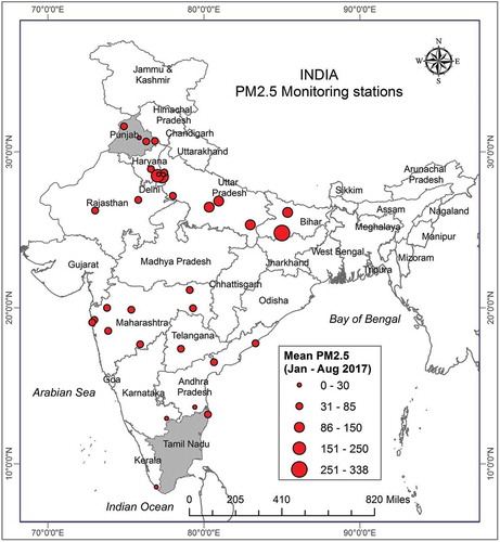
The spatial domain of our study included the Indian subcontinent landmass between 8°44ʹN and 37°06ʹ N latitudes, 68°07ʹ E and 97°25ʹ E longitudes. It includes 3.287 million square kilometers in area and land boundary length of 15,200 km with a coastline of 7,517 km (Figure 1). India is home to the Indo-Gangetic plain (IGP), one of the largest river basins and also to highly air-polluted place in the world. India’s irrigated area at about 0.68Million sq. km (MOA 2018) is the largest in the world and the total forest and tree cover stand at 0.794 Million sq. km (MOEFCC, 2015). India has high regional climatic diversity, concerning location, altitude, distance from sea and relief. The annual rainfall ranges from 300 mm to 650 mm. Temperatures usually range from 25°C to 40°C during summer throughout central India, while the northern Himalayan belt experiences perennial temperatures between 15°C and 20°C (MOES 2015). The country has four seasons, winter (January to March), summer (April to June), monsoon (July to September), post-monsoon (October to December), with winter recording high air pollution levels. During winter, because of the low temperature and shallow boundary layer, there is a presence of a large concentration of aerosol particles near the surface and in the vertical column. Also, there is a strong presence of mineral dust and sea salt during pre-monsoon and monsoon seasons, respectively (Kedia et al. 2014). All these factors, in combination, are major determinants in the quality of air for human survival.

Figure 1. Measured PM_2.5 concentrations (μg/m³) across 33 ground monitoring stations for the study area during January 2017 – August 2017. Tamil Nadu and Punjab states shaded in gray color are chosen for the study on Gap filling where AOD values are missing (Section 4.2 and 5.2).

3. Datasets used

Most pollution concentration information (PM_2.5) is generally obtained from ground monitoring stations that are limited and sparsely located in nature. Further continuous ground pollution monitoring is absent in various regions across the world. In India, the Central Pollution Control Board (CPCB) continuously monitors the ground-level PM_2.5 at 33 locations (Figure 1) under the National Air Quality Monitoring Programme (NAMP) meeting policy standards established according to the National Ambient Air Quality Standards (NAAQS). These site locations are spread across 12 states, with 16 monitors in urban locales and 17 monitors in rural areas. The PM_2.5 concentrations have been estimated under the gravimetric method, where the mass concentrations in ambient air are calculated as the total mass of collected particles in PM_2.5 size ranges divided by the total volume of ambient air sampled, expressed in μg/m³ (CPCB, 2012). The PM_2.5 data were collected from January to August 2017, the study period, totaling to 238 days from 33 stations. This is the first time such data has been collected, and daily average values are published for the entire Indian subcontinent by CPCB.

MODIS (Moderate Resolution Imaging Spectroradiometer) instrument aboard the Terra satellite, part of NASA Earth Observation System (EOS) was launched in May 1999. It has a sun-synchronous, near-polar, circular orbit of 705 km. It has a ground swath of 2330 km with 10 km resolution at the nadir viewing angle. The Terra satellite crosses the equator at 10.30 am (descending node). It has 36 spectral bands, of which bands between 0.412 μm and 2.155 μm are used for retrieving aerosol properties (GSFC, 2012). The Combined Deep Blue Dark Target Aerosol Optical Depth sub-product from the Collection 6 MODIS aerosol products derived during the period between 1 January and 31 August 2017 (Figure 2) are used in this study. The expected error of the product is found to be ±0.05 + 15% (Wei et al. 2019). This sub-product is the combined result of the output of both Deep Blue and Dark Target algorithms to estimate AOD. In Deep Blue algorithm, the 0.412 μm spectral band (known as the blue band) can clearly distinguish between the bright aerosol particles and the dark surface background. The Dark Target retrieval algorithm is used for land surfaces, which are mostly vegetated and not over bright surfaces like desert area. The combined product thus has more retrieval coverage over land surfaces with a 10 km × 10 km spatial resolution (GSFC, 2012) which would be a reasonable resolution to study the country of 3.3 Mill.Sq.km with varied ecosystems from mountains such as Himalayas and the Western Ghats to the deserts of Rajasthan and East coast.

The spatial variables are derived from the Land Use Land Cover map provided by NRSC, ISRO at a spatial scale of 1:250,000 with the spatial resolution of approximately 125 m on the ground. With this spatial resolution, it is possible to compute the extent of open spaces, percentage of forest cover, agricultural areas within 10 km * 10 km cell size, which is the resolution of our primary independent variable, namely, MODIS Aerosol Optical Depth data. In case of the temporal variable, Land Surface Temperature (LST) product from the INSAT 3DR Imager across the Indian subcontinent provided by MOSDAC, ISRO (www.mosdac.gov.in) is used. This is a geolocated pixel product, where every LST pixel is referenced with corresponding longitude and latitude with a spatial resolution of 0.01° × 0.01°. This product also has gaps due to the possibility of failure in retrieving LST for the location. Vector data (shapefile format) of road network of India (www.mapcruzin.com) was used to develop a road density map for 10 x 10 km cell size.

4. Methodology

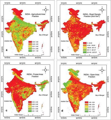
In our earlier study, we had used only AOD values to model the PM_2.5 for the study area using Linear Mixed Effects Model incorporating location as random effect with better accuracy (R²: 0.678 and RMSE: 29.11) compared to LMEM without location as random effect (R²: 0.25, RMSE: 58) (Kesav Unnithan and Gnanappazham 2020). To further improve the accuracy of estimation we used Spatio Temporal Linear Mixed Effect Model (STMEM) where Land Use Land Cover (LULC) information (including percentage cover of open spaces, agricultural area, forest cover and road density), and meteorological data (temperature) were included, which also enable us to quantitatively assess the variation in AOD – PM_2.5 relationship due to each parameter across both space and time. The flow of the modeling process is illustrated in Figure 2. The extent of open spaces, agricultural area, and forest cover are known to impact the concentration of particulate matter at any spatial location (Kloog et al. 2012). Also, the inclusion of road density considers the anthropogenic contribution while temperature models the day-to-day variation in PM_2.5 concentration estimation. Layers of the following four spatial variables are computed for each 10 km × 10 km cell of study area (Figure 3): (i) extent of open spaces, the total area under classes saline marsh, wasteland, and current fallow (ii) extent of forest cover, the deciduous and evergreen forest area present (iii) extent of agricultural area, the total area under cultivation of pre-monsoon, monsoon, post-monsoon seasons and Double/Triple Crop cultivation and (iv) the road density was calculated as the length of major national highways, state highways, and main roads in kilometers that are present in a given 10 km × 10 km grid. The values of resultant spatially varying parameters thus typically range from 0 to 1. Itis assumed in this study that these spatial variables undergo no temporal change during the study period.

Figure 2. Methodology adopted for the estimation of daily PM_2.5 from MODIS AOD over the Indian subcontinent.

Figure 3. Proportionate extent of (a) Agricultural area (b) Road density (c) Forest cover (d) Open spaces calculated within 10 km × 10 km grid.

4.1. Spatiotemporal mixed effects model

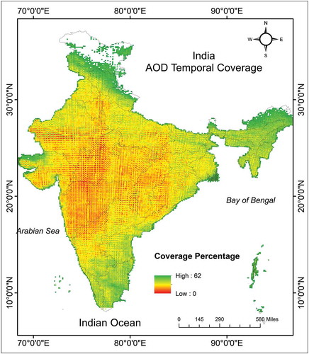
In our earlier study (Kesav Unnithan and Gnanappazham 2020), the calibration was performed by grouping the spatially coincident daily AOD and PM_2.5 values across 33 monitoring stations during the period of January to August 2017. The temporal availability of AOD data which happens to be the major parameter during the study period is illustrated in Figure 4.

Figure 4. Percentage availability of AOD data during the study period of January – August 2017 for the Indian sub-continent.

With the availability of meteorological parameter in the form of daily temperature, the calibration was performed for spatially coincident values of daily AOD, PM_2.5 and temperature and modeled in the following manner.

$\mathrm{P}{\mathrm{M}}_{ij}=\left(\alpha +u_j\right)+\left({\beta }_1+v_j\right)\mathrm{A}\mathrm{O}{\mathrm{D}}_{ij}+\left({\beta }_2+k_j\right)\mathrm{T}\mathrm{e}\mathrm{m}\mathrm{p}\mathrm{e}\mathrm{r}\mathrm{a}\mathrm{t}\mathrm{u}\mathrm{r}{\mathrm{e}}_{ij}+\sum _{m=1}^{m=4}{\gamma }_m^{\hspace{0.17em}}\mathrm{S}{\mathrm{V}}_{im}+s_i+{ϵ}_{ij}$

(1) $\left(u_j{v}_j{k}_j\right)\sim N\left[000,\sum \right]$(1)

where PM_ij represents PM_2.5 concentration at a spatial site i on day j where 1 ≤ i ≤ 33 and 1 ≤ j ≤ 243 for calibration; α, u_j are the fixed and random day-specific intercepts; while β₁, v_j represents fixed and random day-specific slopes for AOD; AOD _ij is the AOD in grid cell corresponding to site i on day j; Temperature _ij is temperature at grid cell corresponding to site i on day j; β₂,κ_j represents fixed and random day-specific slopes for temperature, $\gamma$_m is the co-efficient corresponding to m^th spatial variable where 1 ≤ m ≤ 4 (extent of open spaces, agricultural area, forest cover, and road density); SV_im is the m^th spatial variable of i^th site, whereas s_i is site bias term associated with spatial site i and ϵ_ijis the error term for grid corresponding to site i on day j.

As mentioned above, there exists random slopes and intercepts for both AOD and Temperature variables which are used to map the temporal variability in the AOD – PM_2.5 relationships more accurately. Also, the spatial variability of the relationship is taken care by the location-specific site bias term S_i. Also, the spatial variables are added as random intercept terms since they are assumed to have no temporal variability within the study period. The spatial variables such as road density, agricultural cover, open spaces, and forest area (Figure 3) are included to model the overall spatial variability in the AOD – PM_2.5 relationships. There are 53 metropolitan cities distributed across and 3984 other cities and towns in the country connected by a network of 115,435 km total length of national highways, a continuous source of aerosol which makes the road density a crucial variable to get included in the model. India is an agricultural country with more than 60% of the land is under agriculture cultivated in either two or three seasons a year, while postharvest activities become another important source of aerosol particle. Similarly, there exists ~20% of open land across the country, which also accounts for the overall aerosol particles emitted into the atmosphere. Hence, we included the probability of agricultural cover, forest cover, and open land as other important variables in modeling PM_2.5 concentrations.

It can be observed from Table 1 that the number of co-incident AOD, PM_2.5, and temperature values for the implementation of STMEM is comparatively lesser than the number of observations recorded for spatially coincident AOD and PM_2.5 values of LMEM. The number of days of observation for STMEM where there are more than two sets of values of AOD, PM_2.5 and Temperatures data has also reduced compared to LMEM. There is, however, greater mapping of the spatial variability of the AOD – PM_2.5 relationships as evident from the greater number of coefficients for those spatial variables. The fixed effect coefficients represent the overall relationship between the model variables, whereas the random effect coefficients are derived for each day during the modeling period. This translates as 157 random slope coefficients and 157 intercept coefficients for PM_2.5 and temperature, along with 33 site-bias random intercepts totals to 661 random coefficients for STMEM. Various combinations of temporal and spatial variables, including (i) open spaces and agricultural areas (ii) open spaces and forest cover area (iii) open spaces, agricultural areas, forest cover areas, and temperature (iv) open spaces, agricultural areas, forest cover areas, temperature data, and road density were analyzed to ascertain which among these combinations exert a greater influence on the AOD – PM_2.5 relationships.

Table 1. Statistical summary of parameters associated with the spatiotemporal mixed effects model.

Parameters	STMEM	LMEM
Number of Stations (i)	33	33
Number of Days (j)	157	168
Number of co-incident observations of AOD and PM2.5 (Temperature observations included for STMEM)	599	885
Number of Fixed Effect Coefficients	7	2
Number of Random Effect Coefficients	661	369

4.2. Interpolation integrated spatio-temporal mixed effects model

There was a unique requirement in that there was a necessity for day-wise/month wise PM_2.5 concentrations across all places in India to be estimated that was to be consistent with an overall estimation of the proposed mixed-effects model. Thus, there was a need to propose and develop a novel technique to estimate the PM_2.5 concentrations at spatial locations where AOD retrieved values were not available owing to the onset of monsoon. We attempted to include a mixed-effects model in conjunction with spatial interpolation techniques such as Ordinary Spatial Kriging, Inverse Weighted Distance (IDW) Method and Ordinary Spline Interpolation. A spatial subset of the PM_2.5 concentration layers of STMEM outputs was taken into consideration for this study. The States of Tamil Nadu from south and Punjab from the north were chosen for the application of Spatio-Temporal Interpolation of PM_2.5 concentration using the Mixed Effects Model with spatial kriging, IDW method, and spline interpolation method and the results were compared. This study area was chosen since there existed a good number of cells with both estimated PM_2.5 concentrations and no estimates due to lack of AOD values facilitating interpolation.

Tamil Nadu is the sixth most populous state in the country and eleventh largest by areawith130,060sq.km. The state has a total road length of 167,000 km with a forest cover of 26,345 square kilometers and agricultural area of 43,000 sq.km (www.tn.gov.in). Tamil Nadu has one PM_2.5 monitoring station, Chennai; however, the model could be influenced by nearby three stations at Tirupati, Bangalore, and Thiruvananthapuram. While Punjab lies north west of the country with intensive cropped area under 40, 230 sq.km out of 50, 362 sq.km total area of the state. Forest cover of the state is 2930 sq.km. Punjab has three monitoring stations, namely, Amritsar, Ludhiana, and Mandin Gobingarh and influenced by Panchkula station of Punjab. This model extension was taken into consideration, as shown in the following equation by employing the estimated PM_2.5concentrations by the STMEM as described in the previous section. It estimates the value by combining PM_2.5 of the locations estimated by STMEM and interpolation techniques such as Spatial Kriging, IDW method and Spline interpolation for locations having voids in estimated PM_2.5.

(2) $P{M}_{ij}=\left(\alpha +u_i\right)+\left(\beta +v_i\right)MeanP{M}_j+\gamma \ast Interpolate(X,Y{)}_{ij}+{ϵ}_{ij}$(2)

where PM_ij is the estimated mean PM_2.5 at cell i for month j; α, u_j are the fixed and random month – specific Intercepts; β, v_j are the fixed and random month – specific Slopes for AOD; Mean PM_j is the mean PM2.5 over space for month j; γ represents the fixed weight of the interpolated value; Interpolate (X,Y)_ij is interpolated PM_2.5 concentration value for the month j by the chosen algorithm (IDW, Kriging, and Spline) for ith cell; and ϵ_ij represents the Error term for grid corresponding to site i on month j. The PM_2.5 concentration for spatial locations without AOD input values can be estimated according to the above equation. With higher computing power and storage capacity, the gap-filling for PM_2.5 concentration can be easily scaled up to include daily PM_2.5 concentration layers over a larger study domain.

5. Results and discussion

5.1. Estimated PM_2.5 concentrations by the spatiotemporal mixed effects model

The PM_2.5 concentration was estimated based on both the temporal variation modeled by the temperature value grouped by each day during the study period, and the spatial variation was modeled by including road density ($\gamma$₁), open spaces ($\gamma$₂), agricultural area ($\gamma$₃), and forest cover ($\gamma$₄). The combination of these variables were used in modeling the AOD-PM_2.5 relationship including model M1 – Open spaces and Agricultural area (OA), model M2 – Open spaces and Forest cover (OF), model M3 – Open spaces, Agricultural area, Forest cover area, and Temperature data (OAFT) and model M4 – Open spaces, Agricultural area, Forest cover area, Temperature and Road density data (OAFTR). Each of these models were employed on the same number of daily PM_2.5-AOD pairs (157). Table 2 denotes the values of the model parameters associated with STMEM including all the variables mentioned earlier. The fixed model parameters (α, β_1, β_2,$\gamma$₁, $\gamma$₂, $\gamma$₃, $\gamma$₄) were found to be statistically significant with p-value <0.001, and SE of the order of 0.03. The resulting R² values for the models M1, M2, M3, M4 was 0.569, 0.560, 0.540, and 0.750 with other statistics (Figure 5) shows that M4 could predict close to observation than other models. While comparing with our earlier study on LMEM, improved prediction accuracy was obtained using STMEM with reduced Root Mean Square Error (RMSE) and Mean Bias Error (MBE) of 20.01, 0.11, respectively, when compared with LMEM of our earlier study (RMSE: 29.11 and MBE: 3.22)(Figure 6).

Figure 5. Scatterplot showing the measured and estimated PM_2.5 (μgm/m³) using spatiotemporally modified MEM with the combination of variables (a) M1 – Open spaces and Agricultural area (OA with cross); (b) M2 – Open spaces and Forest cover (OF with minus); (c) M3 – Open spaces, Agricultural area, Forest cover area and Temperature data (OAFT with plus); (d) M4 – Open spaces, Agricultural area, Forest cover area, Temperature and Road density data (OAFTR with dots).

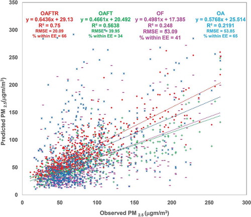
Figure 6. Validation of LMEM and STMEM outputs against observed PM_2.5 levels across 33 stations between January and August 2017.

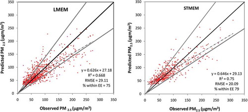
Table 2. Values of fixed effect coefficients of the spatiotemporal mixed effects model including road density $(\gamma$₁₎, open spaces ($\gamma$₂), agricultural area ($\gamma$₃), and forest cover ($\gamma$₄).

Variables		STMEM	LMEM
Fixed Intercept α		3.977	4.417
Fixed Slope (AOD) β1		1.627 * 10^−4	2.050 * 10^−4
Fixed Slope (Temp) β2		−1.830 * 10^−2	-
Fixed coefficients	Road density ($\gamma$1)	1.156	-
	Open space ($\gamma$2)	0.692	-
	Agriculture ($\gamma$3)	0.817	-
	Forest Cover ($\gamma$4)	4.800 * 10^−4	-
Mean Random Intercept (uj)		5.312 * 10^−6	0.169
Mean Random AOD Slope (vj)		6.769 * 10^−5	2.3965 * 10^−4
Mean Site Bias (si)		1.7 * 10^−4	0.391
Mean Random Temperature Slope (kj)		−0.005	-

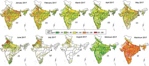
As in the case of estimation of the PM_2.5 byLMEM, a gradual decrease in concentration across the entire study region from an average 142 μg/m³ in January to 103 μg/m³ in April 2017 is observed as depicted in Figure 7. However, the magnitude of the concentration in general has increased across the entire country from a mean PM_2.5concentration of 71μg/m³ from LMEM to 124 μg/m³ obtained from STMEM.

Notably, there is a high loading of PM_2.5 concentrations not only in IGP, but also in the Northwestern parts of the country, including Rajasthan, parts of Madhya Pradesh, and Gujarat. The mean PM_2.5during January 2017 is as high as 142 μg/m³ compared to that of 110 μg/m³ during April 2017. The PM_2.5 concentration estimated using STMEM is comparable to the average PM_2.5 concentrations greater than 100 μg/m³ during the study period reported by PM_2.5 ground monitoring stations across Haryana, Delhi, Uttar Pradesh, and Bihar as shown in an earlier study (Kesav Unnithan and Gnanappazham 2020). Similar PM_2.5 concentrations in the range of 90–110 μg/m³ were reported for the above areas by application of the mixed-effects model (CPCB, 2012). The minimum PM_2.5 concentration map shows that the PM_2.5values in the order of 93 ± 25μg/m³for parts of the country including Maharashtra, Uttar Pradesh, Bihar, Jharkhand, and West Bengal. It can also be seen that like LMEM, even the minimum PM_2.5 concentration estimated by the STMEMis recognized as unhealthy for people suffering from respiratory illness. The maximum value of the PM_2.5 for parts of IGP and central parts of Madhya Pradesh, Odisha, Chhattisgarh, and Telangana is in the order of 170 ± 70 μg/m³, which has been known to have unhealthy to hazardous impact on healthy human according to the Air Quality Index (AQI) (Anderson and Thundiyil 2012), while the maximum PM_2.5 concentrations as estimated by the STMEM stands at 98 ± 15μg/m³ for the entire country.

Figure 7. Estimated PM_2.5 concentrations (μg/m³) during January – August 2017 (a – h), Minimum (i) and Maximum (j) for Indian subcontinent using spatiotemporal mixed effects model including open spaces, forest cover, agricultural areas, road density, and temperature.

A point of interest is that STMEM derives the relationship between daily averaged PM_2.5 values and AOD values derived from MODIS imagery at 10.30 am along with spatial parameters mentioned above. This was because PM_2.5 data for India is available only as daily average value for CPCB stations across the entire country. Also, it was the first time such PM_2.5 concentration is available publicly, which provides a platform to analyze the PM_2.5 concentration values both spatially and temporally. Also, to be noted is the limited number of PM_2.5 sampling stations that provide consistent and gap-free data length for the study period considered. Besides, the AOD values derived from satellite data, PM_2.5 values are affected by physical factors including Planetary Boundary Layer (PBL), windspeed, relative humidity, mixing ratio as well as the atmospheric composition prevalent at a spatial location (Miao et al. 2019). Hence, deriving daily surface PM_2.5 concentrations from AOD is a complex and time-consuming process. Considering all these limitations, we modeled the relationship between satellite-derived AOD and daily surface PM_2.5 concentrations using the 33 stations’ dailyPM_2.5 measurements across the country. STMEM considering different spatio-temporal variables shows that there exists some meaningful relationship in estimating the daily PM_2.5 concentrations spatially from MODIS AOD across the Indian subcontinent despite the limitations mentioned above.

It is visible from the maps of the monthly average of daily estimatedPM_2.5 values from June to August 2017 (Figure 7(f–h)) that there are large gaps in estimated PM_2.5 values throughout central India. This is mostly related to corresponding gaps in AOD retrieval due to the onset of the monsoon climate associated with July to September. This limitation inhibits the model’s capacity to gainfully estimate ground-level PM_2.5 concentrations during periods that needs intensive computations. As was the case with the estimation of PM_2.5 concentration values from LMEM, there are inherent gaps in estimated PM_2.5 concentration by the STMEM throughout central India. Thus, the logical completion of this study would be by estimating PM_2.5 concentrations in spatial sites where no AOD data has been retrieved which was carried out using Interpolation integrated STMEM.

5.2. Gap filling of PM_2.5 concentration using interpolation integrated spatio-temporal mixed effects model

MEM coupled with spatial interpolation methods for each 10 km * 10 km pixel is implemented for Tamil Nadu and Punjab are shown in Figures 8 and 9 for April 2017 and is validated against CPCB monitoring station at Chennai and Mandin Gobingarh, Ludhiana, and Amritsar of Punjab.

STMEM output for April 2017 across the Indian subcontinent is combined with Inverse Distance Weighted, Kriging, and Spline interpolation methods to interpolate the PM_2.5 to fill the gaps in estimation due to AOD unavailability. The mean concentration of PM_2.5for the month of April 2017 for the entire state as obtained using STMEM integrated with IDW, Kriging, and Spline algorithms are 92 ± 58 μg/m³, 90 ± 47μg/m³ and 95 ± 39μg/m³ respectively for Tamil Nadu and 137 ± 168 μg/m³, 135 ± 11 μg/m³ and 142 ± 22 μg/m³ respectively for Punjab. The interpolated STMEM value of monitoring stations are verified with the observed PM_2.5value for Chennai (99μg/m³), Amritsar (34 μg/m³), Ludhiana (46 μg/m³) and Mandin Gobingarh (73 μg/m³).The estimation using IDW, Kriging, and Spline for Chennaiare93.3μg/m³, 92.5μg/m³, 95.2μg/m³ respectively showing the spline method is close to observation. The estimated value using IDW, Kriging, and Spline are 105 μg/m³, 142 μg/m³ and 96 μg/m³for Mandin Gobingarh; are 64 μg/m³, 116 μg/m³ and 51 μg/m³ for Amritsar and 119 μg/m³, 135 μg/m³ and 119 μg/m³ for Ludhiana, respectively. Thus, mean PM_2.5 value obtained from the Mixed Effects Model using Spline technique has shown more correlation with the known mean PM_2.5 concentration for the study area Chennai, followed by Mandin Gobingarh and Amritsar while the variation is higher for Ludhiana by all three methods. Such very high variation by all three methods could be due to the higher variance of the input PM_2.5 values (Figure 9(a)) for the interpolation integrated STMEM model. Hence, based upon the above case study, it can be gainfully said that MEM implementation using ordinary spline interpolation can efficiently estimate PM_2.5 concentrations at spatial locations where no AOD data is available.

Figure 8. (a) PM_2.5 concentrations for April 2017 (b) Gap – filled spatiotemporal interpolation by mixed effects model implemented using spline interpolation (c) using ordinary kriging (d) using the IDW method of Tamil Nadu.

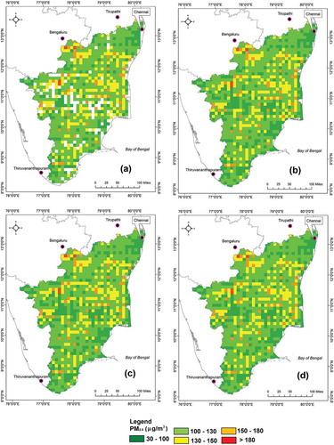
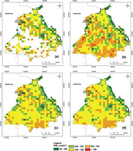
Figure 9. (a) PM_2.5 concentrations for April 2017 (b) Gap – filled spatiotemporal interpolation by mixed effects model implemented using spline interpolation (c) using Ordinary Kriging (d) using the IDW method for Punjab.

6. Conclusion

A network of 33 stations across the country was installed by CPCB to monitor ground-level PM_2.5 concentrations. However, there exist significant gaps in monitoring across the central, as well as the northeastern parts of the country. Estimating PM_2.5 levels in such gaps using satellite data with high spatiotemporal resolution will help in monitoring the pollution levels across the country. An outcome of such satellite data-based models to estimate air quality parameters would be of significant use to management authorities to monitor the trend of air quality, to control and regulate the pollution levels and fixing the air quality standards for industrial and town planning g (Givoni 1991).

This study demonstrated how AOD values obtained through satellite remote sensing data could be useful in estimating ground-level PM_2.5 concentrations with the implementation of STMEM. Our study to model daily PM_2.5 over the Indian sub-continent region using satellite-derived AOD and significantly distributed network of PM_2.5 monitoring stations confirms with the earlier studies conducted in western countries. The model with an expected error of 14%, RMSE of 20.09 with a regression coefficient of 0.75 is more practical in its application since it enables to model day-to-day variations in the AOD – PM_2.5 relationships, which is unique for each day during the study period, mostly influenced by spatial and temporal variables. Our results of STMEM show that temporal variables such as rainfall, humidity, and the point source of pollution including industries, stubble burning, need to be carefully studied and incorporated for the accurate mapping and estimation of air pollution levels. India has varied ecological regimes from very humid to arid including desert and mountain stretch along with coastal stretch. Hence, accurate estimation of ecosystem-specific PM_2.5 would be a challenging which could also be taken up using recently available 3 km AOD data product which with a more reliable estimate on AOD (Remer et al. 2013; Gupta et al. 2018). Further, gap-filling methods carried out with the help of STMEM is a useful indicator for setting up an overall inventory of PM_2.5 across the study region with reasonable accuracy. This study can be taken forward by using spatiotemporal MEM regardless of the unavailability of AOD in few locations in conjunction with GEOS CHEM Model to estimate the buildup of different types of particulate matter.

Highlights

1. Spatio-temporal Mixed Effect Model (STMEM) was able to give a better estimation of PM_2.5 (R2 = 0.75 and RMSE = 20) using MODIS Deep Blue Dark Target AOD product.

2. The daily variation of PM_2.5 was modeled using its relation with satellite-derived AOD values for the first time for the entire country.

3. Inclusion of road density improves the accuracy levels than other parameters such as extent of agriculture, forest, and open space.

4. The study also had shown the Spatial interpolation integrated MEM can be used to fill the gaps in the estimation of PM_2.5 because of the non-availability of AOD for the particular time and location.

Disclosure statement

No potential conflict of interest was reported by the authors.

Additional information

Funding

This work was supported by the Indian Institute of Space Science and Technology, Thiruvananthapuram, India.

References

- Alpert, P., H. Messer, and N. David. 2016. “Mobile Networks Aid Weather Monitoring.” Nature 537 (7622): 617. doi:10.1038/537617e.
- Anderson, J. O., and J. G. Thundiyil. 2012. “Clearing the Air : A Review of the Effects of Particulate Matter Air Pollution on Human Health.” Journal of Medical Toxicology 8 (2): 166–175. doi:10.1007/s13181-011-0203-1.
- Borsdorff, T., J. Aan De Brugh, S. Pandey, O. Hasekamp, I. Aben, S. Houweling, and J. Landgraf. 2019. “Carbon Monoxide Air Pollution on Sub-city Scales and along Arterial Roads Detected by the Tropospheric Monitoring Instrument.” Atmospheric Chemistry and Physics 19 (6): 3579–3588. doi:10.5194/acp-19-3579-2019.
- Bozzo, A., A. Benedetti, J. Flemming, Z. Kipling, and S. Remy. 2019. “An Aerosol Climatology for Global Models Based on the Tropospheric Aerosol Scheme in the Integrated Forecasting System of ECMWF.” Geoscientific Model Development Discussions. doi:10.5194/gmd-2019-149.
- “Central Pollution Control Board, National Ambient Air Quality Series: NAAQMS. 36.” Guidelines for the Measurement of Ambient Air Pollutants. 2012.
- Chacko, S., C. Ravichandran, S. M. Vairavel, and J. Mathew. 2019. “Employing Measurers of Spatial Distribution of Carbon Storage in Periyar Tiger Reserve, Southern Western Ghats, India.” Journal of Geovisualization and Spatial Analysis 3 (1): 1. doi:10.1007/s41651-018-0024-8.
- Chameides, W., H. Yu, S. Liu, M. Bergin, X. Xhou, L. Mearns, and F. Giorgi. 1999. “Study of the Effects of Atmospheric Regional Haze on Agriculture : Enhance Crop Yields in China through Emission Controls?” Proceedings of the National Academy of Sciences 96 (24): 13626–13633. doi:10.1073/pnas.96.24.13626.
- Chowdhury, S., and S. Dey. 2016. “Cause-specific Premature Death from Ambient PM2.5 Exposure in India: Estimate Adjusted for Baseline Mortality.” Environment International 91: 283–290. doi:10.1016/j.envint.2016.03.004.
- Chu, Y., Y. Liu, X. Li, Z. Liu, H. Lu, Y. Lu, and H. Xiang. 2016. “A Review on Predicting Ground PM2.5 Concentration Using Satellite Aerosol Optical Depth.” Atmosphere 7 (10): 1–25. doi:10.3390/atmos7100129.
- Chudnovsky, A. A., A. Kostinski, A. Lyapustin, and P. Koutrakis. 2013. “Spatial Scales of Pollution from Variable Resolution Satellite Imaging.” Environmental Pollution 172 (January): 131–138. doi:10.1016/j.envpol.2012.08.016.
- Curtius, J. 2006. “Nucleation of Atmospheric Aerosol Particles.” Journal of Comptes Rendus Physique 7: 1027–1045. doi:10.1016/j.crhy.2006.10.018.
- Dey, S., L. Di Girolamo, A. van Donkelaar, S. N. Tripathi, T. Gupta, and M. Mohan. 2012. “Variability of Outdoor Fine Particulate (PM 2.5) Concentration in the Indian Subcontinent: A Remote Sensing Approach.” Remote Sensing of Environment 127: 153–161. doi:10.1016/j.rse.2012.08.021.
- Di Nicolantonio, W., and A. Cacciari. 2011. “MODIS Multiannual Observations in Support of Air Quality Monitoring in Northern Italy.” Italian Journal of Remote Sensing 43: 97–109.
- Filonchyk, M., H. Yan, and Z. Zhang. 2019. “Analysis of Spatial and Temporal Variability of Aerosol Optical Depth over China Using MODIS Combined Dark Target and Deep Blue Product.” Theoretical Applied and Climatology 137 (3–4): 2271–2288. doi:10.1007/s00704-018-2737-5.
- Givoni, B. 1991. “Impact of Planted Areas Urban Environmental Quality : A Review.” Atmospheric Environment 25 (3): 289–299.
- Global Burden of Disease Collaborative Network. 2017. “Global Burden of Disease Study 2016 (GBD 2016).” Institute for Health Metrics and Evaluation (IHME).
- Global Burden of Diseases MAPS Working Group. 2018. “Burden of Diseases Attributable to Major Air Pollution Sources in India.” Special Report 21. Health Effects Institute (HEI).
- GSFC (Goddard Space Flight Centre). 2012. “National Aeronautical Space Agency (NASA), Understanding MODIS Products.”
- Gupta, P., L. A. Remer, R. C. Levy, and S. Mattoo. 2018. “Validation of MODIS 3 Km Land Aerosol Optical Depth from NASA’s EOS Terra and Aqua Missions.” Atmospheric Measurement Techniques 11: 3145–3159. doi:10.5194/amt-11-3145-2018.
- Gupta, P., S. A. Christopher, J. Wang, R. Gehrig, Y. Lee, and N. Kumar. 2006. “Satellite Remote Sensing of Particulate Matter and Air Quality Assessment over Global Cities.” Atmospheric Environment 40: 5880–5892. doi:10.1016/j.atmosenv.2006.03.016.
- Habib, A., B. Chen, G. Shi, Y. Iwasaka, D. Nath, B. Khalid, … D. Ntwali. 2019. “Dust Particles in Free Troposphere over Chinese Desert Region Revealed from Balloon Borne Measurements under Calm Weather Conditions.” Atmospheric and Oceanic Science Letters 12 (1): 12–20. doi:10.1080/16742834.2019.1536645.
- Han, Y., Y. Wu, T. Wang, B. Zhuang, S. Li, and K. Zhao. 2015. “Impacts of Elevated-aerosol-layer and Aerosol Type on the Correlation of AOD and Particulate Matter with Ground-based and Satellite Measurements in Nanjing, Southeast China.” Science of the Total Environment 532: 195–207. doi:10.1016/j.scitotenv.2015.05.136.
- Kaufman, Y. J., D. Tanré, and O. Boucher. 2002. “A Satellite View of Aerosols in the Climate System.” Nature 419: 215–223. doi:10.1038/nature01091.
- Kedia, S., S. Ramachandran, B. N. Holben, and S. N. Tripathi. 2014. “Quantification of Aerosol Type, and Sources of Aerosols over the Indo-Gangetic Plain.” Atmospheric Environment 98: 607–619. doi:10.1016/j.atmosenv.2014.09.022.
- Kesav Unnithan, S. L., and L. Gnanappazham. 2020. “Estimation of PM2.5 From MODIS Aerosol Optical Depth over the Indian Subcontinent.” In Applications of Geomatics in Civil Engineering. Lecture Notes in Civil Engineering, edited by J. Ghosh and I. da Silva. Vol. 33. Singapore: Springer. 249–262.
- Khedikar, S., R. Balasubramanian, N. Chattopadhyay, G. Beig, and N. Kulkarni. 2018. “Monitoring and Study the Effect of Weather Parameters on Concentration of Surface Ozone in the Atmosphere for Its Forecasting.” Mausam 69 (2): 243–252.
- Kloog, I., F. Nordio, B. A. Coull, and J. Schwartz. 2012. “Incorporating Local Land Use Regression and Satellite Aerosol Optical Depth in a Hybrid Model of Spatiotemporal PM2.5 Exposures in the Mid-atlantic States.” Environmental Science and Technology 46 (21): 11913–11921. doi:10.1021/es302673e.
- Kloog, I., P. Koutrakis, B. A. Coull, H. J. Lee, and J. Schwartz. 2011. “Assessing Temporally and Spatially Resolved PM2.5 Exposures for Epidemiological Studies Using Satellite Aerosol Optical Depth Measurements.” Atmospheric Environment 45 (35): 6267–6275. doi:10.1016/j.atmosenv.2011.08.066.
- Lee, H. J., Y. Liu, B. A. Coull, J. Schwartz, and P. Koutrakis. 2011. “A Novel Calibration Approach of MODIS AOD Data to Predict PM2.5 Concentrations.” Atmospheric Chemistry and Physics 11 (15): 7991–8002. doi:10.5194/acp-11-7991-2011.
- Lighty, J. S., J. M. Veranth, and A. F. Sarofim. 2000. “Combustion Aerosols : Factors Governing Their Size and Composition and Implications to Human Health Combustion Aerosols: Factors Governing Their Size and Composition and Implications to Human Health.” Journal of Air and Waste Management Association 50: 1565–1618. doi:10.1080/10473289.2000.10464197.
- Liu, C. J., C. Y. Liu, N. T. Mong, and C. C. K. Chou. 2016. “Spatial Correlation of Satellite-derived PM 2.5 With Hospital Admissions for Respiratory Diseases.” Remote Sensing 8 (11): 1–15. doi:10.3390/rs8110914.
- Liu, Y., J. A. Sarnat, V. Kilaru, D. J. Jacob, and P. Koutrakis. 2005. “Estimating Ground-Level PM2.5 In the Eastern United States Using Satellite Remote Sensing.” Environmental Science and Technology 39 (9): 3269–3278. doi:10.1021/es049352m.
- Liu, Y., R. J. Park, D. J. Jacob, Q. Li, V. Kilaru, and J. A. Sarnat. 2004. “Mapping Annual Mean Ground-level PM 2.5 Concentrations Using Multiangle Imaging Spectroradiometer Aerosol Optical Thickness over the Contiguous United States.” Journal of Geophysical Research 109: 1–10. doi:10.1029/2004JD005025.
- Ma, Z., X. Hu, L. Huang, J. Bi, and Y. Liu. 2014. “Estimating Ground-Level PM 2.5 In China Using Satellite Remote Sensing.” Environmental Science and Technology 48: 7436–7444. doi:10.1021/es5009399.
- Miao, Y., J. Li, S. Miao, H. Che, Y. Wang, X. Zhang, R. Zhu, and S. Liu. 2019. “Interaction between Planetary Boundary Layer and PM2.5 Pollution in Megacities in China: A Review.” Current Pollution Report 5: 261–271. doi:10.1007/s40726-019-00124-5.
- MOA. 2018. “Annual Report 2017–2018, Ministry of Agriculture, Govt. Of India.”
- MOEFCC (Ministry of Environment, Forest and Climate Change). 2015. Govt. of India, India State of forest Report (ISFR).
- MOES. 2015. “Ministry of Earth Sciences 2015 Climatology of the Indian Subcontinent.” Govt of India.
- Nichol, J. E., M. S. Wong, and J. Wang. 2010. “A 3D Aerosol and Visibility Information System for Urban Areas Using Remote Sensing and GIS.” Atmospheric Environment 44 (21–22): 2501–2506. doi:10.1016/j.atmosenv.2010.04.036.
- Palve, S. N., P. D. Nemade, and S. D. Ghude. 2016. “The Application of Remote Sensing Techniques for Air Pollution Analysis and Climate Change on Indian Subcontinent.” IOP Conference Series: Earth and Environmental Science 37 (1): 012076. doi:10.1088/1755-1315/37/1/012076.
- Remer, L. A., S. Mattoo, R. C. Levy, and L. A. Munchak. 2013. “MODIS 3 Km Aerosol Product: Algorithm and Global Perspective.” Atmospheric Measurement and Techniques 6: 1829–1844. doi:10.5194/amt-6-1829-2013.
- The Hindu. 2017. “Delhi’s Pollution Levels Rise Again.” http://www.thehindu.com/news/cities/Delhi/after-dip-pollution-levels-riseagain/article20355358.ece
- van Donkelaar, A., and R. V. Martin. 2013. “Optimal Estimation for Global Ground-level Fine Particulate Matter Concentrations.” Journal of Geophysical Research 118: 5621–5636.
- van Donkelaar, A., R. V. Martin, and R. J. Park. 2006. “Estimating Ground-level PM2.5 Using Aerosol Optical Depth Determined from Satellite Remote Sensing.” Journal of Geophysical Research Atmospheres 111 (21): 1–10. doi:10.1029/2005JD006996.
- Wang, B., and Z. Chen. 2016. “High-resolution Satellite-based Analysis of Ground-level PM2.5 For the City of Montreal.” Science of the Total Environment 541: 1059–1069. doi:10.1016/j.scitotenv.2015.10.024.
- Wei, J., Z. Lib, L. Sun, Y. Peng, and L. Wang. 2019. “Improved Merge Schemes for MODIS Collection 6.1 Dark Target and Deep Blue Combined Aerosol Products.” Atmospheric Environment 202: 315–327. doi:10.1016/j.atmosenv.2019.01.016.
- Xie, Y., Y. Wang, K. Zhang, W. Dong, B. Lv, and Y. Bai. 2015. “Daily Estimation of Ground-Level PM 2.5 Concentrations over Beijing Using 3 Km Resolution MODIS AOD.” Environmental Science and Technology 49 (20): 12280–12288. doi:10.1021/acs.est.5b01413.
- You, W., Z. Zang, X. Pan, L. Zhang, and D. Chen. 2015. “Estimating PM2.5 In Xi’an, China Using Aerosol Optical Depth : A Comparison between the MODIS and MISR Retrieval Models.” Science of the Total Environment 505: 1156–1165. doi:10.1016/j.scitotenv.2014.11.024.