Comparative performance of convolutional neural network, weighted and conventional support vector machine and random forest for classifying tree species using hyperspectral and photogrammetric data

ABSTRACT

The classification of tree species can significantly benefit from high spatial and spectral information acquired by unmanned aerial vehicles (UAVs) associated with advanced classification methods. This study investigated the following topics concerning the classification of 16 tree species in two subtropical forest fragments of Southern Brazil: i) the potential integration of UAV-borne hyperspectral images with 3D information derived from their photogrammetric point cloud (PPC); ii) the performance of two machine learning methods (support vector machine – SVM and random forest – RF) when employing different datasets at a pixel and individual tree crown (ITC) levels; iii) the potential of two methods for dealing with the imbalanced sample set problem: a new weighted SVM (wSVM) approach, which attributes different weights to each sample and class, and a deep learning classifier (convolutional neural network – CNN), associated with a previous step to balance the sample set; and finally, iv) the potential of this last classifier for tree species classification as compared to the above mentioned machine learning methods. Results showed that the inclusion of the PPC features to the hyperspectral data provided a great accuracy increase in tree species classification results when conventional machine learning methods were applied, between 13 and 17% depending on the classifier and the study area characteristics. When using the PPC features and the canopy height model (CHM), associated with the majority vote (MV) rule, the SVM, wSVM and RF classifiers reached accuracies similar to the CNN, which outperformed these classifiers for both areas when considering the pixel-based classifications (overall accuracy of 84.4% in Area 1, and 74.95% in Area 2). The CNN was between 22% and 26% more accurate than the SVM and RF when only the hyperspectral bands were employed. The wSVM provided a slight increase in accuracy not only for some lesser represented classes, but also some major classes in Area 2. While conventional machine learning methods are faster, they demonstrated to be less stable to changes in datasets, depending on prior segmentation and hand-engineered features to reach similar accuracies to those attained by the CNN. To date, CNNs have been barely explored for the classification of tree species, and CNN-based classifications in the literature have not dealt with hyperspectral data specifically focusing on tropical environments. This paper thus presents innovative strategies for classifying tree species in subtropical forest areas at a refined legend level, integrating UAV-borne 2D hyperspectral and 3D photogrammetric data and relying on both deep and conventional machine learning approaches.

KEYWORDS:

• Tropical diversity
• individual tree crown
• deep learning
• imbalanced sample set
• unmanned aerial vehicle

Introduction

Among Brazilian biomes, the Atlantic Rain Forest, locally known as Mata Atlântica, is a global priority for biodiversity conservation due to its abundance in flora and fauna species (Myers et al. 2000; Laurance 2009; Colombo and Joly 2010). Due to anthropogenic disturbances, such as industrial activities, urbanization, and agricultural expansion, its current vegetation cover was estimated at 16% in 2009 (Ribeiro et al. 2009) and 28% in 2018 (Rezende et al. 2018). The Mixed Ombrophylous Forest (MOF), a phytophysiognomy of the Atlantic Rain Forest and one of the main formations in the southern region of Brazil, is considered one of the most threatened phytophysiognomies and has lost 75.6% of its original coverage (Vibrans et al. 2013). It is characterized by a heterogeneous formation of vegetation with primitive genera, such as Drimys, Araucaria (Australasian) and Podocarpus (Afro-Asian) (Higuchi et al. 2013). Even though legally protected and its harvesting for timber prohibited by law in Brazil, the Araucaria angustifolia species is critically endangered according to the “List of Threatened Species” of the International Union for Conservation of Nature (IUCN 2017).

Currently, one of the main challenges for conservation is to obtain sound and trustworthy information at a large scale to monitor biodiversity, resources, ecosystem services and the anthropogenic impact on natural environments (Wagner et al. 2019). Remote sensing is considered an effective means for this effort, not only because of the increased spatial and temporal resolutions of the datasets, which enable identifying elements of biodiversity, such as tree species, but also because of the increase in available data and in the associated computational capacity to process such data (Ghosh et al. 2014; He et al. 2015; Kwok 2018).

Small-format hyperspectral cameras on-board unmanned aerial vehicles (UAVs) provide high spectral and very high spatial resolution data, substantially increasing the scope of remote sensing applications. UAV-borne sensors enable to collect data even under cloud cover conditions. Moreover, they are flexible regarding spatial and temporal resolution, what makes them a cost-effective and operational solution for many applications (Honkavaara et al. 2013), such as tree species classification (Nevalainen et al. 2017; Tuominen et al. 2018; Sothe et al. 2019a).

Besides the high spatial and spectral resolution data, UAV-borne sensors operating in frame format record spectral data in two spatial dimensions at each exposure, allowing for the extraction of 3D information via imaging spectroscopy (Aasen et al. 2018). This information can capture differences in vertical structure among tree species (i.e. tree height, tree patterns and leaf distributions) (Näsi et al. 2015; Tuominen et al. 2018) that can be valuable for tree species classification. Over the last years, many studies have shown some improvement in accuracy when integrating multispectral or hyperspectral data with 3D information (e.g., derived from Light Detection and Ranging-LiDAR data or PPC) for tree species classification (Dalponte, Bruzzone, and Gianelle 2012; Ghosh et al. 2014; Baldeck et al. 2015; Piiroinen et al. 2017; Tuominen et al. 2018; Sothe et al. 2019a). This combination allows to obtain a richer description of the analyzed vegetation, as these sources of information are complementary to each other (Ghosh et al. 2014), but until now they have been poorly explored in tropical forests.

The classification of tree species with high spatial resolution hyperspectral images is performed mainly at an individual tree crown (ITC) or at a pixel scale (Shen and Cao 2017). At a pixel scale, species identification is conducted using classification approaches based on the spectral information of each pixel. However, the presence of noise, differences in lighting conditions and spectral variability within the crowns, such as branches, presence of lianas, background, shadow, may negatively affect the classification results. At an ITC scale, object-based approaches use tree crowns as classification units, reducing the effects of spectral variability of pixels (Heinzel and Koch 2012). In this sense, many studies showed that the classification of tree species at an ITC level using object-based image analysis (OBIA) or the majority vote rule (MV) approaches has proved to be more accurate than that executed at a pixel scale (Clark, Roberts, and Clark 2005; Clark and Roberts 2012; Dalponte et al. 2013; Féret and Asner 2013). Furthermore, a classification map at an ITC level may be more easily related to the biophysical and biochemical properties of the species and has practical applications in studies of individual trees (Dalponte et al. 2014; Shen and Cao 2017).

Besides the data and the classification approach, the classification method is also decisive for a precise land use and cover mapping (Lu and Weng 2007). In this respect, machine learning algorithms, such as support vector machine (SVM) and random forest (RF), have been on the spotlight for tree species classification over the last years (Dalponte, Bruzzone, and Gianelle 2012; Ghosh et al. 2014; Baldeck et al. 2015; Ballanti et al. 2016; Ferreira et al. 2016; Piiroinen et al. 2017; Franklin and Ahmed 2017; Maschler, Atzberger, and Immitzer 2018; Ferreira et al. 2019). These methods are considered robust and work well in the presence of a wide range of class distributions (Andrade, Francisco, and Almeida 2014) and with high dimensionality and multisource data (Ghosh et al. 2014).

Nevertheless, even with the availability of high spectral and spatial resolution data and robust classifiers, it is observed that studies involving tropical forests have been limited to the classification of three to eight dominant canopy species (e.g., Clark, Roberts, and Clark 2005; Clark and Roberts 2012; Baldeck et al. 2015; Ferreira et al. 2016; Shen and Cao 2017). Among the issues that hamper the classification of a high number of tree species in such environments, the presence of dominant and minority classes is to be mentioned, resulting in an imbalanced sample set, with a small number of samples available for the less often found tree species (Mellor et al. 2015). In this case, sampling the natural abundance of species would lead to highly skewed sample sizes across classes, while increasing the sample sizes of rare species would be time-consuming and costly (Graves et al. 2016). Concerning this, some approaches relying on machine learning have been adapted to deal with small or imbalanced sample sets (Dalponte et al. 2015; Graves et al. 2016; Nguyen, Demir, and Dalponte 2019). Dalponte et al. (2015) proposed a semi-supervised SVM to combine the information from both labeled and unlabeled sets as a way to increase the number of samples. Graves et al. (2016) investigated the imbalanced classes problem with two strategies: i) creating a dataset where every class has the same amount of training samples, equal to the number of samples of the smallest class; and ii) allowing different cost parameters for each class while using the SVM classifier. Nguyen, Demir, and Dalponte (2019) proposed a weighted SVM (wSVM) method specifically developed to solve the problems of unbalancing, unreliability, and size of the training sets for tree species classification at an ITC level.

Although conventional machine learning methods such as RF and SVM are very well established in literature, these methods are based on hand-engineered features, and are thus highly dependent on domain knowledge (Li, Zhang, and Shen 2017). Recently, deep learning has been introduced into hyperspectral images classification and is able to extract deep spatial and spectral features from hyperspectral data (Signoroni et al. 2019). Much of the pioneering work on deep learning applied to hyperspectral data classification has given evidence that the identification of deep features leads to higher classification accuracies for hyperspectral data (Chen et al. 2014; Li et al. 2017; Wagner et al. 2019). Among these methods, the convolutional neural network (CNN) algorithm is a supervised deep learning model that has produced promising results in the classification of remotely sensed images (Yue et al. 2015; Li, Zhang, and Shen 2017; Wang et al. 2017; Gao, Lim, and Jia 2018), including tree species classification purposes in particular (Pölönen et al. 2018; Fricker et al. 2019; Hartling et al. 2019). Despite its great potential, to the best of our knowledge, there are no studies involving CNN for tree species classification in tropical or subtropical forests.

Considering what was above exposed, two MOF fragments belonging to the Atlantic Rain Forest biome were analyzed in this study. These areas comprise many tree species with both coniferous and broadleaves mixed together, frequently resulting in imbalanced sample sets. Therefore, this study was committed to evaluate the pure and combined use of high spectral and spatial resolution data acquired by a UAV and their PPC, associated with machine and deep learning methods for the classification of a large number of tree species (refined legend level). Concerning the imbalanced sample sets, this paper investigated a new weighted SVM classifier specifically developed to solve the problems of unbalancing, unreliability, and size of the training sets for tree species classification (Nguyen, Demir, and Dalponte 2019), and a CNN architecture associated with a previous step to balance the number of samples per class. The following hypotheses were tested: i) the inclusion of 3D features derived from the PPC to the 2D hyperspectral data improves the tree species classification; ii) the use of ITC as a classification unit (i.e. object-based approach or by means of the MV rule at an object level) increases the tree species classification accuracies of machine learning methods in relation to the pixel-based classification; iii) classifiers dealing with the imbalanced samples can increase the accuracy of less represented classes; iv) the CNN algorithm can effectively classify tree species using fewer features than conventional machine learning methods with comparable accuracy indices. Hereafter we use the term machine learning to refer to conventional machine learning approaches that do not rely on deep learning.

Material

Study areas

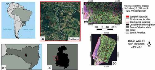
The study areas are located in the southern region of Brazil, in the municipality of Curitibanos, Santa Catarina state (Figure 1). The areas cover an extension of approximately 30 ha (Area 1) and 19 ha (Area 2). They belong to the Atlantic Rain Forest biome and the MOF phytophysiognomy. According to the Köppen–Geiger classification, the climate is Cfb, moist mesothermal with no clearly defined dry season, with a mean annual temperature of 15°C and a yearly rainfall of 1,616 mm (Peel, Finlayson, and Mcmahon 2007). The MOF formation of the study areas is classified as Montane, located approximately at 750 m above sea level (IBGE, 2012).

Figure 1. Study areas and samples location. (a) Santa Catarina state; (b) Curitibanos municipality; (c) Zoom showing the areas location (Google Earth); (d) Area 1; (e) Area 2.

Input data

The hyperspectral data were acquired in a flight executed in December 2017 (spring season), using a quadcopter UAV (UX4 model) and a frame format hyperspectral camera (Senop Ltd. 2018) based on a Fabry–Perot interferometer (FPI), model 2015 (DT-0011). The camera contains one irradiance sensor and one global navigation satellite system (GNSS) receiver.

The hyperspectral imager FPI technology operates on the time-sequential principle (Honkavaara et al. 2017). The camera has two CMOSIS CMV400 sensors that by means of an adjustable air gap are flexible in selecting up to 25 spectral bands ranging from 500 to 900 nm with the minimum bandwidth of 10 nm at the full width at half maximum (FWHM) (Miyoshi et al. 2018). However, by increasing the number of acquired bands, the acquisition time also increases, resulting in spatial offsets among them that need to be corrected in the processing phase (c.f. Section “Data preprocessing”) (Honkavaara et al. 2013, 2017; Aasen et al. 2018). The final settings concerning the hyperspectral camera consider 25 bands ranging from 506 to 819 nm and FWHM between 12.84 and 21.89 nm.

The aerial surveys were carried out in two consecutive days between 12:55 and 13:16 (UTC-3) in Area 1, and between 10:59 and 11:06 (UTC-3) in Area 2. The flights were conducted keeping a great overlap between the stripes, which enabled the creation of high spatial resolution photogrammetric point clouds (PPCs). On both occasions the illumination conditions were stable, and the weather was sunny. Table 1 shows the characteristics of the camera, of the flight and of the data acquired in the study areas.

Table 1. Characteristics of the camera, flight and data acquired in the study areas.

Characteristic	Description
Focal length	8.6 mm
Field of view	37°
Spatial resolution	11 cm (Area 1) 12 cm (Area 2)
Image dimensions	1,023 × 648 pixels
Flight height/speed	150 m/4m.s
Number of strips	8 (Area 1) 6 (Area 2)
Forward and side overlap	70 and 60% (Area 1) 60 and 50% (Area 2)
PPC density	35 points.m^−2 (Area 1) 25 points.m^−2 (Area 2)

Field data and samples collection

Two fieldworks were carried out over both areas. In the first one, a survey was conducted regarding the tree species diversity and structure and the successional stages of the forest fragments. For this, six rectangular plots with 400 m² were delimited in Area 1 and four in Area 2. Inside each plot, all the trees with DBH (diameter at breast height) greater than 5 cm were measured and identified.

The second fieldwork was carried out in October 2018, after the acquisition of the UAV data. Different from what is observed for land-use/land-cover assessment in field inspections, the species identification of an individual tree must be checked and determined by a trained botanist in situ (Graves et al. 2016). Therefore, it was not possible to adopt a randomization scheme for collecting field samples, and only the tree species which had clearly visible crowns in the images were inspected and identified in the field. Trees with ambiguous appearance were discarded.

Only ITCs visited and identified in the fieldwork were used as samples for the tree species classification. Eighty ITCs representing 14 tree species and identified in Area 1, and 41 ITCs representing 11 tree species in Area 2 were selected (Table 2). Based on the first fieldwork, it was estimated that these species represent nearly 55% and 48% of all the trees species (including suppressed and co-dominant trees) of Areas 1 and 2, respectively. Considering only the dominant trees, they represent approximately 80% of the tree species in both areas. The Ocotea sp. class consists of both Ocotea puberula and Ocotea pulchella species, inasmuch as the former one presents a low number of samples. Before the classification, the ITCs were randomly split in training and test sets, and the latter one was used only for accuracy assessment (c.f. Section “Accuracy assessment and species maps”).

Table 2. Tree species and their respective successional groups and number of ITCs and pixels for each tree species used in the classification process according to the study area (A1 = Area 1 and A2 = Area 2).

				ITCs		Pixel samples
ID	Species	Family	Successional group	A1	A2	A1	A2
a	Luehea divaricata	Malvaceae	initial or late secondary, climatic	5	4	23,624	15,259
b	Araucaria angustifolia	Araucariacea	pioneer or secondary	8	6	27,191	32,925
c	Mimosa scabrella	Fabaceae	pioneer	7	-	25,449	-
d	Lithraea brasiliensis	Anacardiaceae	pioneer, initial secondary or climatic	5	8	17,458	13,553
e	Campomanesia xanthocarpa	Myrtaceae	initial or late secondary	5	3	18,837	7,565
f	Cedrela fissilis	Meliaceae	initial or late secondary, climatic	5	2	24,368	12,910
g	Cinnamodendron dinisii	Canellaceae	late secondary	5	-	6,927	-
h	Cupania vernalis	Sapindaceae	initial or late secondary	5	-	12,475	-
i	Matayba elaeagnoides	Sapindaceae	late secondary	8	-	48,231	-
j	Nectandra megapotamica	Lauraceae	initial or late secondary	8	4	11,247	4,862
k	Ocotea sp.	Lauraceae	initial secondary	9	3	101,884	12,991
l	Podocarpus lambertii	Podocarpaceae	late secondary or climatic	6	4	12,387	21,391
m	Schinus terebethifolius (sp1)	Anacardiaceae	pioneer, initial or late secondary	2	2	4,491	2,646
n	Schinus lentiscifolius (sp2)	Anacardiaceae	initial or late secondary	2	-	6,083	-
o	Erythrina falcata	Fabaceae	initial secondary or climatic	-	2	-	3,663
p	Sebastiania commersoniana	Euphorbiaceae	initial secondary	-	3	-	3,396

Methods

Data preprocessing

Initially, the images digital numbers (DN) were transformed into radiance values with units of photon pixel⁻¹ s⁻¹. After that, black images collected prior to the data captured with covered lens were used for the dark signal correction.

In the geometric processing stage, it was necessary to reconstruct the camera geometry and the orientation of each band. The interior orientation parameters (IOPs) and the exterior orientation parameters (EOPs) were estimated using the so-called on-the-job calibration, after a refinement of the initial values. Such initial values for the camera positions were assessed by the GNSS receiver and involved latitude, longitude, and altitude (flight height plus the average terrain elevation) data (Sothe et al. 2019a). In the sequence, the coordinates of six ground control points (GCPs) for Area 1 and 3 GCPs for Area 2 were added to the project and measured in the corresponding reference images. These points were previously located and surveyed in the field (signalized with lime mortar) on the same day of the flight and had their coordinates acquired by a GNSS RTK Leica GS15. After the bundle adjustment, the final errors of Area 1 in the GCPs (reprojection errors) were 0.03 pixels in the image and 0.003 m in the GCPs. In Area 2, the errors were 0.08 pixels in the image and 0.004 m in the GCPs.

Next, the orthorectification was performed starting with the generation of a dense point cloud. The Digital Surface Models (DSMs) with a ground sample distance (GSD) of 11 cm for Area 1 and 12 cm for Area 2 were generated using the dense matching method. At the last stage, the orthomosaics of all the bands were generated from the orthoimages of each hypercube band. This entire procedure was replicated for each of the 25 spectral bands of each area in order to coregister them regarding the slight positioning difference among bands of the same image caused by the time sequential operating principle of the camera (Honkavaara et al. 2013; Miyoshi et al. 2018). After that, the final discrepancies among the orthorectified image bands were measured using the GCPs and four independent points chosen in the images for Area 1, and the GCPs plus two independent points for Area 2. It was verified an error in x and y of about 0.03 ± 0.06 m among the bands of Area 1, and about 0.07 ± 0.08 m in Area 2, which was judged acceptable for the classification purpose.

The orthomosaics of all the bands were stacked to compose the VNIR dataset. The PPC of the bands centered at the 565 nm wavelength and their DSM were exported to be used for the generation of the PPC features and of the canopy height model (CHM).

Datasets composition

This step consisted in the extraction and selection of features from the hyperspectral data to be used in the classification process. The six sets of features described in Table 3 were explored.

Table 3. Description of features used in this study.

Group	Feature name	Description	Equation	Reference
Spectral bands	VNIR	Wavelengths (ρ) 506 to 819 nm
MNF	MNF	Minimum noise fraction		Green et al. (1988)
VIs	NDVI	Normalized Difference Vegetation Index	NDVI = $\frac{{\rho }_{750}-{\rho }_{650}}{{\rho }_{750}+{\rho }_{650}}$	Rouse et al. (1973)
	PRI	Photochemical reflectance index	PRI = $\frac{{\rho }_{535}-{\rho }_{565}}{{\rho }_{535}+{\rho }_{565}}$	Gamon, Peñuelas, and Field (1992)
	PSRI	Plant senescence reflectance index	PSRI = $\frac{{\rho }_{679}-{\rho }_{506}}{{\rho }_{750}}$	Merzlyak et al. (1999)
	PSSR	Pigment specific simple ratio	PSSR = $\frac{{\rho }_{819}}{{\rho }_{679}}$	Blackburn (1998)
GLCM	SM	Angular second moment	SM = ${\sum }_{i,j=0}^{N-1}\left\{p{\left(i,j\right)}^2\right\}$	Haralick, Shanmugam, and Dinstein (1973)
	con	Contrast	Con = ${\sum }_{i,j-0}^{N-1}pi,j{\left(i-j\right)}^2$
	var	Variance	Var =${\sum }_{i,j=0}^{N-1}{\left(i-\mu \right)}^{2}p\left(i,j\right)$
	hom	Homogeneity	Hom = ${\sum }_{i,j=0}^N\frac{pi,j}{1+{\left(1-j\right)}^2}$
	cor	Correlation	Cor =${\sum }_{i,j=0}^{N}pi.j\frac{\left[\left(i-\mu i\right)\left(j-\mu j\right)\right]}{\sqrt{\left({\sigma }^{2}i\right)\left({\sigma }^{2}j\right)}}$
	ent	Entropy	Ent =
	dis	Dissimilarity	Dis = ${\sum }_{i,j-0}^{N-1}pi,j\left|1-j\right|$
	mean	Textural mean	Mean = $\frac{{\sum }_{i=1}^{N}pxi}{N}$
CHM	CHM	Canopy height model	CHM = $DSM-DTMLiDAR$
PPC	zmax	maximum height of all the points within each pixel
	zmean	mean of all the height points within each pixel
	zq90	90th percentile of height distribution within each pixel
	zq70	70th percentile of height distribution within each pixel
	zq5	5th percentile of height distribution within each pixel
	zentropy	entropy of height distribution within each pixel

Three sets of features were extracted from the hyperspectral bands: the minimum noise fraction (MNF), texture features extracted from the gray-level co-occurrence matrix (GLCM) and vegetation indices (VIs). Based on the eigenvalue stats of the output uncorrelated bands, the first eight MNF components were selected. The texture features were calculated based on three bands corresponding to the green, red and NIR regions of the hyperspectral data (respectively centered at the 565, 679, and 780 nm wavelengths) using the GLCM with a window size of 5 × 5. Besides the NDVI, hyperspectral sensors make it possible to compute other indices at specific wavelengths, such as the photochemical reflectance index (PRI), the plant senescence reflectance index (PSRI), and the pigment specific simple ratio (PSSR), calculated according to Table 3.

The last set of features comprised the CHM and six elevation metrics extracted from the UAV-PPC. The CHM was obtained subtracting the DSM (generated with the PPC data) from the Digital Terrain Model (DTM), this last one created using the LAStools software (Isenburg 2018) based on airborne LiDAR data acquired by a company using the Optech Model 3033 laser scanning sensor, with a density of 1 point.m⁻². The PPC features were computed using an area-based approach with 0.5 m of spatial resolution in the lidR package (Roussel et al. 2018) based on R programming (R Development Core Team 2018).

In order to check the importance of each feature in the classification, we adopted the JM distance, since it is widely used in studies concerning tree species classifications (Dalponte, Bruzzone, and Gianelle 2012; Dalponte et al. 2013, 2015; Ferreira et al. 2019; Sothe et al. 2019a). The JM distance varies between 0 and √2, with higher values indicating higher separability of the class pairs in the bands under consideration (Richards and Jia 2006).

Besides the feature importance, the JM distance was also used as a separability criterion of a search strategy for the feature selection process. In this situation, a wrapper method, the sequential forward floating selection (SFFS) algorithm (Pudil, Novovicová, and Kittler 1994) was adopted for being considered a fast suboptimal search strategy (Dalponte et al. 2013). It is characterized by the presence of both forward and backward selection steps at each iteration. This “floating” behavior allows one to reconsider the selected features at each step, reducing the possibility to stop in a local maximum of the separability measure (Dalponte, Bruzzone, and Gianelle 2012; Dalponte et al. 2013). When associated with a search strategy, the JM distance tends to saturate when the optimal number of features is reached. After extracting the features, different datasets were composed to perform the tree species classifications (Table 4).

Table 4. Description of the datasets according to the features used in the classification process.

Dataset Name	VNIR	CHM	PPC	MNF	GLCM	VI	Total features
VNIR	25	-	-	-	-	-	25
VNIR_CHM	25	1	-	-	-	-	26
VNIR_PPC^a	25	-	6	-	-	-	31
VNIR_PPC_CHM	25	1	6	-	-	-	32
VNIR_PPC_CHM_MNF^a	25	1	6	8	-	-	40
VNIR_PPC_CHM_GLCM^a	25	1	6	-	24	-	56
VNIR_PPC_CHM_VI^a	25	1	6	-	-	4	36
VNIR_PPC_CHM_MNF_VI^a	25	1	6	8	-	4	44
VNIR_MNF_GLCM_VI^a	25	-	-	8	24	4	61
MNF_PPC_CHM^a	-	1	6	8	-	-	15
MNF_PPC_CHM_VI^a	-	1	6	8	-	4	19
FSJM-A1^a	18	1	6	7	10	4	46
FSJM-A2^a	21	1	6	4	14	3	49
full^a	25	1	6	8	24	4	68

^aDatasets not tested in the wSVM and CNN algorithms.

Tree species classification

Three machine learning and one deep learning method were tested: SVM, wSVM, RF and CNN. For the wSVM and CNN algorithms, only the pixel-based classification was conducted, while for the SVM and RF, three approaches were compared: a) a pixel-based classification, b) a pixel-based classification associated with the application of the MV rule at an object level, and c) an object-based classification, termed object-based image analysis (OBIA). Brief descriptions of each method followed by details on the experiments and adopted parameters are given below.

SVM and wSVM

The SVM classifier (Vapnik 1995) is a supervised, non-parametric statistical learning technique, which aims at finding an optimal hyperplane for solving the class separation problem. The optimal hyperplane is the one that maximizes the distance between closest training samples and the separating hyperplane (Melgani and Bruzzone 2004). Since the feature space is partitioned among the classes by a hyperplane, low accuracies are obtained for solving non-linear class boundary problems. Hence, SVMs uses the “kernel-trick” to map the data into a higher dimensional feature space (Fassnacht et al. 2014), allowing for non-linear class boundaries.

The standard SVM algorithm may perform poorly if the set of training samples is highly unbalanced among the classes or contains wrongly labeled samples. This effect stems from the fact that the cost function that guides the training of a standard SVM is equally penalized by misclassified samples. Nguyen, Demir, and Dalponte (2019) proposed the wSVM algorithm to mitigate this problem, giving different weights to different samples and to different classes based on three strategies, two of them explored here: i) using the class abundances to differently weight the samples of the different classes and; ii) using the training samples and their distribution in the feature space to differently weight each training sample.

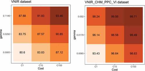
For both SVM and wSVM, the one-against-one multiclass strategy and the radial basis function (RBF) were adopted. This function has two user-defined parameters: cost (C) and gamma (γ). A high value of C may overfit the model to data, while the γ parameter impacts the shape of the separating hyperplane (Li and Du 2015). A 5-fold cross validation was carried out on the training samples set to tune the C parameter, while the γ value was set during the classification process with the function sigest of the kernlab package (Karatzoglou et al. 2004). The value of 100 for parameter C was found to be suitable for all datasets (e.g., Figure 2) and the γ value, defined by sigest, varied between 0.0058 and 0.0283 according to the dataset and study area.

Figure 2. Average accuracy of the 5-fold cross validation procedure to find the best SVM parameters for each dataset. Note: This figure shows the best (right) and worst (left) dataset result for Area 1.

The same process was adopted for the wSVM classification; however, in this case, different weights were applied to each class and each training sample. The algorithms for the computation of the class and sample weights were implemented in R programming based on the k-means clustering (Nguyen, Demir, and Dalponte 2019).

RF

The RF is an algorithm designed by Breiman (2001) aiming to improve the accuracy of classification or regression by combining a large number of trees trained upon random subsets of the available labeled samples and features. In the first case, each tree contributes only one class vote to each instance, and the final classification is determined by the majority votes of all the forest trees (Hastie, Tibshirani, and Friedman 2009). In its simplest form, this algorithm requires the definition of a few parameters: the number of trees to form the “forest” (ntree) and the number of features/predictors considered for each node in the trees (mtry). The method provides a way to evaluate statistical quality by means of an internal sampling procedure called OOB (out-of-bag), which can be used to estimate classification errors and the importance of each feature in the classification process.

Based on a 5-fold cross validation, the RF classifier was preliminarily tested with 100, 500 and 1,000 trees. As also observed by Rodriguez-Galiano et al. (2012), it was found that increasing the number of trees from 100 to 500 led to a small improvement in the classification result, while changing from 500 to 1,000 trees increased the processing time with no corresponding increase in accuracy. In face of this, we opted for using 500 trees in all experiments. It was kept the default value for mtry parameter, which corresponds to the square root of the total number of features used in each experiment (Breiman et al. 2001). The classification was conducted using the randomForest package (Liaw and Wiener 2002) in R programming.

CNN

The first deep learning technique called CNN was introduced by Fukushima (1980), inspired by the animal visual cortex operation, in which each neuron/kernel is focused on processing information associated with a restricted location of the visual field, known as the “receptive field.” The entire visual field is covered by an arrangement of receptive fields of different neurons that partially overlap. CNNs are composed by neurons with learnable weights and biases. Each neuron receives several inputs, extracts a weighted sum over them, passes it through an activation function and responds with an output (Hartling et al. 2019). The four key components of CNN are: a) convolutional layer; b) activation function or non-linearity; c) pooling layer and; d) fully-connected layer (Zhang, Zhang, and Du 2016).

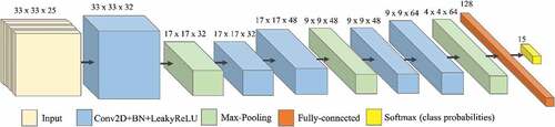
In this study, a CNN architecture was adopted and executed in a Python environment using Keras with TensorFlow backend (Abadi et al. 2015). The CNN architecture consisted of five convolutional layers, three pooling layers, a fully-connected layer and a classification layer (Figure 3). The numbers of kernels for the successive convolutional layers were 32, 32, 48, 48, 64, and 128 for the fully-connected layer, with a learning rate of 10e-4. After every convolution operation and the fully-connected layer, a batch normalization, followed by a leaky rectified linear unit (Leaky ReLU) activation function, was applied. In terms of training time with gradient descent, the non-saturating activation function Leaky ReLU tends to be faster than other saturating activation functions (Li. et al. 2017). The Adam optimizer (Kingma and Ba 2015) parameters were set to default values. To deal with overfitting, the network was trained using early stopping and dropout regularization of 0.35 after the fully-connected layer and before the top layer. The last layer of the network (classification layer) is composed by the softmax activation function that performs a pixel-wise classification upon the learned representative features.

Figure 3. CNN architecture for Area 1 with 25 bands and 15 classes (14 tree species plus “background” class).

Considering the requirement of CNNs regarding the high-dimensional number of training samples (Pasupa and Sunhem 2016) and aiming to balance the sample set, a data augmentation process using flip and rotation operations was applied to increase the number of training samples for the less representative classes. According to Yu et al. (2017), these operations preserve the scene topologies in remote sensing data, which is especially important for consistent classifications, but enhance the intra-class data diversity. The samples were replicated as the feature space was rotated and flipped in different directions until an amount of 15,000 pixels per class was reached. Classes with training samples exceeding 15,000 pixels, however, were downsampled.

In the inference step, the trained network was applied over the image to generate the classifications. The CNN classifier was applied to overlapping image patches to predict the class of their central pixel using a sliding window technique with a stride set to 1. Next, each query was spatially concatenated to obtain a classification at the same resolution of the input image. The evaluated network was designed to receive a patch of 33 × 33 pixels (which was defined after testing different patch sizes) and to output a probabilistic vector of size equal to the number of classes, where the index location of the highest value indicates the most probable class.

Since CNN computes its features employing the user-defined window size, it was necessary to include a “background” class. This procedure avoids classification errors caused by the influence of pixels related to disregarded classes, such as ground and black areas corresponding to the borders of the images. However, it is important to note that pixels classified as “background” were not considered in the confusion matrices.

OBIA and MV approaches

For the OBIA and MV approaches, a segmentation was initially accomplished using the multiresolution region growing (MRG) algorithm (Baatz and Schäpe 2000) considering three hyperspectral bands and the CHM. Oversegmented results were preferred so as to avoid the inclusion of two or more ITCs within one segment. More details on segmentation experiments can be found in Sothe (2019).

For the MV rule approach, the class of each segment was assigned based on the majority class of its classified pixels. This process was conducted in the TerraView software (INPE-DPI 2018), using the resulting segments described in Section 3.5 associated with the best pixel-based classification results for each area.

Due to the limited number of ITCs in Area 2, the OBIA approach was executed only in Area 1. From the image corresponding to the full dataset, spectral means of the segments belonging to the training ITCs were extracted to be used as training data. This database was converted to the Attribute-Relation File Format (ARFF) format and the classifications were performed in the software WEKA (Hall et al. 2009) using the libSVM library for the SVM, and the RandomForest library for the RF algorithm. Different feature combinations were tested (Table 4), but only the best dataset result according to a 5-fold cross validation was used for the final accuracy assessment.

Accuracy assessment and species maps

To evaluate the classification results, the confusion matrices were generated based on a cross-check between the classified results and test samples. It is worth mentioning that the test samples corresponded to 50% of ITCs not used in the training or validation steps. In this way, the ITC identity was kept, the classifier had no contact with the test samples during the training step and the evaluation was able to provide an unbiased sense of model effectiveness (Russel and Norvig 2009). With the confusion matrices, different agreement indices were calculated: (a) overall accuracy (OA); (b) precision (i.e. producer’s accuracy), (c) recall (i.e. user’s accuracies); (d) F-measure and; (e) Kappa index.

OA was calculated as the total number of correctly classified samples divided by the total number of samples. The Kappa index provides the agreement of prediction with the true class, considering the random chance of correct classification (Cohen 1960). Precision is the proportion of the samples that truly belong to a specific class among all those classified as that specific class, while recall is the proportion of samples which were classified as a specific class among all the samples that truly belong to that class (Nevalainen et al. 2017). The F-measure is a harmonic mean of precision and recall and was calculated to measure the performance at a species level. It increases with greater precision and recall and/or greater similarity between precision and recall (Equation 1(1) $F=2\times \frac{\left(precision\times recall\right)}{\left(precision+recall\right)}.$(1) ):

(1) $F=2\times \frac{\left(precision\times recall\right)}{\left(precision+recall\right)}.$(1)

The z test (Skidmore, 1999) was applied to the Kappa indices for testing statistical significance at a significance level of 5%. If z > 1.96, the test is significant, leading us to conclude that the obtained results differ from each other.

Classifying an entire image of highly diverse environments with a model in which not all the species were represented could result in maps with many uncertainties (Féret and Asner 2013; Ferreira et al. 2016). For this reason, the mapping of tree species was restricted to the ITC samples locations. For the visualization of correctly classified ITCs, the raster calculator of QGIS was used. When the raster with the sample ITCs was equal to the classified image, the sample locations were classified accordingly. Otherwise, a zero value was assigned. This procedure aimed to evaluate the potential of each method to correctly label the pixels within the ITCs when considering all the samples (training and test sets).

Results

Feature selection and variable importance

According to the JM distance, the elevation metrics extracted from the PPC and the CHM were the most important features to discriminate the tree species classes in both study areas (Figure 4). Other important features for Area 1 were two VIs (PSSR and NDVI), the GLCM texture mean of the band centered at 679 nm, and the second and the third MNF output bands. In this area, all the VNIR spectral bands showed similar JM values, except for a slight increase in the red region.

Figure 4. Variable importance according to the JM distance for each study area. The features are described in .Table 3

For Area 2, besides the CHM and PPC features, the first and second MNF bands together with the GLCM texture mean of the bands centered at 679 and 780 nm were regarded as the most important ones. The bands located in the NIR region were slightly more important than the visible bands for this area, while the VIs were less important as compared with Area 1. For Area 2, all the features presented a lower JM value than Area 1, and this may have impacted the classification accuracies (c.f. Section “Classification results”).

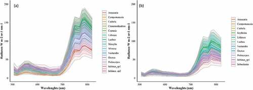
Figure 5 depicts the spectral profile (and standard deviation) with the radiance values of the tree species in the hyperspectral bands. In the bands comprised within the visible region (506–690 nm), there is only a small difference in radiance values of the concerned tree species. Araucaria angustifolia had the lowest radiance values in the entire spectrum for both areas. The discrimination among tree species is more easily achieved in the NIR range (700–819 nm). Nevertheless, even in this region, some groups of species are barely discernible, mainly for Area 1, such as: Araucaria angustifolia, Campomanesia xanthocarpa and Schinus sp1; Podocarpus lambertii, Mimosa scabrella and Ocotea sp.; and Cinnamodendron dinisii and Schinus sp2. For Area 2, three species are clearly distinguishable in this region: Araucaria angustifolia, Sebastiania commersoniana and Schinus sp1, and this explains the higher JM values in the NIR region for this area (Figure 4).

Figure 5. Mean radiance (with standard deviation) of the tree species classified in Area 1 (a) and Area 2 (b).

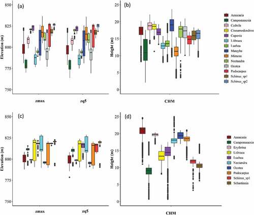
Figure 6 shows the distribution of two PPC features (zmax and zq5) and the CHM values extracted from the samples of each class. It can be noticed that the CHM clearly separates some tree species classes. Campomanesia xanthocarpa presented a lower height in both study areas. In Area 1, besides this species, Mimosa scabrella, Luehea divaricata and Lithraea brasiliensis can be discriminated from other species due to their lower heights. In Area 2, even more species can be differentiated with the CHM, and this justifies the higher importance value assigned to this feature in this area.

Figure 6. Boxplots showing the distribution of the PPC (zmax and zq5) and CHM values of the tree species samples in Area 1 (a and b) and Area 2 (c and d). The central lines within each box are the medians. The boxes edges represent the upper and lower quartiles. Outliers are plotted individually.

In the feature selection using the SFFS method associated with the JM distance, 46 features were selected for Area 1, containing all the groups of generated features: 18 of the 25 VNIR bands corresponding to different regions of the spectrum, all the PPC features, the CHM, 7 MNFs, 10 textural features and all the VIs. For Area 2, 49 features were selected: 21 VNIR bands, all the PPC features, the CHM, 4 MNFs, 3 VIs and 14 textural features.

Classification results

The classification results employing different datasets, classifiers and approaches are presented in Table 5. For Area 1, the best general result was achieved by the CNN classifier associated with the VNIR dataset (OA of 84.37% and Kappa of 0.82). The second best result for this area was reached when the MV rule approach was applied to the SVM classification associated with the VNIR_CHM_PPC_VI dataset (OA of 82.52% and Kappa of 0.80). For Area 2, the opposite occurred: the best general result was achieved after the MV approach was applied to the SVM classification using the VNIR_CHM dataset (OA of 75.47% and Kappa of 0.72), while the second best result was reached by the CNN algorithm associated with the VNIR dataset (OA of 74.95% and Kappa of 0.71).

Table 5. Classification results according to the area/classifier/dataset/approach. The best result for each classifier/approach is highlighted.

		Area 1		Area 2
Classifier	Dataset	OA (%)	Kappa	OA (%)	Kappa
SVM	VNIR	62.67	0.57	48.91	0.41
	VNIR_CHM	67.90	0.63	63.93	0.58
	VNIR_PPC	68.61	0.64	51.50	0.44
	VNIR_CHM_PPC	76.04	0.73	63.10	0.57
	VNIR_CHM_PPC_MNF	76.55	0.73	62.35	0.57
	VNIR_CHM_PPC_GLCM	74.56	0.71	61.98	0.56
	VNIR_CHM_PPC_VI	77.66	0.74	62.94	0.57
	VNIR_CHM_PPC_MNF_VI	77.10	0.74	62.25	0.56
	VNIR_MNF_GLCM_VI	61.91	0.56	47.34	0.39
	MNF_CHM_PPC	68.97	0.64	56.47	0.50
	MNF_CHM_PPC_VI	73.60	0.70	59.06	0.53
	FSJM	74.68	0.71	57.66	0.52
	full	72.59	0.68	61.90	0.56
	MV best SVM result for each area*	82.52	0.80^1	75.47	0.72^1
	OBIA (VNIR_CHM_PPC_VI)	73.52	0.69	-	-
RF	VNIR	59.24	0.52	48.60	0.40
	VNIR_CHM	66.06	0.60	66.02	0.61
	VNIR_PPC	51.46	0.44	63.43	0.58
	VNIR_CHM_PPC	55.91	0.50	65.45	0.60
	VNIR_CHM_PPC_MNF	57.54	0.52	65.94	0.60
	VNIR_CHM_PPC_GLCM	56.60	0.50	66.51	0.61
	VNIR_CHM_PPC_VI	55.59	0.49	65.61	0.60
	VNIR_CHM_PPC_MNF_VI	56.71	0.51	66.21	0.61
	VNIR_MNF_GLCM_VI	59.17	0.52	48.97	0.40
	MNF_CHM_PPC	52.72	0.46	61.72	0.56
	MNF_CHM_PPC_VI	53.82	0.47	63.28	0.57
	FSJM	56.32	0.50	52.08	0.46
	full	57.74	0.52	67.37	0.62
	OBIA(VNIR_CHM_PPC_VI_MNF)	68.00	0.63	-	-
wSVM	VNIR	56.42	0.51	48.98	0.42
	VNIR_CHM_PPC	74.37	0.71	65.15	0.60
	best SVM result for each area*	75.03	0.72	65.60	0.60
CNN	VNIR	84.37	0.82^1	74.95	0.71^1
	VNIR_CHM_PPC	77.17	0.74	70.36	0.65
	VNIR_CHM	79.19	0.76	73.12	0.69^1

*Majority vote (MV) procedure and the wSVM classifier applied to the VNIR_CHM_PPC_VI dataset in Area 1 and the VNIR_CHM dataset in Area 2. ¹Best results that do not significantly differ among themselves according to the z test.

When the pixel-based approaches were compared, the CNN classifier reached the best results for both areas. The SVM classifier had a significant superior performance than the RF in Area 1. On the other hand, it was slightly inferior to the RF in Area 2. The OBIA approach (only applied to Area 1) using the SVM algorithm presented an inferior accuracy as compared with the SVM adopting a pixel-based classification. In its turn, the RF classifier had a slight increase in OA with OBIA when compared with the per-pixel RF classification. The wSVM had a superior performance than the conventional SVM only in Area 2.

Figure 7 illustrates the increase (or decrease) in OA when different features were added, and different approaches were employed for the SVM and RF methods in relation to the classifications using the VNIR dataset with the per-pixel approach. It is possible to notice that the performance of the classifiers varied according to the dataset and study area. Except for the RF applied to Area 1, the inclusion of the CHM and PPC features led to an increase between 13% and 17% in relation to the VNIR dataset. For Area 1, the SVM associated with the VNIR_CHM_PPC_VI dataset reached the best result, with an increase of 15% in relation to the VNIR dataset. The same increase (15%) was observed for the SVM in Area 2 in relation to the VNIR dataset when the VNIR_CHM and VNIR_CHM_PPC datasets were employed.

Figure 7. Differences in overall accuracy with the inclusion of features and approaches in relation to the VNIR dataset, using the SVM and RF classifiers.

For the RF classifier in Area 1, the best result was achieved using the VNIR_CHM, with an increase of 7% in OA in relation to the VNIR dataset. When the OBIA approach was employed, the increase in relation to the pixel-based classification using the VNIR dataset was about 9%, 2% more than the per-pixel approach. In Area 2, the full dataset brought an increase of 19% in relation to the VNIR dataset. The inclusion of other hyperspectral features (i.e. VI, MNF and GLCM) to the VNIR dataset did not significantly change the results in both areas for neither the RF nor SVM classifiers.

When the best per-pixel classification result of the SVM algorithm was aggregated into segments using the MV rule, it was observed a marked increase of 20% and 27% in relation to the VNIR dataset results for Areas 1 and 2, respectively. Comparing the MV and the pixel-based classifications using the same datasets (VNIR_CHM_PPC_VI for Area 1, and VNIR_CHM for Area 2), the increase was nearly 5% and up to 11%, respectively. Contrary to machine learning classifiers, the addition of the CHM and PPC features to the VNIR dataset led to a decrease of approximately 7% and 4.5% in OA of both areas when the CNN classifier was employed.

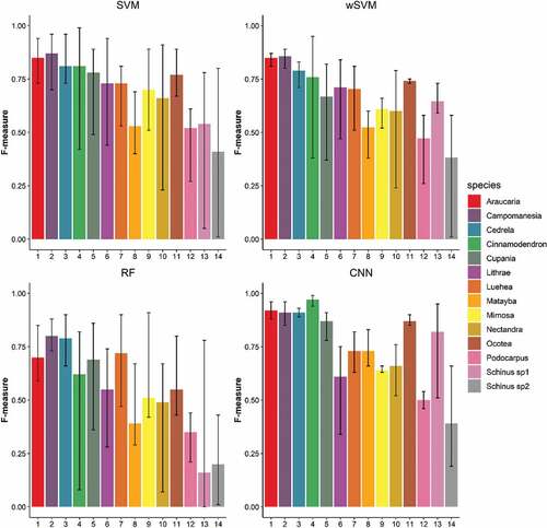
Figure 8 shows the average F-measure of each tree species and classifier in Area 1. The black bars indicate the minimum and maximum F-values, which varied according to the dataset used by each classifier. As expected, the tree species were not equally classified, and some of them presented more variability in the F-measure values when different datasets/classifiers were employed. Regarding the classifiers, it can be observed that the RF presented higher variability in the F-measure results for most species as compared with other classifiers. Generally, classes with fewer samples presented more variability in accuracy, as Cinnamodendron dinisii and both Schinus classes. In the case of the CNN, however, species as Cinnamodendron dinisii, Araucaria angustifolia, Campomanesia xanthocarpa, Cedrela fissilis, Mimosa scabrella, Ocotea sp. and Podocarpus lambertii presented very low variability in the F-measure values, even when the dataset was altered. The CNN presented the best result for nine of fourteen tree species, with the F-measure varying between 0.8 and 1 for most of them. For Lithraea brasiliensis, Nectandra megapotamica, Podocarpus lambertii and Schinus sp2, the SVM and wSVM were the best classifiers, reaching similar results. The RF classifier achieved the highest accuracy for Mimosa scabrella. This classifier had the lowest performance for this area, with some species presenting F-measures below 0.5 even for the best dataset, as Podocarpus lambertii and Schinus sp2.

Figure 8. F-measures of each tree species class for Area 1 according to the classifier. Black bars indicate the minimum and maximum values varying according to the employed dataset.

The confusion matrices of Area 1 (Figure 10) show that the inclusion of the PPC features helped to differentiate some particular classes when the SVM was employed. In the datasets without the PPC features and the CHM, the main confusion among the species occurred with Schinus sp2, which was wrongly assigned to other classes, such as Podocarpus lambertii, Cupania vernalis and Cedrela fissilis, and had other classes incorrectly assigned to it: Cinnamodendron dinisii, Matayba elaeagnoides and Nectandra megapotamica. In these datasets, it also can be noticed that Nectandra megapotamica and Matayba elaeagnoides were incorrectly classified as Ocotea sp., and Nectandra megapotamica and Matayba elaeagnoides were confused with each other. These confusions were generally reduced when the PPC features and the CHM were included to the datasets, but Schinus sp1 was incorrectly classified as Mimosa scabrella, what explains the decrease in the F-measure of that species in comparison with the use of the VNIR_CHM dataset. The wSVM had a similar behavior to the SVM, with the difference that Schinus sp1 presented an increase in the F-measure with the VNIR_CHM_PPC_VI dataset.

Figure 9 shows the average, minimum and maximum F-measures for each tree species in Area 2 according to the classifier. It was observed that most tree species classes had a lower accuracy as compared with Area 1, many of them with F-measures lower than 0.6. For Area 2, the RF classifier reached a general better performance than the SVM, mainly for some tree species, such as Campomanesia xanthocarpa, Nectandra megapotamica and Podocarpus lambertii. In this area, the wSVM classifier had a better performance than the conventional SVM, which was more evident for some classes, like Campomanesia xanthocarpa, Cedrela fissilis and Erythrina falcata. The CNN classifier outperformed other classifiers, presenting F-measures over 0.8 for many classes and less variability in F-measures accuracies. However, it totally misclassified the species Campomanesia xathocarpa. Again, the RF presented more variability in the F-measure values.

Figure 9. F-measures of each tree species class for Area 2 according to the classifier. Black bars indicate the minimum and maximum values varying according to the dataset.

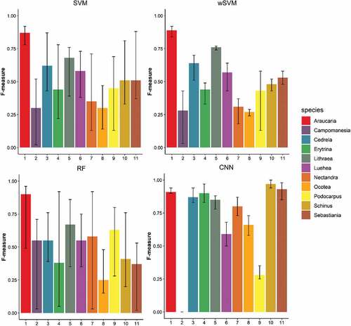
Figure 10. Some of the confusion matrices of Area 1 (top) and Area 2 (bottom). Note: Classes identified according to the species ID presented in .Table 2

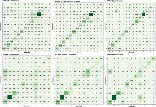
Similarly to Area 1, almost all the tree species presented an increase in F-measures when the CHM and PPC features were added to the VNIR dataset with the SVM, wSVM and RF classifiers. In the confusion matrices of the VNIR dataset (Figure 9), it can be noticed that Podocarpus lambertii was wrongly assigned to a lot of different species, such as Ocotea sp., Cedrela fissilis, Campomanesia xanthocarpa and Araucaria angustifolia, while Luehea divaricata was wrongly assigned to Podocarpus lambertii. Campomanesia xanthocarpa was wrongly classified as Lithraea brasiliensis and Luehea divaricata when only the VNIR bands were used. The incorporation of the CHM and PPC features markedly reduced the confusion among these classes in machine learning classifiers. Again, except for Cedrela fissilis and Araucaria angustifolia, all the tree species presented a decrease between 0.01 and 0.13 in F-measures when the PPC or the CHM were included in the CNN classifier.

In Area 2, both methods dealing with imbalanced sample sets (CNN and wSVM) were more accurate for some tree species. The CNN achieved the best result for seven of the eleven tree species, particularly for six classes, namely Cedrela fissilis, Erythrina falcata, Nectandra megapotamica, Ocotea sp., Schinus therebinthifolius and Sebastiania commersoniana. The wSVM had an equal or better performance than the conventional SVM in all the classes. Classes with fewer samples, such as Campomanesia xanthocarpa and Erythrina falcata, had a more pronounced accuracy increase when the wSVM was employed. For the former one, the F-measure increased from 0.35 to 0.40, while for Erythrina falcata it rose up from 0.44 to 0.49. In this area, the wSVM reached a better performance even for classes with more samples, as Podocarpus lambertii and Araucaria angustifolia. The wSVM not only gives different weights to each class, but also to each sample. In this case, if one sample is not regarded as robust, i.e. is not close to the class cluster, it will receive a smaller weight. Thus, this algorithm can improve the accuracy of majority classes as well.

Species maps

Figure 11 shows the classification images considering each ITC sample of Area 1 (training and test sets). The classified images were produced in order to see the proportion of pixels correctly labeled within each ITC, and if the species were detected by the classification method. The proposed approach produced reliable results considering only the ITCs checked in the field.

Figure 11. Examples of classification images for Area 1. a) Reference samples; b) the SVM classifier (VNIR_CHM_PPC dataset) after the MV rule – the red circle shows missing ITCs of Podocarpus; c) OBIA associated with the RF classifier and the VNIR_CHM_PPC_VI_MNF dataset – the red circle shows two missing ITCs of Nectandra and one of Podocarpus; d) the CNN classifier with the VNIR dataset – the red circle shows one missing ITC of Nectandra.

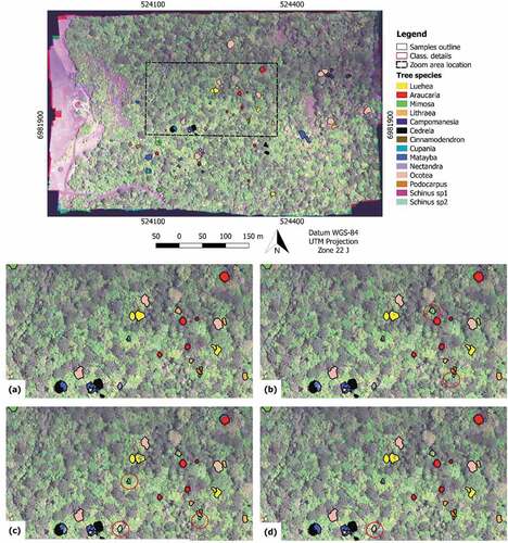
In general, the methods detected the species and assigned the correct class to the ITCs. However, in some cases, only few pixels inside the ITCs were correctly classified, meaning that the method detected the species, but did not classify all the ITC accordingly. In other minor cases, all the ITC was misclassified, which was mainly observed for the small-sized ones.

Discussion

Considerations about variable importance and tree species classification using machine learning methods

This study showed that the incorporation of the CHM and PPC features with the VNIR bands significantly increased the classification accuracies when machine learning methods were applied (RF, SVM and wSVM). One of the pioneer studies exploring the use of UAV-based photogrammetric and hyperspectral imagery for tree species classification was made by Nevalainen et al. (2017), in which they reached 95% of OA. One year later, Tuominen et al. (2018) reported an increase of 0.07 in the Kappa index (Kappa of 0.77) when 3D features were incorporated into UAV-borne hyperspectral data to classify 26 tree species in an arboretum located in Finland. Despite their optimistic results, none of the aforementioned studies involved tropical environments. While Nevalainen et al. (2017) only classified four tree species in a boreal forest, the study of Tuominen et al. (2018) was carried out in an arboretum area with tree species distributed in homogeneous stands, what eases their recognition both at a stand and individual tree level.

So far, very few studies explored the combination of 3D information with hyperspectral data for tree species classification in (sub)tropical forests, although the benefits of this integration have long been emphasized (Fassnacht et al. 2016). Shen and Cao (2017) reached an improvement of 5.6% (OA of 89.3%) when using both hyperspectral and airborne LiDAR features to classify five tree species in a subtropical forest using the RF algorithm. Sothe et al. (2019a) reported that the inclusion of PPC features to the hyperspectral bands increased the OA by 11% (OA of 72.4%) when classifying 12 tree species in a subtropical forest area. In another highly diverse environment, Piiroinen et al. (2017) found an increase of 6% (OA of 57%) when LiDAR features were added to the hyperspectral bands for classifying 31 tree species in a diverse African agroforestry using the SVM method.

Similarly to the abovementioned studies, the incorporation of 3D information derived from PPC data was also more evident for some species, such as Schinus sp2, Ocotea sp., Nectandra megapotamica and Matayba eleaeagnoides in Area 1. Ocotea sp. class comprises two species of Ocotea genus (O. pulchella and O. puberula), leading to a higher variance in their spectral response. Moreover, Ocotea sp. and Nectandra megapotamica belong to the same family (Lauraceae), which grants them similar spectral characteristics. In this case, the inclusion of the PPC features can tackle the spectral similarity among these tree species. The PPC features may also capture differences in the crown structure of Matayba elaeagnoides and Ocotea sp., since the former one has a wider top with irregular branching, while the latter one has a smaller and rounded top (Lorenzi 1992). For Area 2, where the VNIR dataset was used with machine learning methods, most of the confusion was associated with Podocarpus lambertii. This species is a conifer and presents irregular or cuneiform crowns. These structure differences were able to help in discriminating it from other broadleaves species when the PPC features were incorporated into the models.

The inclusion of the height information (CHM) improved the accuracies from 5% to 7% for Area 1, and from 15 to 17% for Area 2. Indeed, the CHM was more important than the PPC features for Area 2, which may be due to the lower PPC density of this area, besides particularities of it and its individual trees. These findings comply with the studies of Cho et al. (2012), Naidoo et al. (2012) and Asner et al. (2008), who also pointed out the tree height as an important variable for tree species classification. In tropical forests, this variable can be useful to discriminate species belonging to different successional groups, such as pioneer, secondary and climatic, since they may have different heights according to their capacity to adjust to differentiated lighting levels (Boardman 1977). In Area 1, there was a great confusion between Schinus sp1 and Mimosa scabrella, and between the latter one and Podocarpus lambertii in the datasets without the CHM information. These three species belong to different successional groups: Schinus sp1 and Mimosa scabrella are considered pioneer species, while Podocarpus lambertii is a late secondary or climatic shade-tolerant species (Lorenzi 1992). As a shade-tolerant species, Podocarpus lambertii can live under the shadow of other trees, and hence, might present a smaller height. Despite the fact that both are pioneer species, Mimosa scabrella and Schinus sp1 have different heights (Figure 6), which can be due to particularities of the area. For instance, it was verified that Mimosa scabrella samples were located near the road or clearing areas. The lack of competition for light could have caused their limited growth in height. On the other hand, Schinus sp1 samples were found in the middle of the forest, which could have led to their high growth rate, as this species searches for light. For this reason, when the height information was incorporated, there was an increase in classification accuracies of these species.

Araucaria angustifolia, the most frequent species in both study areas, maintained stable accuracies even with the inclusion of PPC features. It can be observed in Figure 5 that this species presents the lowest radiance values in the VNIR bands, being more easily discriminated from other species. In this case, the higher absorption of the needle structure of Araucaria angustifolia reduces its spectral response in the NIR range when compared to broadleaves species (Roberts et al. 2004). Conversely, Podocarpus lambertii, another conifer found in the study areas, tended to present more confusion with some broadleaves species, especially when the VNIR dataset was used. This may have occurred because of its particular branch structure that led to confusion with broadleaves species with small leaves, such as Mimosa scabrella in Area 1, even with the inclusion of the PPC features.

For both areas, the use of the MV rule significantly increased the accuracy of the pixel-based classification (between 5% and 11%), while the OBIA approach (only applied to Area 1) did not produce significant difference. These findings corroborate other studies that compared tree species classification using pixel-based and MV approaches (Clark, Roberts, and Clark 2005; Dalponte et al. 2013, 2014; Ferreira et al. 2016), and also further studies comparing these two approaches with OBIA (Clark and Roberts 2012; Féret and Asner 2013). Clark and Roberts (2012) compared the OBIA approach, composed by the mean spectra of each ITC, to per-pixel and MV approaches. The pixel-based classification had roughly the same performance (nearly 70% of OA) to the one achieved when using the average spectra from ITCs in OBIA, however, when applying the MV, the accuracy surprisingly rose to 87%. Féret and Asner (2013) reached better results when using the MV approach (83.6% of OA), followed by the OBIA approach (79.6% of OA) and lastly the per-pixel classification (74.9% of OA), when classifying tree species in a tropical forest. However, when employing the MV and OBIA classifications, there was a reduction in the classes number from 17 to 10, due to the small number of pixels and ITCs labeled to train the classifiers. Furthermore, likewise our study, the authors pointed out that the segmentation did not delineate ITCs correctly, but each crown was instead composed by several segments.

According to Clark and Roberts (2012), by applying the MV rule to pixels within ITCs, the error from misclassified pixels within a crown is minimized, what leads to higher accuracies. However, in this approach, the ITCs may have high internal spectral variability, since they can receive the correct species label with only a fourth of the correctly classified pixels. Thus, OBIA can be a better alternative to deal with the spectral variability within the classes, which is common when high spectral resolution data are used, but in this case more ITC samples are needed. Furthermore, shadow, underlying objects, and other materials within an ITC may decrease the purity of its extracted spectra and further reduce classification accuracy (Liu and Wu 2018). Concerning this, Liu and Wu (2018) proposed a pixel weighting approach in which they extract the illuminated-leaf fraction at each pixel using a spectral mixture analysis (SMA) model and then calculate the ITC spectra using the illuminated-leaf fractions as weights.

For Area 1, all the VNIR bands showed similar importance according to the JM distance. Only slightly higher importance values can be noticed for the first two bands (506 to 519 nm), and four bands between 659 and 690 nm. These regions included the green peak and the chlorophyll absorption features and contain useful information for the discrimination of tree species with hyperspectral data (Naidoo et al. 2012; Fassnacht et al. 2014; Ferreira et al. 2016). The NIR bands, regarded as an important region for the purpose of tree species classification (Clark and Roberts 2012; Dalponte, Bruzzone, and Gianelle 2012; Piiroinen et al. 2017), were not relevant for Area 1, while for Area 2 these bands had the highest JM values. This region is mostly influenced by the structure of the tree (Ponzoni, Shimabukuro, and Kuplich 2012), therefore, the changes in the viewing angle may mask the relative spectral differences among the species (Nevalainen et al. 2017). Unfortunately, the limited spectral range of the FPI camera (500–900 nm) did not allow for evaluating the discrimination among the tree species in the SWIR region. Ferreira et al. (2016) reported a significant increase in accuracy (14%) when including SWIR bands for tree species classification. Tuominen et al. (2018) reached the best result when combining VNIR and SWIR bands with 3D features extracted from the PPC. Nevertheless, their second-best result was achieved using only VNIR bands and 3D features, suggesting that these features can somehow compensate for the lack of SWIR data.

In fact, the CHM and PPC features were markedly more important than the hyperspectral features (i.e. VI, MNF and GLCM features). The use of all the VNIR bands, hyperspectral features, the CHM and PPC features in the full dataset did not improve the accuracy when compared with the use of the VNIR_CHM_PPC dataset (except for the RF in Area 2). The replacement of the VNIR bands by the MNF features (MNF_CHM_PPC dataset) led to a decrease from 2.34% to 7% in OA when considering both areas and the SVM and RF classifiers. Some studies reported an improvement when MNF components were used instead of spectral bands, but it is worth stressing that they dealt with more than 100 spectral bands (e.g, Ghosh et al. 2014; Piiroinen et al. 2017). In this situation, the MNF transformation was a reliable approach to reduce the dimensionality and redundancy inherent to high spectral resolution data, reaching better accuracies (Ghosh et al. 2014). The same consideration can be made regarding the FS process, in which 46 of the original 68 features were selected for Area 1, and 49 for Area 2, resulting in a non-significant difference in accuracy when compared with the full dataset for both areas. Piiroinen et al. (2017) reported that the FS process had only a small impact on tree species classification accuracies, but they highlighted its importance in achieving the same level of accuracy with a smaller number of input features.

Regarding the classifiers, the SVM clearly outperformed the RF for Area 1, but it was worse than the RF in Area 2. Studies comparing both methods for tree species classification indicated that the SVM had a similar (Ghosh et al. 2014; Ballanti et al. 2016) or superior performance than the RF (Dalponte, Bruzzone, and Gianelle 2012; Deng et al. 2016; Ferreira et al. 2016; Piiroinen et al. 2017; Raczko and Zagajewski 2017). Some studies reported that the SVM performs better than the RF in the presence of small or imbalanced sample sets because the latter classifier focuses on the prediction accuracy of the majority classes (Chen et al. 2004; Dalponte, Bruzzone, and Gianelle 2012). However, this was not verified in this study, since Area 2 also presents a small and imbalanced sample set, and the RF was superior to the SVM in that case. Piiroinen et al. (2017) observed that the fusion of LiDAR features with MNF components significantly improved the accuracy for the SVM algorithm, while for the RF classifier there was not statistically significant improvement between these datasets. Similar behavior was reported by Deng et al. (2016), when comparing the SVM and RF algorithms for tree species classification. They observed more accuracy gain when features were added to the SVM classifier instead of the RF. In this study, the RF performance decreased with the addition of other features, including the PPC features, for the VNIR_CHM dataset in Area 1, but it remained relatively stable in Area 2. In such situations, the impact of data fusion depends on the classifier (Piiroinen et al. 2017) and, in our case, also on the study area peculiarities. In fact, it is difficult to keep the generalization of the classification process when changing the datasets and study areas, and this is one of the reasons underlying the findings of Fassnacht et al. (2016), who reported the importance of integrating more than a single test site in any comparative study on tree species classification.

The wSVM outperformed the SVM only in Area 2. Since the wSVM assigns different weights to different classes (or samples), it forces the new separating hyperplane to pay more attention to the minority classes samples (Nguyen, Demir, and Dalponte 2019), which are more remarkable in this area. Another fact to consider is that besides the class, this algorithm also assigns different weights to each sample. Area 2 presents larger coregistration errors among the bands than Area 1, thus non reliable pixel samples, e.g., those situated on the border of ITCs where these errors can be more noticeable, and hence may receive a lower weight in the classification process. In fact, it was verified that for Area 2, even classes with more samples had an increase in accuracy when the wSVM was applied.

Another fact to consider is about the classifier parameters. Although all the machine learning classifiers have parameters to be optimized, the parameter values used in this work provided an output similar or even more accurate when compared with other studies (e.g., Dalponte, Bruzzone, and Gianelle 2012; Immitzer, Vuolo, and Clement Atzberger 2016; Raczko and Zagajewski 2017). In this sense, studies investigating the parameterization for SVMs showed contradictory results. Melgani and Bruzzone (2004) and Maxwell, Warner, and Fang (2018) both found SVMs to be robust to parameter settings. Conversely, Foody and Mathur (2004) and Trisasongko et al. (2017) found larger impact on classification accuracies, with differences up to 20% when varying the SVM parameters. On the other hand, RF has generally been found to be robust to parameter settings (Rodriguez-Galiano et al. 2012; Trisasongko et al. 2017; Trisasongko and Paull 2019; Maxwell, Warner, and Fang 2018). Maxwell, Warner, and Fang (2018) reported that if optimization cannot be performed, using the default value for the parameter “number of variables” and selecting a large number of trees (e.g., 500) appears to produce a classification accuracy close to what can be achieved by means of optimization. Finally, these authors suggest that machine learning may still outperform parametric classifiers, such as maximum likelihood, even with little effort to tune the classification parameters.

Considerations about tree species classification using the CNN

The CNN classifier outperformed machine learning classifiers for both areas, reaching the best performance when the VNIR dataset was used. Conversely, machine learning methods had a poorer performance when only the VNIR bands were employed. As stated by Li, Zhang, and Shen (2017) and Gao, Lim, and Jia (2018), the main advantage of deep learning methods, as CNN, is that they can extract spatial and spectral features automatically from the original images, learning features during training, with minimal prior knowledge about the task.

When machine learning classifiers were associated with the MV approach, they reached a performance similar to the CNN in both areas. The MV rule includes spatial context when aggregates the pixels into segments, leading to higher accuracies and reducing the “salt and pepper” effect in classifications. In the case of the CNN, it can be observed that the classification images, even without the further use of segments (MV), were more homogeneous and tended to correct a larger proportion of pixels inside the ITCs than the pixel-based classifications using machine learning methods. This can be associated with the contextual window (patch sizes) used for the features reckoning, which considers the information on the pixel neighborhood. In the case of trees, the spatial structure of canopies is related to the tree size: if a pixel falls in a specific tree, its neighbors are also likely to be in the same tree and have similar information. Information in neighboring pixels is related to the information in a focal pixel and these relationships decay with distance. CNN classifiers operate according to such principle of detecting patterns in groups of nearby pixels and relating them to “background” information (Li, Zhang, and Shen 2017; Fricker et al. 2019).

Another fact to consider is that besides the need of ITC segments in an MV rule approach, more features were necessary in machine learning methods to reach similar accuracies to those attained by the CNN. Indeed, contrary to machine learning methods, the CNN presented a decrease in accuracy for most classes when the PPC, the CHM or both were included in the dataset. This can be ascribed to the fact that these features were manually extracted before their inclusion in the algorithm. As a CNN automatically extracts its own features, the inclusion of the raw PPC instead of rasterized features could enable the extraction of more useful features by this algorithm. A similar behavior was observed by Sothe et al. (2019b) when comparing CNN and ensemble methods using WV-2 data, LiDAR features, and their integration. Despite the difference was very small, the CNN had the best performance when the WV-2 data were employed using only the spectral bands; and the worst accuracy when only LiDAR features were used. However, in that case, even for the CNN, an increase in accuracy was observed when LiDAR features were integrated into the WV-2 data, which can be due to the presence of intensity features of LiDAR, and not the elevation ones. Hartling et al. (2019) also reached the best OA for a dense CNN when multispectral bands of WV-3 were employed together with LiDAR data, but they used only the intensity image instead of elevation features.

According to He et al. (2018), most of the existing methods do not extract informative features from LiDAR-derived rasterized data in a deep manner. Hamraz et al. (2018) pointed out that LiDAR point clouds are not easily processed by the human visual system, and hence the expert-designed features may as well be suboptimal and likely miss useful information. Qi et al. (2016), (2017)) mentioned that 3D data have attracted less attention in view of their more costly acquisition/processing and their less intuitive and less conventional representation formats, which demand non-trivial pre-processing techniques to discretize the data and make them usable for deep learning methods. In this respect, some approaches can be explored in future works, such as voxel spaces to create representations that can drive and be processed by a 3D CNN (Maturana and Scherer 2015; Wu et al. 2015; Guan et al. 2019) or even the use of morphological and multiattribute profiles to extract information from LiDAR data (He et al. 2018).

Until the present moment, there are few studies exploring CNN for tree species classification purposes (Pölönen et al. 2018; Fricker et al. 2019; Guan et al. 2019; Hartling et al. 2019). Pölönen et al. (2018) reached 96.2% of OA when classifying three tree species of a boreal forest using a 3D CNN and hyperspectral data, while Guan et al. (2019) reached 96.4% of OA when classifying 10 tree species using mobile LiDAR data and a 3D CNN in an urban environment. Such high OA values are usually associated with validation samples internally generated by the CNN during training. Hartling et al. (2019) compared a dense CNN architecture to the RF and SVM methods to classify eight tree species in an urban area using WV-2, WV-3 and LiDAR data. In their study, the CNN classifier reached 82.6% of OA in comparison to 60% achieved by machine learning methods. Fricker et al. (2019) reached an F-score of 0.87 when classifying seven tree species in a mixed-conifer forest in USA. Our results are comparable to those of the above reported works, given that Pölönen et al. (2018) and Fricker et al. (2019) handled a limited number of species in boreal or temperate regions and both Guan et al. (2019) and Hartling et al. (2019) dealt with urban areas, which represent a more controlled environment. Likewise our study, Hartling et al. (2019) emphasized the ability of the CNN in extracting information from the input dataset and pointed out that the addition of features, such as VIs and texture, tended to decrease the OA of the CNN.

Although outperforming other methods for the majority of the analyzed tree species in both areas, the CNN totally misclassified Campomanesia xanthocarpa in Area 2. Even so, their training samples were correctly classified, which can be a specific case of overfitting, since different ITCs were used as test samples to evaluate the methods.

The non-dependence of former steps of feature extraction and segmentation before the classification makes CNN an attractive solution for tree species classification in highly diverse environments, even in the presence of small sample sets, if a data augmentation process is applied. On the other hand, the processing time and computer power requirements are the biggest disadvantages of such method. Huang et al. (2002) noted that the higher accuracy of artificial neural networks (ANNs) algorithms compared to decision trees was offset by the larger computational cost. However, when considering the VNIR dataset and the pixel-based approach, this study showed that the CNN reached accuracies between 22% and 26% higher than the RF and SVM for both areas, which can counterbalance the price of its high computational cost.

Conclusion

This study explored the ability of UAV-based PPC and UAV-hyperspectral data for tree species classification using machine learning methods and a deep learning algorithm in two subtropical forest fragments. The inclusion of the PPC features and the CHM enabled a great increase in accuracy in tree species classification results when machine learning methods were applied (SVM, wSVM and RF), between 13 and 17% depending on the classifier and the study area. However, a decrease was observed when these features were included in the classification with a deep learning method (CNN).

The OBIA approach (only applied to Area 1) did not increase the OA for the SVM, while a slight increase was observed for the RF algorithm in comparison with the other pixel-based classifications. When the per-pixel classifications were aggregated into segments through an MV rule, it was observed a marked increase in accuracy for both study areas (5% for Area 1 and 11% for Area 2), considering the same datasets individually. This can be explained by the fact that this procedure reduced the classification errors associated with the spectral variability of high spatial resolution data.

The wSVM, a new SVM approach to deal with imbalanced sample sets and unreliable samples, improved the accuracy not only for some lesser represented classes, but for some major classes in Area 2 as well. The use of a CNN architecture associated with a previous step aiming to balance the sample sets was also successful to classify tree species in both areas, since the method outperformed all the other algorithms in comparison with pixel-based approaches.

In fact, the CNN outperformed machine learning methods without the need of relying on segmentation or making use of hand-engineered features. The method reached an OA of 84.4% in Area 1 and 74.95% in Area 2, when using the VNIR bands alone, and it is nearly 22% to 26% more accurate than the SVM and RF classifiers when considering the VNIR dataset. In both areas, when the best dataset result of the SVM classifier was incorporated into segments by means of the MV rule, it reached a comparable performance to that of the CNN. However, not only the segments but also the use of the PPC features and the CHM were of great relevance to increase the accuracy.

This work indicated that the adopted approaches for the semiautomatic classification of 16 tree species in two fragments of a subtropical portion of the Atlantic Rain Forest may be promising. The methodology can be useful to assist the conservation of this severely threatened biome, optimizing the monitoring of its forest biodiversity. Furthermore, the methodology can be used to classify specific tree species, such as the endangered ones, like Araucaria angustifolia and Cedrela fissilis. In further studies, a feasible approach for improving the classification performance is envisaged to explore ITC delineation methods for tropical forest environments, combining PPC and hyperspectral data. This proper delineation can be associated with an OBIA classification at an ITC level. Moreover, increasing the number of ITC samples in a way to enable a more robust model and consistent classification is also a goal to be pursued. The generalization of the classification is another point to consider, since the use of two study areas, instead of one, showed that the particularities of each area should be duly taken into account when choosing the most reliable features and algorithms for the purpose of classifying tree species. Therefore, it is recommended that other areas be tested for more conclusive results.

Finally, it is also necessary to explore methods involving the extraction of deep features directly from the PPC using the CNN classifier. This algorithm showed a great potential for classifying tree species employing the VNIR bands alone, but it did not benefit from the PPC features manually extracted before the classification. It is believed that this algorithm can perform even better in case a more robust way to extract 3D features be implemented.

Acknowledgements

We gratefully acknowledge the financial support offered to this research by the Coordination for the Improvement of Higher Education Personnel (CAPES) (Grants Nr. 88881.190545/2018-01; 88882.330700/2018-01); the Brazilian National Council for Scientific and Technological Development (CNPq) (Grants Nr.153854/2016-2; 303523/2018-2; 303670/2018-5; 313887/2018-7; 436863/2018-9); the Foundation for Support of Research and Innovation, Santa Catarina State (FAPESC) (Grant Nr. 2017TR1762); the Sao Paulo Research Foundation (FAPESP) (Grant Nr. 13/50426-4); and FAPESC/CAPES (Grant Nr. 88887.178653/2018-00).

Disclosure statement

No potential conflict of interest was reported by the authors.

Additional information

Funding

This work was supported by the Conselho Nacional de Desenvolvimento Científico e Tecnológico [303670/2018-5];Conselho Nacional de Desenvolvimento Científico e Tecnológico [436863/2018-9];Conselho Nacional de Desenvolvimento Científico e Tecnológico [313887/2018-7];Conselho Nacional de Desenvolvimento Científico e Tecnológico [303523/2018-2];Conselho Nacional de Desenvolvimento Científico e Tecnológico [153854/2016-2];Coordenação de Aperfeiçoamento de Pessoal de Nível Superior [88887.178653/2018-00];Coordenação de Aperfeiçoamento de Pessoal de Nível Superior [88882.330700/2018-01];Coordenação de Aperfeiçoamento de Pessoal de Nível Superior [88881.190545/2018-01];Fundação de Amparo à Pesquisa do Estado de São Paulo [13/50426-4];Fundação de Amparo à Pesquisa e Inovação do Estado de Santa Catarina [2017TR1762].

References

- Aasen, H., E. Honkavaara, A. Lucieer, and P. J. Zarco-Tejada. 2018. “Quantitative Remote Sensing at Ultra-High Resolution with UAV Spectroscopy: A Review of Sensor Technology, Measurement Procedures, and Data Correction Workflows.” Remote Sensing 10 (7): 1091. doi:10.3390/rs10071091.
- Abadi, M., A. Agarwal, P. Barham, E. Brevdo, Z. Chen, C. Citro, G. S. Corrado, et al. 2015. TensorFlow: Large-scale Machine Learning on Heterogeneous Systems. Available at: tensorflow.org. Accessed 6 Aug 2018.
- Andrade, A. C., C. N. Francisco, and C. M. Almeida. 2014. “Desempenho De Classificadores Paramétrico E Não Paramétrico Na Classificação Da Fisionomia Vegetal.” Revista Brasileira De Cartografia 66 (2): 349–363.
- Asner, G. P., D. E. Knapp, T. Kennedy-Bowdoin, M. O. Jones, R. E. Martin, J. Boardman, and R. F. Hughes. 2008. “Invasive Species Detection in Hawaiian Rainforests Using Airborne Imaging Spectroscopy and LiDAR.” Remote Sensing of Environment 112 (5): 1942–1955. doi:10.1016/j.rse.2007.11.016.
- Baatz, M., and M. Schäpe. 2000. “Multiresolution Segmentation — An Optimization Approach for High Quality Multi-scale Image Segmentation.” In Angewandte Geographische Informations- Verarbeitung XII, edited by J. Strobl, T. Blaschke, and G. Griesebner, 12–23. Karlsruhe: Wichmann Verlag.
- Baldeck, C. A., G. P. Asner, R. E. Martin, C. B. Anderson, D. E. Knapp, J. R. Kellner, and S. J. Wright. 2015. “Operational Tree Species Mapping in a Diverse Tropical Forest with Airborne Imaging Spectroscopy.” PLoS ONE 10: e0118403. doi:10.1371/journal.pone.0118403.
- Ballanti, L., L. Blesius, E. Hines, and B. Kruse. 2016. “Tree Species Classification Using Hyperspectral Imagery: A Comparison of Two Classifiers.” Remote Sensing 8: 445. doi:10.3390/rs8060445.
- Blackburn, G. A. 1998. “Spectral Indices for Estimating Photosynthetic Pigment Concentrations: A Test Using Senescent Tree Leaves.” The International Journal of Remote Sensing 19 (4): 657–675. doi:10.1080/014311698215919.
- Boardman, N. K. 1977. “Comparative Photosynthesis of Sun and Shade Plants.” Annual Review of Plant Physiology 28: 355–377. doi:10.1146/annurev.pp.28.060177.002035.
- Breiman, L. 2001. “Random Forests.” Machine Learning 45 (1): 5–32. doi:10.1023/A:1010933404324.
- Chen, C., A. Liaw, and L. Breiman, . 2004. Using random forest to learn imbalanced data. USA: Berkeley: University of California.
- Chen, Y., Z. Lin, X. Zhao, G. Wang, and Y. Gu. 2014. “Deep Learning-Based Classification of Hyperspectral Data.” IEEE Journal of Selected Topics in Applied Earth Observations and Remote Sensing 7 (6): 2094–2107. doi:10.1109/JSTARS.2014.2329330.
- Cho, M. A., R. Mathieu, G. P. Asner, L. Naidoo, J. Van Aardt, A. Ramoelo, P. Debba, et al. 2012. “Mapping Tree Species Composition in South African Savannas Using an Integrated Airborne Spectral and LiDAR System.” Remote Sensing of Environment 125: 214–226. doi:10.1016/j.rse.2012.07.010.
- Clark, M. L., and D. A. Roberts. 2012. “Species-level Differences in Hyperspectral Metrics among Tropical Rainforest Trees as Determined by a Tree-based Classifier.” Remote Sensing 4: 1820–1855. doi:10.3390/rs4061820.
- Clark, M. L., D. A. Roberts, and D. B. Clark. 2005. “Hyperspectral Discrimination of Tropical Rain Forest Tree Species at Leaf to Crown Scales.” Remote Sensing of Environment 96: 375–398. doi:10.1016/j.rse.2005.03.009.
- Cohen, J. 1960. “A Coefficient of Agreement for Nominal Scales.” Educational and Psychological Measurement 20 (1): 37–46. doi:10.1177/001316446002000104.
- Colombo, A. F., and C. A. Joly. 2010. “Brazilian Atlantic Forest Lato Sensu: The Most Ancient Brazilian Forest, and a Biodiversity Hotspot, Is Highly Threatened by Climate Change.” Brazilian Journal of Biology 70: 697–708. doi:10.1590/S1519-69842010000400002.
- Dalponte, M., H. O. Ørka, L. T. Ene, L. T., . T. Gobakken, and E. Naesset. 2014. “Tree Crown Delineation and Tree Species Classification in Boreal Forests Using Hyperspectral and ALS Data.” Remote Sensing of Environment 140: 306–317. doi:10.1016/j.rse.2013.09.006.
- Dalponte, M., H. O. Ørka, T. Gobakken, D. Gianelle, and E. Næsset. 2013. “Tree Species Classification in Boreal Forests with Hyperspectral Data.” IEEE Transactions on Geoscience and Remote Sensing 51: 2632–2645. doi:10.1109/TGRS.2012.2216272.
- Dalponte, M., L. Bruzzone, and D. Gianelle. 2012. “Tree Species Classification in the Southern Alps Based on the Fusion of Very High Geometrical Resolution Multispectral/hyperspectral Images and LiDAR Data.” Remote Sensing of Environment 123: 258–270. doi:10.1016/j.rse.2012.03.013.
- Dalponte, M., L. T. Ene, M. Marconcini, T. Gobakken, and E. Næsset. 2015. “Semi-supervised SVM for Individual Tree Crown Species Classification.” ISPRS Journal of Photogrammetry and Remote Sensing 110: 77–87. doi:10.1016/j.isprsjprs.2015.10.010.
- Deng, S., M. Katoh, Y. Xiaowei, J. Hyyppä, and T. Gao. 2016. “Comparison of Tree Species Classifications at the Individual Tree Level by Combining ALS Data and RGB Images Using Different Algorithms.” Remote Sensing 8 (12): 1034. doi:10.3390/rs8121034.
- Fassnacht, F. E., C. Neumann, M. Förster, H. Buddenbaum, A. Ghosh, A. Clasen, P. K. Joshi, and B. Koch. 2014. “Comparison of Feature Reduction Algorithms for Classifying Tree Species with Hyperspectral Data on Three Central European Test Sites.” IEEE Journal of Selected Topics in Applied Earth Observations and Remote Sensing 7 (6): 2547–2561. doi:10.1109/JSTARS.2014.2329390.
- Fassnacht, F. E., H. Latifi, K. Stereczak, A. Modzelewska, M. Lefsky, L. T. Waser, C. Straub, and A. Ghosh. 2016. “Review of Studies on Tree Species Classification from Remotely Sensed Data.” Remote Sensing of Environment 186: 64–87. doi:10.1016/j.rse.2016.08.013.
- Féret, J., and G. P. Asner. 2013. “Tree Species Discrimination in Tropical Forests Using Airborne Imaging Spectroscopy.” IEEE Transactions on Geoscience and Remote Sensing 51: 73–84. doi:10.1109/TGRS.2012.2199323.
- Ferreira, M. P., F. H. Wagner, L. E. O. C. Aragao, Y. E. Shimabukuro, and C. R. Souza Filho. 2019. “Tree Species Classification in Tropical Forests Using Visible to Shortwave Infrared WorldView-3 Images and Texture Analysis.” ISPRS Journal of Photogrammetry and Remote Sensing 149: 119–131. doi:10.1016/j.isprsjprs.2019.01.019.
- Ferreira, M. P., M. Zortea, D. C. Zanotta, Y. E. Shimabukuro, and C. R. Souza Filho. 2016. “Mapping Tree Species in Tropical Seasonal Semi-deciduous Forests with Hyperspectral and Multispectral Data.” Remote Sensing of Environment 179: 66–78. doi:10.1016/j.rse.2016.03.021.
- Foody, G. M., and A. Mathur. 2004. “A Relative Evaluation of Multiclass Image Classification by Support Vector Machines.” IEEE Transactions on Geoscience and Remote Sensing 42 (6): 1335–1343. doi:10.1109/TGRS.2004.827257.
- Franklin, S. E., and O. S. Ahmed. 2017. “Deciduous Tree Species Classification Using Object-based Analysis and Machine Learning with Unmanned Aerial Vehicle Multispectral Data.” International Journal of Remote Sensing 39: 5236–5245. doi:10.1080/01431161.2017.1363442.
- Fricker, G. A., J. D. Ventura, J. A. Wolf, M. P. North, F. W. Davis, and J. A. Franklin. 2019. “Convolutional Neural Network Classifier Identifies Tree Species in Mixed-Conifer Forest from Hyperspectral Imagery.” Remote Sensing 11: 2326. doi:10.3390/rs11192326.
- Fukushima, K. 1980. “Neocognitron: A Self-organizing Neural Network Model for A Mechanism of Pattern Recognition Unaffected by Shift in Position.” Biological Cybernetics 36: 193–202. doi:10.1007/BF00344251.
- Gamon, J. A., J. Peñuelas, and C. B. Field. 1992. “A Narrow-waveband Spectral Index that Tracks Diurnal Changes in Photosynthetic Efficiency.” Remote Sensing of Environment 41: 35–44. doi:10.1016/0034-4257(92)90059-S.
- Gao, Q., S. Lim, and X. Jia. 2018. “Hyperspectral Image Classification Using Convolutional Neural Networks and Multiple Feature Learning.” Remote Sensing 10 (2): 299. doi:10.3390/rs10020299.
- Ghosh, A., E. F. Fassnacht, P. K. Joshi, and B. Koch. 2014. “A Framework for Mapping Tree Species Combining Hyperspectral and LiDAR Data: Role of Selected Classifiers and Sensor across Three Spatial Scales.” International Journal of Applied Earth Observation and Geoinformation 26: 49–63. doi:10.1016/j.jag.2013.05.017.
- Graves, S. J., G. P. Asner, R. E. Martin, C. B. Anderson, M. S. Colgan, L. Kalantari, and S. Bohlman. 2016. “Tree Species Abundance Predictions in a Tropical Agricultural Landscape with a Supervised Classification Model and Imbalanced Data.” Remote Sensing 8 (2): 161. doi:10.3390/rs8020161.
- Green, A. A., M. Berman, P. Switzer, and M. D. Craig. 1988. “A Transformation for Ordering Multispectral Data in Terms of Image Quality with Implications for Noise Removal.” IEEE Transactions on Geoscience and Remote Sensing 26: 65–74. doi:10.1109/36.3001.
- Guan, H., Y. Yu, W. Yan, D. Li, and J. Li. 2019. “3D CNN Based Tree Species Classification Using Mobile LiDAR Data Paper presented at ISPRS Geospatial Week 2019, v. XLII-2/W13, Enschede, The Netherlands, June 10- 14.
- Hall, M., E. Frank, G. Holmes, B. Pfahringer, P. Reutemann, and I. H. Witten. 2009. “The Weka Data Mining Software: An Update.” ACM SIGKDD Explorations Newsletter 11 (1): 10–18. doi:10.1145/1656274.
- Hamraz, H., N. B. Jacobs, M. A. Contreras, and C. H. Clark. 2018. “Deep Learning for Conifer/deciduous Classification of Airborne LiDAR 3D Point Clouds Representing Individual Trees.” arxiv:1802.08872.
- Haralick, R. M., K. Shanmugam, and I. H. Dinstein. 1973. “Textural Features for Image Classification.” IEEE Transactions on Systems, Man, and Cybernetics 3: 610–621. doi:10.1109/TSMC.1973.4309314.
- Hartling, S., V. Sagan, P. Sidike, M. Majmaitijiang, and J. Carron. 2019. “Urban Tree Species Classification Using a WorldView-2/3 and LiDAR Data Fusion Approach and Deep Learning.” Sensors (Basel) 19 (6): 1284. doi:10.3390/s19061284.
- Hastie, T. J., R. J. Tibshirani, and J. H. Friedman. 2009. The Elements of Statistical Learning: Data Mining, Inference, and Prediction. New York: Springer.
- He, K. S., B. A. Bradley, A. F. Cord, D. Rocchini, M.-N. Tuanmu, S. Schmidtlein, W. Turner, M. Wegmann and N. Pettorelli. 2015. “Will Remote Sensing Shape the Next Generation of Species Distribution Models?.” Remote Sensing in Ecology and Conservation 1:4–18. doi:10.1002/rse2.7.
- He, X., A. Wang, P. Ghamisi, G. Li, and Y. Chen. 2018. “LiDAR Data Classification Using Spatial Transformation and CNN.” IEEE Geoscience and Remote Sensing Letters 1–5. doi:10.1109/LGRS.2018.2868378.
- Heinzel, J., and B. Koch. 2012. “Investigating Multiple Data Sources for Tree Species Classification in Temperate Forest and Use for Single Tree Delineation.” International Journal of Applied Earth Observation 18: 101–110. doi:10.1016/j.jag.2012.01.025.
- Higuchi, P., A. C. Silva, J. A. Almeida, R. L. C. Bortoluzzi, A. Mantovani, T. S. Ferreira, S. T. Souza, J. P. Gomes and K. M. Silva. 2013. “Florística E Estrutura Do Componente Arbóreo E Análise Ambiental De Um Fragmento De Floresta Ombrófila Mista Alto-Montana No Município De Painel, SC.” Ciência Florestal 23 (1): 153–164. doi:10.5902/198050988449.
- Honkavaara, E., H. Saari, J. Kaivosoja, I. Pölönen, T. Hakala, P. Litkey, J. Mäkynen, and L. Pesonen. 2013. “Processing and Assessment of Spectrometric, Stereoscopic Imagery Collected Using a Lightweight UAV Spectral Camera for Precision Agriculture.” Remote Sensing 5: 5006–5039. doi:10.3390/rs5105006.
- Honkavaara, E., T. Rosnell, R. Oliveira, and A. M. G. Tommaselli. 2017. “Band Registration of Tuneable Frame Format Hyperspectral UAV Imagers in Complex Scenes.” ISPRS Journal of Photogrammetry and Remote Sensing 134: 96–109. doi:10.1016/j.isprsjprs.2017.10.014.
- Huang, C., L. S. Davis, and J. R. G. Townshend. 2002. “An assessment of support vector machines for land cover classification.” International Journal of Remote Sensing 23 (4): 725–749. doi: 10.1080/01431160110040323.
- Immitzer, M., F. Vuolo, and C. Clement Atzberger. 2016. “First Experience with Sentinel-2 Data for Crop and Tree Species Classifications in Central Europe.” Remote Sensing 8 (166): 2016. doi:10.3390/rs8030166.
- INPE-DPI. O Aplicativo TerraView. Accessed 24 Oct 2018. http://www.dpi.inpe.br/cursos/ser301/softwares.html
- Instituto Brasileiro de Geografia e Estatística - IBGE. 2012. Manual técnico da vegetação brasileira. 2nd ed. Rio de Janeiro: IBGE, p. 82.
- Isenburg, M. LAStools: Software for Rapid LiDAR Processing. Accessed 7 July 2018. http://www.cs.unc.edu/~isenburg/lastools/
- IUCN, 2017. “The IUCN Red List of Threatened Species.” Accessed 8 Jan 2018. http://www.iucnredlist.org/
- Karatzoglou, A., A. Smola, K. Hornik, and A. Zeileis. 2004. “Kernlab — An S4 Package for Kernel Methods in R.” Journal of Statistical Software 11 (9): 1–20. doi:10.18637/jss.v011.i09.
- Kingma, D. P., and J. L. Ba. 2015. “Adam: A Method for Stochastic Optimization.” International Conference on Learning Representations, San Diego, CA, 1–13.
- Kwok, R. 2018. “Ecology’s Remote-sensing Revolution.” Nature 556: 137–138. doi:10.1038/d41586-018-03924-9.
- Laurance, W. F. 2009. “Conserving the Hottest of the Hotspots.” Biological Conservation 142: 1137. doi:10.1016/j.biocon.2008.10.011.
- Li, W., F. Haohuan, L. Yu, and A. Cracknell. 2017. “Deep Learning Based Oil Palm Tree Detection and Counting for High-Resolution Remote Sensing Images.” Remote Sensing 9: 22. doi:10.3390/rs9010022.
- Li, W., and Q. Du. 2015. ”Support Vector Machine with Adaptive Composite Kernel for Hyperspectral Image Classification”. Proceedings of SPIE 9501, Satellite Data Compression, Communications, and Processing XI, 95010O 21 May. 10.1117/12.2178012.
- Li, Y., H. Zhang, and Q. Shen. 2017. “Spectral–Spatial Classification of Hyperspectral Imagery with 3D Convolutional Neural Network.” Remote Sensing 9: 67. doi:10.3390/rs9010067.
- Liaw, A., and M. Wiener. 2002. “Classification and Regression by Random Forest.” R News 2 (3): 18–22.
- Liu, H., and C. Wu. 2018. “Crown-level Tree Species Classification from AISA Hyperspectral Imagery Using an Innovative Pixel-weighting Approach.” International Journal of Applied Earth Observation and Geoinformation 68: 298–307. doi:10.1016/j.jag.2017.12.001.
- Lorenzi, H. 1992. Árvores Brasileiras: Manual De Identificação E Cultivo De Plantas Arbóreas Nativas Do Brasil, 351. Nova Odessa: Plantarum.
- Lu, D., and Q. Weng. 2007. “A Survey of Image Classification Methods and Techniques for Improving Classification Performance.” International Journal of Remote Sensing 28: 823–870. doi:10.1080/01431160600746456.
- Maschler, J., C. Atzberger, and M. Immitzer. 2018. “Individual Tree Crown Segmentation and Classification of 13 Tree Species Using Airborne Hyperspectral Data.” Remote Sensing 10: 1218. doi:10.3390/rs10081218.
- Maturana, D., and S. Scherer. 2015. “Voxnet: A 3d Convolutional Neural Network for Real-time Object Recognition Paper presented at IEEE/RSJ International Conference on Intelligent Robots and Systems (IROS), Hamburg, Germany, September 28 October 2, 922–928.
- Maxwell, A. E., T. A. Warner, and F. Fang. 2018. “Implementation of Machine-learning Classification in Remote Sensing: An Applied Review.” International Journal of Remote Sensing 39 (9): 2784–2817. doi:10.1080/01431161.2018.1433343.
- Melgani, F., and L. Bruzzone. 2004. “Classification of Hyperspectral Remote Sensing Images with Support Vector Machines.” IEEE Transactions on Geoscience and Remote Sensing 42 (8): 1778–1790. doi:10.1109/TGRS.2004.831865.
- Mellor, A., S. Boukir, A. Haywood, and S. Jones. 2015. “Exploring Issues of Training Data Imbalance and Mislabelling on Random Forest Performance for Large Area Land Cover Classification Using the Ensemble Margin.” ISPRS Journal of Photogrammetry and Remote Sensing 105: 155–168. doi:10.1016/j.isprsjprs.2015.03.014.
- Merzlyak, M. N., A. A. Gitelson, O. B. Chivkunova, and V. Y. Rakitin. 1999. “Non Destructive Optical Detection of Pigment Changes during Leaf Senescence and Fruit Ripening.” Physiologia Plantarum 106 (1): 135–141. doi:10.1034/j.1399-3054.1999.106119.x.
- Miyoshi, G. T., N. N. Imai, A. M. G. Tommaselli, E. Honkavaara, R. Näsi, and E. A. S. Moriya. 2018. “Radiometric Block Adjustment of Hyperspectral Image Blocks in the Brazilian Environment.” International Journal of Remote Sensing 39: 4910–4930. doi:10.1080/01431161.2018.1425570.
- Myers, N., R. A. Mittermeier, C. G. Mittermeier, G. A. B. Fonseca, and J. Kent. 2000. “Biodiversity Hotspots for Conservation Priorities.” Nature 403: 853–858. doi:10.1038/35002501.
- Naidoo, L., M. A. Cho, R. Mathieu, and G. Asner. 2012. “Classification of Savanna Tree Species, in the Greater Kruger National Park Region, by Integrating Hyperspectral and LiDAR Data in a Random Forest Data Mining Environment.” ISPRS Journal of Photogrammetry and Remote Sensing 69: 167–179. doi:10.1016/j.isprsjprs.2012.03.005.
- Näsi, R., E. Honkavaara, P. Lyytikäinen-Saarenmaa, M. Blomqvist, P. Litkey, T. Hakala, N. Viljanen, T. Kantola, T. Tanhuanpää, and M. Holopainen. 2015. “Using UAV-based Photogrammetry and Hyperspectral Imaging for Mapping Bark Beetle Damage at Tree-level.” Remote Sensing 7: 15467–15493. doi:10.3390/rs71115467.
- Nevalainen, O., E. Honkavaara, S. Tuominen, N. Viljanen, T. Hakala, X. Yu, J. Hyypa, et al. 2017. “Individual Tree Detection and Classification with UAV-Based Photogrammetric Point Clouds and Hyperspectral Imaging.” Remote Sensing 9: 185. doi:10.3390/rs9030185.
- Nguyen, M. H., B. Demir, and M. Dalponte. 2019. “Weighted Support Vector Machines for Tree Species Classification Using LiDAR Data Paper presented at International Geoscience and Remote Sensing Symposium (IGARSS), Yokohama, Japan, July 28 August 2.
- Pasupa, K., and W. A. Sunhem. 2016. “Comparison between Shallow and Deep Architecture Classifiers on Small Dataset Paper presented at 8th International Conference on Information Technology and Electrical Engineering (ICITEE), Yogyakarta, Indonesia, October 5- 6.
- Peel, M. C., B. L. Finlayson, and T. A. Mcmahon. 2007. “Updated World Map of the Köppen-Geiger Climate Classification.” Hydrology and Earth System Sciences 11: 1633–1644. doi:10.5194/hess-11-1633-2007.
- Piiroinen, R., J. Heiskanen, E. Maeda, A. Viinikka, and P. Pellikka. 2017. “Classification of Tree Species in a Diverse African Agroforestry Landscape Using Imaging Spectroscopy and Laser Scanning.” Remote Sensing 9: 875. doi:10.3390/rs9090875.
- Pölönen, I., L. Annala, S. Rahkonen, O. Navalainen, E. Honkavaara, S. Tuominen, N. Viljanen, and T. Hakala. 2018. “Tree Species Identification Using 3D Spectral Data and 3D Convolutional Neural Network.” Paper presented at 9th Workshop on Hyperspectral Image and Signal Processing: Evolution in Remote Sensing (WHISPERS), Amsterdam, The Netherlands, September 24- 26.
- Ponzoni, F. J., Y. E. Shimabukuro, and T. M. Kuplich. 2012. Sensoriamento Remoto Da Vegetação. 2 ed. São Paulo: Oficina de Textos.
- Pudil, P., J. Novovicová, and J. Kittler. 1994. “Floating Search Methods in Feature Selection.” Pattern Recognition Letters 15: 1119–1125. doi:10.1016/0167-8655(94)90127-9.
- Qi, C. R., H. Su, K. Mo, and L. J. Guibas. 2017. “Pointnet: Deep Learning on Point Sets for 3d Classification and Segmentation.” arXiv:1612.00593v2.
- Qi, C. R., H. Su, M. Nießner, A. Dai, M. Yan, and L. J. Guibas. 2016. “Volumetric and Multi-view CNNs for Object Classification on 3d Data.” Paper presented at IEEE Conference on Computer Vision and Pattern Recognition, Las Vegas, June 26 July 1 July, 5648–5656.
- R Development Core Team. R: A Language and Environment for Statistical Computing. Accessed 20 Mar 2018. http://www.r-project.org
- Raczko, E., and B. Zagajewski. 2017. “Comparison of Support Vector Machine, Random Forest and Neural Network Classifiers for Tree Species Classification on Airborne Hyperspectral APEX Images.” European Journal of Remote Sensing 50: 144–154. doi:10.1080/22797254.2017.1299557.
- Rezende, C. L., F. R. Scarano, E. D. Assad, C. A. Joly, J. P. Metzger, B. B. N. Strassburg, M. Tabarelli, G. A. Fonse, and R. A. Mittermeier. 2018. “From Hotspot to Hopespot: An Opportunity for the Brazilian Atlantic Forest.” Perspectives in Ecology and Conservation 16 (4): 208–214. doi:10.1016/j.pecon.2018.10.002.
- Ribeiro, M. C., J. P. Metzger, A. C. Martensen, F. J. Ponzoni, and M. M. Hirota. 2009. “The Brazilian Atlantic Forest: How much is left, and how is the remaining forest distributed? Implications for Conservation.” Biological Conservation 142: 1141–1153. doi: 10.1016/j.biocon.2009.02.021.
- Richards, J. A., and X. Jia. 2006. Remote Sensing Digital Image Analysis: An Introduction. 4th ed. New York, NY: Springer.
- Roberts, D. A., S. L. Ustin, S. Ogunjemiyo, J. Greenberg, S. Z. Dobrowski, J. Chen, and T. M. Hinckley. 2004. “Spectral and Structural Measures of Northwest Forest Vegetation at Leaf to Landscape Scales.” Ecosystems 7: 545–562. doi:10.1007/s10021-004-0144-5.
- Rodriguez-Galiano, V. F., B. Ghimire, J. Rogan, M. Chica-Olmo, and J. P. Rigol-Sanchez. 2012. “An Assessment of the Effectiveness of a Random Forest Classifier for Landcover Classification.” ISPRS Journal of Photogrammetry and Remote Sensing 67: 93–104. doi:10.1016/j.isprsjprs.2011.11.002.
- Rouse, J. W., R. H. Haas, J. A. Schell, and W. D. Deering. 1973. “Monitoring Vegetation Systems in the Great Plains with ERTS.” Paper presented at Third ERTS Symposium, NASA SP-351, Washington, December 14, 309–317.
- Roussel, J. R., D. Auty, F. De Boissieu, and A. S. Meador. LidR: Airborne LiDAR Data Manipulation and Visualization for Forestry Applications. Accessed 22 Aug 2018. https://cran.rproject.org/web/packages/lidR/index.html
- Russell, S., and P. Norvig. 2009. Artificial Intelligence: A Modern Approach. Third ed. Malaysia: Prentice Hall.
- Senop. “Datasheet VIS-NIR Snapshot Hyperspectral Camera for UAVs.” Snapshot Hyperspectral Camera. Accessed 2 Aug 2018. http://view.24mags.com/mera/datasheet-hyperspectralcamera.
- Shen, X., and L. Cao. 2017. “Tree-Species Classification in Subtropical Forests Using Airborne Hyperspectral and LiDAR Data.” Remote Sensing 9: 1180. doi:10.3390/rs9111180.
- Signoroni, A., M. Savardi, A. Baronio, and S. Benini. 2019. “Deep Learning Meets Hyperspectral Image Analysis: A Multidisciplinary Review.” Journal of Imaging 5 (52): 2019. doi:10.3390/jimaging5050052.
- Skidmore, A. K. 1999. “Accuracy Assessment of Spatial Information.” In Spatial Statistics for Remote Sensing, edited by A. Stein, F. D. van der Meer, and B. Gorte, 197–209. Dordrecht, The Netherlands: Kluwer Academic Publishers.
- Sothe, C. 2019. “Mapping Successional Forest Stages and Tree Species in Subtropical Areas Integrating UAV-based Photogrammetric Point Cloud and Hyperspectral Data: Comparison of Machine and Deep Learning Algorithms.” PhD diss (Doctoral degree in Remote Sensing), Instituto Nacional de Pesquisas Espaciais (INPE), São José dos Campos, Brazil
- Sothe, C., C. M. Almeida, M. B. Schimalski, V. Liesenberg, L. C. Rosa, J. D. B. Castro, and R. Q. Feitosa. 2019b. “A Comparison of Machine and Deep Learning Algorithms Applied to Multisource Data for A Subtropical Forest Area Classification.” International Journal of Remote Sensing. doi:10.1080/01431161.2019.1681600.
- Sothe, C., M. Dalponte, C. M. Almeida, M. B. Schimalski, C. L. Lima, V. Liesenberg, G. T. Miyoshi, and A. M. G. Tommaselli. 2019a. “Tree Species Classification in a Highly Diverse Subtropical Forest Integrating UAV-Based Photogrammetric Point Cloud and Hyperspectral Data.” Remote Sensing 11: 11. doi:10.3390/rs11111338.
- Trisasongko, B. H., and D. J. Paull. 2019. “L-band SAR for Estimating Aboveground Biomass of Rubber Plantation in Java Island, Indonesia.” Geocarto International. doi:10.1080/10106049.2019.1573855.
- Trisasongko, B. H., D. R. Panuju, D. J. Paull, X. Jia, and A. L. Griffin. 2017. “Comparing Six Pixel-wise Classifiers for Tropical Rural Land Cover Mapping Using Four Forms of Fully Polarimetric SAR Data.” International Journal of Remote Sensing 38 (11): 3274–3293. doi:10.1080/01431161.2017.1292072.
- Tuominen, S., R. Näsi, E. Honkavaara, A. Balazs, T. Hakala, N. Viljanen, I. Pölönen, H. Saari, and H. Ojanen. 2018. “Assessment of Classifiers and Remote Sensing Features of Hyperspectral Imagery and Stereo-Photogrammetric Point Clouds for Recognition of Tree Species in a Forest Area of High Species Diversity.” Remote Sensing 10: 714. doi:10.3390/rs10050714.
- Vapnik, V. N. 1995. The Nature of Statistical Learning Theory, 314. New York: Springer-Verlag.
- Vibrans, A. C., L. Sevegnani, A. Gasper, and D. V. Lingner. 2013. Inventário Florístico Florestal De Santa Catarina: Floresta Ombrófila Mista. Vol. 3. Blumenau: Edifurb.
- Wagner, F. H., A. Sanchez, Y. Tarabalka, R. G. Lotte, M. P. Ferreira, M. P. M. Aidar, W. Gloor, O. L. Phillips, and L. E. O. C. Aragão. 2019. “Using the U-net Convolutional Network to Map Forest Types and Disturbance in the Atlantic Rainforest with Very High Resolution Images.” Remote Sensing in Ecology and Conservation. doi:10.1002/rse2.111.
- Wang, J., C. Luo, H. Huang, H. Zhao, and S. Wang. 2017. “Transferring Pre-Trained Deep CNNs for Remote Scene Classification with General Features Learned from Linear PCA Network.” Remote Sensing 9: 225. doi:10.3390/rs9030225.
- Wu, Z., S. Song, A. Khosla, F. Yu, L. Zhang, X. Tang, and J. Xiao. 2015. “3D Shapenets: A Deep Representation for Volumetric Shapes.” Paper presented at IEEE Conference on Computer Vision and Pattern Recognition, Boston, June 7-12, 1912–1920.
- Yu, X., X. Wu, C. Luo, and P. Ren. 2017. “Deep Learning in Remote Sensing Scene Classification: A Data Augmentation Enhanced Convolutional Neural Network Framework.” GIScience & Remote Sensing 54 (5): 741–758. doi:10.1080/15481603.2017.1323377.
- Yue, J., W. Zhao, S. Mao, and H. Liu. 2015. “Spectral–Spatial Classification of Hyperspectral Images Using Deep Convolutional Neural Networks.” Remote Sensing Letters 6: 468–477. doi:10.1080/2150704X.2015.1047045.
- Zhang, L., L. Zhang, and B. Du. 2016. “Deep Learning for Remote Sensing Data: A Technical Tutorial on the State of the Art.” IEEE Geoscience and Remote Sensing Magazine 4: 22–40. doi:10.1109/MGRS.2016.2540798.