Investigating the impact of the temporal resolution of MODIS data on measured phenology in the prairie grasslands

ABSTRACT

The temporal resolution of vegetation indices (VIs) determines the details of seasonal variation in vegetation dynamics observed by remote sensing, but little has been known about how the temporal resolution of VIs affects the retrieval of land surface phenology (LSP) of grasslands. This study evaluated the impact of temporal resolution of MODIS NDVI, EVI, and per-pixel green chromatic coordinate (GCCpp) on the quality and accuracy of the estimated LSP metrics of prairie grasslands. The near-surface PheonoCam phenology data for grasslands centered over Lethbridge PhenoCam grassland site were used as the validation datasets due to the lack of in situ observations for grasslands in the Prairie Ecozone. MODIS Nadir Bidirectional Reflectance Distribution Function (BRDF)-Adjusted Reflectance (NBAR) data from 2001 to 2017 were used to compute the time series of daily reference and to simulate 2–32 day MODIS VIs. The daily reference and simulated multi-day time series were fitted with the double logistic model, and the LSP metrics were then retrieved from the modeled daily time series separately. Comparison within satellite-based estimates showed no significant difference in the phenological metrics derived from daily reference and multi-day VIs resampled at a time step less than 18 days. Moreover, a significant decline in the ability of multi-day VIs to predict detailed temporal dynamics of daily reference VIs was revealed as the temporal resolution increased. Besides, there were a variety of trends for the onset of phenological transitions as the temporal resolution of VIs changed from 1 to 32 days. Comparison with PhenoCam phenology data presented small and insignificant differences in the mean bias error (MBE) and the mean absolute error (MAE) of grassland phenological metrics derived from daily, 8-, 10-, 14-, and 16-day MODIS VIs. Overall, this study suggested that the MODIS VIs resampled at a time step less than 18 days are favorable for the detection of grassland phenological transitions and detailed seasonal dynamics in the Prairie Ecozone.

KEYWORDS:

• MODIS
• phenology
• temporal resolution
• prairie grasslands

1. Introduction

Time shifts in phenological events such as leaf-out and first bloom are effective at indicating the response of vegetation functioning to climate change (Richardson et al. 2013; Pouliot et al. 2011). Accurate phenology detection is crucial to the investigation of climate–vegetation relationships from local to global scales. Remote sensing is a promising approach for monitoring changes in land surface phenology (LSP) metrics. In particular, remotely sensed vegetation indices (VIs) such as normalized difference vegetation index (NDVI) (Tucker 1979), enhanced vegetation index (EVI) (Huete et al. 2002), and two-band EVI (EVI2) (Jiang et al. 2008) are extensively used because the time series of these VIs correlate well with seasonal change in vegetation photosynthetic activity (e.g. Ganguly et al. 2010; Reed 2006; Cui et al. 2019; Hird and McDermid 2009).

While satellite VIs provide continuous observations (i.e. a time series) of vegetation dynamics across various spatial scales, the raw data are often affected by noise. By combining the maximum values selected at a fixed time step, multi-day compositing approach, including the maximum-value composite (MVC) (Holben 1986) and the constrained-view angle-maximum value composite (CV-MVC) (Huete et al. 2002), is an efficient way to minimize noise in raw satellite data (e.g. cloud, shadow, and atmospheric aerosols). The multi-day compositing method has been employed to produce various remote sensing datasets, such as the biweekly U.S. Geological Survey’s Earth Resources Observation System (EROS) Advanced Very High Resolution Radiometer (AVHRR) NDVI (Eidenshink 1992), 15-day Global Inventory Modeling and Mapping Studies (GIMMS) AVHRR NDVI (Pinzon and Tucker 2014), and 8- and 16-day Moderate Resolution Imaging Spectroradiometer (MODIS) reflectance and VI composite products (Huete et al. 2002).

Multi-day satellite composite data are widely applied to the detection of the change in land surface phenology (e.g. Reed et al. 1994; Zhang, Friedl, and Schaaf 2006), yet this comes at the cost of considerable loss of seasonal growth details in composite satellite products. Some research has assessed the impact of such information loss on the detection of vegetation seasonality and LSP metrics in multiple biomes. For example, Ahl et al. (2006) concluded that the daily MODIS reflectance product is better than 8-day MODIS NDVI composite compared to in situ observations in a deciduous broadleaf forest in Wisconsin, USA, suggesting that the compositing period is a crucial factor in the difference between LSP and in situ measurement. The 6–16-day MODIS EVI composites were found to provide precise LSP metrics for a variety of ecosystems while the missing values occurring near the phenological transition onsets would affect the accuracy of LSP metrics (Zhang, Friedl, and Schaaf 2009). Kross et al. (2011) examined the effect of temporal resolution on the long-term trend of spring onset detected from AVHRR NDVI across Canadian broadleaf forests and concluded that temporal resolution less than 28 days would not cause significant changes in spring onset trend prediction. However, few studies have explored how the temporal resolution of satellite data influence LSP metrics of prairie grasslands.

Prairie grasslands are critical components of terrestrial biomes in Canada and North America for holding the most substantial grazing and carbon stock capacity (Burke et al. 1989; Wang and Fang 2009). The phenology of the prairie grasslands is known to be sensitive to seasonal and interannual changes in climate variables, including temperature, precipitation, and drought (Lesica and Kittelson 2010; Reed 2006; Cui, Martz, and Guo 2017; Yuan, Wang, and Mitchell 2014). Satellite data with different temporal resolutions, including 7-, 10-, and 15-day AVHRR NDVI (Li and Guo 2012; Bradley et al. 2007; Reed et al. 1994), 1-, 5-, 8-, and 16-day MODIS VIs (Dye et al. 2016; Xin et al. 2015; Moon et al. 2019; Cui et al. 2019), and 3-day Visible Infrared Imaging Radiometer Suite (VIIRS) EVI2 (Zhang et al. 2018; Moon et al. 2019) have been used to detect changes in LSP metrics on North American grasslands. The effect of temporal resolution of satellite data on the accuracy of LSP metrics of Canadian prairie grasslands remains unclear for two reasons. First, ground validation of the accuracy of satellite-based prairie grassland phenology in the Prairie Ecozone is challenging due to the absence of in situ phenology measurements for grass species in this region. Second, research has shown that the quality of satellite-based LSP metrics is sensitive to the frequency of high-quality VIs in the annual time series and the fitness of modeled VI time series (Zhang et al. 2018), but little has been known about how the changes in the temporal resolution of VIs would affect these limiting factors for grassland phenology.

In this study, LSP metrics estimated from multiple types of MODIS VIs were evaluated for the Canadian prairie grasslands. The goals of this study were twofold. The first is to quantify the influence of the temporal resolution of MODIS VIs on the quality of the retrieved grassland phenology estimates, and the second is to assess the potential improvement of the accuracy of LSP metrics estimated from multi-day MODIS VI composites. Phenology data derived from PhenoCam near-surface digital camera imagery were adopted as the validation dataset in this study to remedy the lack of in situ grass phenology observations in the Prairie Ecozone. PhenoCam imagery can capture the rapid changes in the greenness of the plant canopy within the field of view of the cameras, and therefore have been acquired across a variety of land cover types to depict the phenology and seasonality of canopy photosynthetic activity (Toomey et al. 2015; Sonnentag et al. 2012; Richardson et al. 2018a; Keenan et al. 2014), and to validate satellite-based retrieval of LSP metrics (Zhang et al. 2018; Richardson et al. 2018b). To avoid the errors associated with spatially heterogeneous landscapes, this study was confined to grasslands centered at the Lethbridge Grassland Ecosystem Site in Lethbridge, Alberta, Canada, the only available grassland PhenoCam site in the Prairie Ecozone.

2. Data and methods

2.1. PhenoCam phenology data for prairie grasslands

Near-surface remote sensing data for prairie grassland phenology were acquired from the PhenoCam server (https://phenocam.sr.unh.edu/webcam/). For the PhenoCam Lethbridge site, this server records a provisional time series of the average red (R), green (G), and blue (B) color data for the region of interest (Figure 1) that is dominated by native wheatgrasses (Elymus lanceolatus and Pascopyrum smithii). Data are extracted from 30-min digital photos taken between 0400 and 2230 local time since 7 December 2011 with the corresponding green chromatic coordinate (GCC) (Gillespie, Kahle, and Walker 1987) calculated from the R, G, and B color data:

(1) $GCC=\frac{G}{R+G+B}$(1)

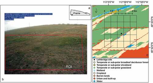
Figure 1. Location of the PhenoCam Lethbridge site in the Prairie Ecozone. (a) Field of view of the PhenoCam digital camera and the region of interest (red rectangle). (b) Land cover types of the surrounding area. (c) The surrounding area (marked by the 5 × 5 grid). Each grid square represents the footprint of a single 500-m MODIS pixel on the ground. The base map for the surrounding area is adapted from the 2010 Land Cover of Canada map (Canada center for mapping and earth observation under the open government license https://open.canada.ca/en/open-government-license-canada) complete with a map legend where only land cover types of the present spatial extent in the region of interest and surroundings are listed.

Additional products include daily and 3-day GCC time series. These data store the 90^th percentiles of all daytime GCC values for each day and 3-day window in which the impact of scene illumination changes on GCC was minimized (Richardson et al. 2017; Sonnentag et al. 2012). The daily GCC time series from 1 January 2012 to 31 December 2017 was used in conjunction with snow and data quality flags extracted from the PhenoCam Dataset V1.0 (Richardson et al. 2017). From this information set, near-surface remote sensing grassland phenology data were extracted for the validation of the grassland LSP metrics derived from MODIS VIs as described in Section 2.3.

2.2. MODIS daily VIs and multi-day composite VIs

The daily MODIS Nadir Bidirectional Reflectance Distribution Function (BRDF)-Adjusted Reflectance (NBAR) data were first downloaded using Global Subsets Tools (https://modis.ornl.gov/cgi-bin/MODIS/global/subset.pl) from the Oak Ridge National Laboratory Distributed Active Archive Center (ORNL DAAC) for a 5 × 5-pixel (approximately 2.5 × 2.5 km) area centered over the pixel where the PhenoCam Lethbridge site is located. The daily, 500-m MODIS MCD43A4 Version 6 NBAR (Schaaf and Wang 2015) were acquired to generate daily and multi-day MODIS VIs that correspond to the near-surface daily GCC time series. The NBAR data represent the nadir-view land surface reflectance at local solar noon of each pixel. The quality control (QC) of NBAR data was also included as well as the land cover data extracted from MODIS land cover maps (Friedl et al. 2010). While all 25 pixels were classified as grassland, the landscape homogeneity of each pixel was further examined using the 2010 land cover map of Canada (https://open.canada.ca/data/en/dataset/c688b87f-e85f-4842-b0e1-a8f79ebf1133) produced from Landsat 7 satellite images by the Canada Center for Mapping and Earth Observation (CCMEO). Based on the detailed land covers (Figure 1), pixels that were mostly covered with non-grass vegetation (mostly cropland) were excluded.

The QC data were also used to filter reflectance values that were not retrieved through BRDF inversions (QC = 255). The remaining NBAR data were then averaged daily to compute a time series of three types of MODIS VIs:

(2) $\mathrm{N}\mathrm{D}\mathrm{V}\mathrm{I}=\frac{{\rho }_{NIR}-{\rho }_{red}}{{\rho }_{NIR}+{\rho }_{red}}$(2)

(3) $\mathrm{E}\mathrm{V}\mathrm{I}2=2.5\ast \frac{{\rho }_{NIR}-{\rho }_{red}}{{\rho }_{NIR}+2.4\ast {\rho }_{red}+1}$(3)

(4) $\mathrm{G}\mathrm{C}\mathrm{C}\mathrm{p}\mathrm{p}=\frac{{\rho }_{green}}{{\rho }_{green}+{\rho }_{red}+{\rho }_{blue}}$(4)

where ${\rho }_{NIR}$, ${\rho }_{red}$, ${\rho }_{green}$, and ${\rho }_{blue}$ represent the MODIS NBAR in the near-infrared, red, green, and blue bands, respectively. NDVI and EVI2 were calculated due to their extensive use in the retrieval of LSP metrics (e.g. White et al. 2009; Cong et al. 2012; Moon et al. 2019; Zhang et al. 2018). Per-pixel GCC (GCCpp) was calculated to illustrate changes in pixel-level greenness as a MODIS VI for direct comparison to PhenoCam GCC as described in Cui et al. (2019).

The MODIS VIs calculated from NBAR data were used as the reference for the daily vegetation dynamics (VI_ref). To simulate the actual changes in the remotely sensed land surface reflectance, the daily cloud and snow records for the center MODIS pixel were gathered from MODIS MOD09GA Version 6 Terra Surface Reflectance Daily L2G Global (Vermote and Wolfe 2015). From these data, the daily VIs with explicit snow and cloud status attached to each value in the time series (VI₁) were generated. The MVC method was then applied to the VI₁ time series to simulate multi-day MODIS VIs resampled at 2-day time steps from 2 to 32 days (VI₂, VI₄, VI_6, VI₈, …, and VI₃₂). For each time window (2 ~ 32 days) across the VI₁ time series, the maximum cloud-free value or the maximum value (in the absence of cloud-free values in the window) was picked as the composite VI while its date and status of cloud and snow value were also recorded. Windows with no values (BRDF inversions failed for all NBAR data due to insufficient cloud-free observations) were left as gaps in the time series.

2.3. Modeling of the MODIS VIs and PhenoCam GCC time series

To estimate LSP metrics in prairie grasslands, the time series of daily MODIS VIs was smoothed and modeled to reveal the grassland growth trajectory, starting with the determination of the background VI values. Background VI is the bottom of the VI trajectory across the growing season, while the presence of snow would significantly alter the VI values and thus influence how background VI is identified (Huete et al. 2002; Zhang 2015). To ensure reliable and consistent snow detection, a MODIS VI was considered as snow-free only if all the following criteria were met: (1) the corresponding snow status flag absence of snow; (2) the corresponding daily mean temperature (Tdm) is higher than 5°C; (3) the corresponding MODIS NBAR normalized difference snow index (NDSI) is less than ‒0.2. The values of Tdm were calculated using the daily maximum and minimum temperature from a 1-km Daymet gridded weather dataset (Thornton et al. 2016), and 5°C is widely accepted as the temperature threshold for the vegetation photosynthetic activities out of winter periods (Zhang 2015; Zhang, Goldberg, and Yu 2012; Liu et al. 2017a). The NBAR NDSI values were calculated as

(5) $NDSI=\frac{{\rho }_{green}-{\rho }_{SWIR}}{{\rho }_{green}+{\rho }_{SWIR}}$(5)

where ${\rho }_{green}$ and ${\rho }_{SWIR}$ are the NBAR data in MODIS bands 4 (0.545–0.565 μm) and 6 (1.628–1.652 μm) to differentiate between snow cover and non-snow cover over MODIS pixels (Hall et al. 2002). Finally, the background VI for a given year was determined as the mean of the bottom 5^th percentile of clean values (i.e. cloud- and snow-free) during the active period (Tdm > 5°C) and the top 5^th percentile of clean values over the dormant season in a three-year period starting with the preceding year. Gaps and cloud-contaminated values along the time series were filled through linear interpolation using neighboring clean VIs (Ganguly et al. 2010).

The second step of the modeling process was validating the growing seasons during the time series. This step is challenging for grassland pixels because grasses are often mixed with forbs, shrubs, and other vegetation on the ground in the Prairie Ecozone (Li and Guo 2012). To accurately retrieve overall phenological changes, the temporal extent and magnitude of the VI time series that corresponded to the most significant vegetation dynamics were identified. The three-year period centered in the target year was first partitioned into multiple candidate growing seasons using all peaks (i.e. the local maximum VI) that are higher than the background VI by more than 35% of the period amplitude and both of the associated valleys (i.e. the local minimum VI between two neighboring peaks). Step two was the elimination of growing seasons that contains the peaks that are not the highest within 60 days. In the final step, the extent of the valid growing season(s) was bounded by the two lowest valleys associated with the highest peak of the target year. Seasonal dynamics over the valid growing season were retrieved by modeling the corresponding VI time series to the modified double logistic model (Elmore et al. 2012):

(6) $\mathrm{V}\mathrm{I}\left(t\right)=V{I}_{bg}+\left(V{I}_{amp}-f\ast t\right)\left(\frac{1}{1+e^{a\ast \left(b-t\right)}}-\frac{1}{1+e^{c\ast \left(d-t\right)}}\right)$(6)

where $t$ is the time in day of year (DOY), $\mathrm{V}\mathrm{I}\left(t\right)$ is the VI composite value at the day of $t$, $V{I}_{bg}$ and $V{I}_{amp}$ represent the background VI and amplitude of annual VI values, $b$ and $a$ represent the inflection point and the slope of the green-up period, respectively, $d$ and $c$ control the inflection point and the slope for the senescence period, and $f$ corresponds to the possible depression of vegetation growth during summer related to water stress (Elmore et al. 2012). The values of $a$, $b$, $c$, $d$, and $f$ were estimated using the Levenberg–Marquardt method and the modeled daily VI time series were obtained by using logistic models as a function of time at a daily step. The validation time series for MODIS VIs were generated from daily PhenoCam GCC in the same way.

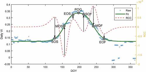
Seven phenological transition points in DOY across each growing season could be extracted from the modeled MODIS and PhenoCam daily time series using the rate of curvature change-based algorithm (Zhang et al. 2003). These metrics correspond to the onset of the start of spring (SOS), middle of spring (MOS), end of spring (EOS), start of fall (SOF), middle of fall (MOF), and end of greenness (EOF). Besides, the peak of the growing season (POG) representing the DOY when the modeled curve reaches the annual maximum was added as the transition from greenup to senescence to describe the complete phenological development of greenness measured from MODIS VIs. Figure 2 shows an example of using daily VI to estimate these metrics from the double logistic fit, according to the curvature change-based phenology retrieval algorithm described in Zhang et al. (2003).

Figure 2. Rate of curvature change (RCC)-based algorithm for the retrieval of phenological transition points.

2.4. Evaluating the quality of MODIS-based grassland phenology

The impact of temporal resolution on the quality of the estimated grassland phenology was investigated by examining the overall quality of modeled daily time series and the quality of each phenological metric. The changes in the average number of clean values used for growing season trajectory models were first surveyed as the temporal resolution changed. Two groups of coefficients of determination (r²) were then calculated to quantify the quality of the modeled daily time series. The first r² group was the relationship between the modeled and original values of all clean VIs in each simulated time series (r²_S) to reflect the fitness of the modeled time series at each temporal resolution. The second r² group was the relationship between the modeled values of all clean daily VI in each modeled daily time series and the corresponding values in the VI_ref time series (r²_R) to characterize the ability of VI time series with different temporal resolutions in predicting the daily variation in VI_ref. These values were computed for each year from 2001 to 2017 with mean values computed to reveal the overall quality of the modeled time series.

The quality of grassland phenological metrics was explored for the seven key phenological transitions based on the comparison between the MODIS-based onset of phenological metrics. Here the NDVI-based SOS (SOS_ndvi) was used as an example to briefly describe the procedures of the comparison. First, the average (means and medians) SOS_ndvi values from 2001 to 2017 were computed for each temporal resolution, with which the significance of the differences among average SOSs was assessed based on their normality. Specifically, a one-tailed t-test would be used when all groups of SOS_ndvi (one group for each temporal resolution) were normally distributed (the Kolmogorov–Smirnoff test was used for normality test). Otherwise, the non-parametric Wilcoxon signed-rank test would be applied to detect the significance of the difference between medians. Second, the magnitude of the interannual variation in SOSs related to changes in the temporal resolution was determined by calculating the standard deviation of each measure (SD) across all temporal resolutions, and then the difference between the SDs of simulated NDVIs-based SOS and those derived from the daily reference NDVI time series were assessed using an F-test. Finally, the trend in the temporal resolution-induced change in SOS_ndvi was estimated using simple linear regression where the SOS_ndvi derived from 1- to 32-day VIs and the temporal resolutions are the dependent and independent parameters, respectively. The slope of the linear relationship was computed and compared to zero which indicates no linear trend in the changes in SOS_ndvi and the temporal resolution of NDVI.

2.5. Assessing the accuracy of MODIS-based phenology

The MODIS-based phenological metrics were compared to corresponding onset dates derived from PhenoCam GCC time series to test uncertainty in the temporal resolution of satellite-based phenology estimates. Specifically, the daily MODIS VIs were examined against the multi-day MODIS VIs resampled at 8, 10, 14, and 16 days as they were used to generate the commonly used satellite VI products. The magnitudes of uncertainties for each phenological metric were quantified using mean bias errors (MBE) and mean absolute errors (MAE), which were computed as:

(7) $MBE=\frac{{\sum }_{i=1}^n\left(M_i-P_i\right)}{n}$(7)

(8) $MAE=\frac{{\sum }_{i=1}^n\left|M_i-P_i\right|}{n}$(8)

where $M_i$ and $P_i$ are the phenological metrics derived from time series of MODIS VIs and PhenoCam GCC from 2012 to 2017, respectively. The MBE and MAE for MODIS daily VI and multi-day VI composites were then compared to measure how they changed as the temporal resolution of MODIS VIs became coarser. The significance of the differences was assessed with either a one-tailed t-test or Wilcoxon signed-rank test depending on normality.

3. Results

3.1. Quality of modeled MODIS VI time series

A significant change was found in the number of clean values used to model the trajectories of grassland growing seasons as the temporal resolution of MODIS VIs changed from 1- to 32-day intervals (Figure 3(a)). In the daily time series, more than 100 clean VI values on average were found in each growing season from 2001 to 2017. The number of clean values in the MODIS VI time series decreases dramatically to less than 30 as the temporal resolution reached to 32 days. The fraction of clean values in each growing season increases from about 37% in a daily time series to near 100% in the 32-day VIs.

Figure 3. The overall quality of the modeled time series of MODIS VIs: the mean number of clean values in the growing seasons detected by MODIS VIs with different temporal resolutions (a); r²_S shows the mean coefficients of determination between modeled and original values of clean VIs in multi-day MODIS VIs (b); r²_R represents the mean coefficient of determination between modeled values of all clean daily VI in each modeled daily time series and the corresponding values in the daily reference time series (c). “R” are results obtained by using the daily reference MODIS VIs.

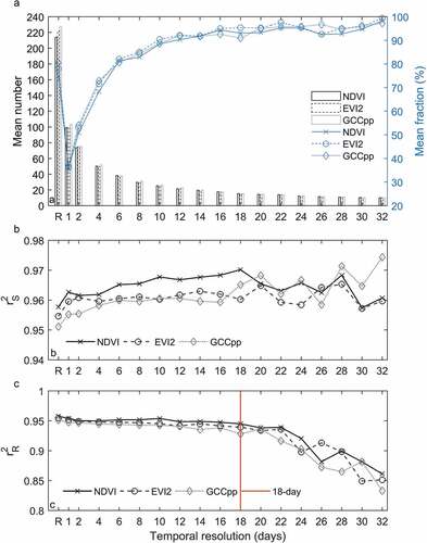
The double logistic model is reasonably effective in preserving the temporal variation in the input multi-day MODIS VIs, when the r² values change between 0.95 and 0.98 across temporal resolutions and types of MODIS VIs (Figure 3(b)). A descending trend was extracted in r²_R and a more rapid decline of r²_R was discovered as the temporal resolution becomes more coarse. For example, there is a sharp enhancement of the decline of r²_R in prior to and immediately after 18 days for three different types of MODIS VIs (Figure 3(c);Table 1).

Table 1. The rate of change in the quality of the modeled daily MODIS VIs time series relative to reference daily MODIS VIs time series as the temporal resolution increases from 1 to 32 days. Significance in rates of change are indicated by * (P < 0.05), ** (P < 0.01), or *** (P < 0.001).

MODIS VI	Rate of change (slope of linear fit)
	1- to 32-day	1- to 18-day	18- to 32-day
NDVI	−0.003***	−0.0003*	−0.006**
EVI2	−0.003***	−0.0006***	−0.007**
GCCpp	−0.003***	−0.0009***	−0.007**

3.2. Quality of MODIS-based grassland phenological metrics

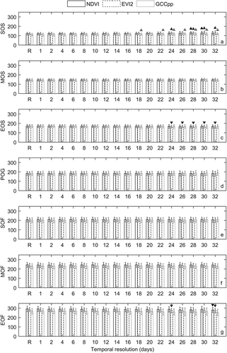
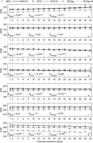
The comparison of phenological transition onsets shows that there is no significant difference between the mean MOS, POG, SOF, and MOF derived using the simulated daily and multi-day MODIS VIs and those estimated from the daily reference MODIS VIs (Figure 4(b), and d ~ f). In contrast, significantly delayed SOS estimates were obtained for the 28- and 30-day NDVI, 24-, 28-. 30-, and 32-day EVI2, and 18- and 22- to 32-day GCCpp (Figure 4(a)). However, earlier EOS was observed from EVI2 when the temporal resolution is coarser than 24 days (Figure 4(c)). Significant shifts to earlier onset were also apparent for EOF from 24- and 32-day NDVI and 32-day EVI2 (Figure 4(g)). But none of the significant difference was detected in the SDs, which indicates that the magnitudes of interannual variation in grassland phenological metrics estimated from simulated MODIS VIs are not statistically different from those retrieved from daily reference MODIS VIs.

Figure 4. Distribution of the mean onset of grassland phenological transitions derived from MODIS VIs with different temporal resolutions. All phenological transitions are normally distributed. Error bars are the standard deviation of each type of phenological transition. ▲ and ▼ above error bars locate mean onsets that are significantly higher and lower (P < 0.05) than those retrieved from the daily reference VI time series, respectively. “R” is the daily reference MODIS VI.

Linear regression analysis showed the different sensitivities of shifts in grassland phenology to the temporal resolution of MODIS VIs among phenological transitions and different types of MODIS VIs. A significantly late trend in SOS was revealed as the resampling frequency falls from daily to 32-day leading to SOS delayed by 8, 10, and 10 days when using NDVI, EVI2, and GCCpp, respectively (Figure 5(a)). The opposite shift toward early onset was observed for EOF which was advanced by 8, 7, and 11 days when the temporal resolution of NDVI, EVI2, and GCCpp changed from daily to the 32-day interval (Figure 5(g)). Therefore, the estimated duration of grassland greenness (the difference between the onset of EOF and SOS) will be shortened on average with MODIS VIs at coarser temporal resolution. Earlier trends with a smaller rate of change were found from EOS and SOF derived from NDVI and EVI2, which caused a shorter spring and fall estimated by NDVI and EVI2 and an extended summer because the advance of SOF was less than that of EOS (Figure 5(c,e)). Such changes in the length of summer and fall were even more substantial in GCCpp as the SOF tends to be later when the temporal resolution of GCCpp is coarser (Figure 5(e)). Different from other phenological transitions, MOS and MOF were not sensitive to temporal resolution change in MODIS VIs evidenced by the absence of significant shifts in the onset of these two phenological transitions (Figure 5(b,f)).

Figure 5. Linear trends in the mean onset of grassland phenological transitions (DOY) as a function of MODIS VI temporal resolution. S_NDVI, S_EVI2, and S_GCCpp are the slopes of the linear fits of the phenological transitions derived using MODIS NDVIs, EVI2s, and GCCpps, respectively. Significant differences are indicated by *, **, and *** for P < 0.05, 0.01, and 0.001, respectively.

3.3. Accuracy of MODIS-based grassland phenology

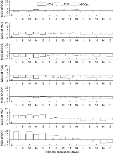
Compared to the onset of grassland phenological transitions measured from daily PhenoCam GCC, the daily NDVI-based phenological transitions were earlier during the greenup phase (POG included) and later during senescence. MBE ranged from ‒3.5 days for EOS to 21.5 days for EOF (Figure 6). A similar pattern was observed for the MBE of phenological transitions derived from daily EVI2 with relatively reduced magnitudes (except for POG). The negative MBEs of all GCCpp-based phenological metrics indicate a consistently earlier onset of grassland phenological development measured from MODIS GCCpp. When using multi-day MODIS VIs, less MBE was retrieved at various magnitudes for different phenological transitions and MODIS VI types (except for EOS), e.g. the MBE of EOF changed from 10.8 to 3.5 days using 16-day EVI2 (Figure 6(g)) and MBE of SOS derived from GCCpp decreased from ‒6.5 to ‒1 days when the temporal resolutions reached the 16-day interval (Figure 6(a)). Besides, more evident advance or delay of phenological transitions onsets such as EOS and POG were calculated by using 14-day VIs (Figure 6(c,d)). However, none of these variations in MBEs were statistically significant.

Figure 6. The mean bias errors (MBE) of MODIS-based phenological metrics.

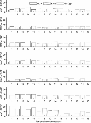
The MAEs of daily NDVI-based grassland phenological metrics were less than 10 days across the growing seasons except for EOF. A similar temporal pattern was observed from the MAE of grassland phenological metrics derived from EVI2 and GCCpp (Figure 7). Daily NDVI-based MAE of POG and SOF were smaller than those derived from daily EVI2 and GCCpp, and it seemed better to use daily EVI2 and GCCpp for the remaining phenological transitions. Like MBE, variations of MAEs in grassland phenological metrics were discovered for multi-day MODIS VIs, including improved accuracy of SOS by using 16-day GCCpp (Figure 7(a)) and reduced accuracy of EOS estimated from 14-day VIs (Figure 7(c)). All variations in MAEs of grassland phenological transitions onsets were statistically insignificant.

Figure 7. The mean absolute errors (MAE) of MODIS-based phenological metrics.

4. Discussion

In areas with no in situ phenology observations, it is difficult to evaluate the LSP retrieved from remote sensing data. The approach developed in this study involves the near-surface PhenoCam phenology observations as the validation dataset and performs a quantitative analysis of the impact of temporal resolution of satellite VIs on the quality and accuracy of the retrieved LSP of prairie grasslands. As a note of caution for further research, there is only one PhenoCam grassland site in the Prairie Ecozone. Therefore, it is still hard to fully understand the influence of characteristics of remote sensing data on the estimated LSP of grasslands.

Multi-angle reflectance products (Alexandridis, Gitas, and Silleos 2008) or 16-day NBAR data (Zhang, Friedl, and Schaaf 2009) have been previously used to assess the impact of temporal resolution of MODIS data on vegetation phenology monitoring. In this study, the daily MODIS NBAR data were used to provide a more accurate approximation of detailed temporal vegetation dynamics as the data source (Ju et al. 2010). The multi-day MODIS composite VIs were then simulated using actual daily cloud and snow status during the acquisition of MODIS observations. Like most previous studies, the MVC method was employed to select the best cloud-free composite VI, which proves to be effective in picking clean values (Figure 3(a)). Moreover, the temporal resolutions used in this study have a relatively wide range (1–32 days) and small time step (2 days) than used in previous studies (Kross et al. 2011; Zhang, Friedl, and Schaaf 2009). Therefore, this study not only covers the temporal resolution of most commonly used composite VIs but also explored the capability of coarse-temporal resolution satellite data such as 10-day SPOT VGT, 15-day GIMMS NDVI3g, and 16-day Landsat surface reflectance in the measurement of grassland phenology when the observations are contaminated by clouds.

MODIS VIs in this study were modeled for grassland phenology estimation with more accurate detection of background VI. The value of background VI is critical for accurate land surface phenology estimation (Moon et al. 2019). Although various algorithms were developed to find the background VI, they all rely on the accurate detection of snow along the time series (Zhang et al. 2003; Zhang 2015; Zhang et al. 2018; Moon et al. 2019; Ganguly et al. 2010). By applying an integrated screening approach, the effect of snow during the winter was minimized. Furthermore, neither the closest snow-free values as in Ganguly et al. (2010) nor an empirical value such as 0.2 (Alexandridis, Gitas, and Silleos 2008) or 0.1 or 0.15 (Hird and McDermid 2009) was used as the background VI to fill the gaps caused by snow for two principal reasons: extreme values may still exist over the winter period or around the start of spring, which may become more severe in a high-temporal-resolution time series (Figure 2), and empirical values are often region-specific. Instead, a relatively unbiased background VI that is subject to nothing but the statistical distribution of the VI was computed similar to Zhang (2015).

The impact of the temporal resolution of MODIS VIs was evaluated on both phenological transitions and the whole growing season trajectory. It is not surprising to find that, as shown in Figure 3(c) and previous research (Wang et al. 2017; McKellip et al. 2005; Narasimhan and Stow 2010), higher-temporal-resolution VIs are favorable to reflect high-frequency (e.g. daily) or sharp vegetation dynamics such as phenological transitions because they contain more high-quality, clean values across entire growing seasons. Similar results were obtained by Kross et al. (2011) in Canadian broadleaf deciduous forests. Statistically equal mean and interannual variation in phenological metrics derived from MODIS VIs were revealed when the temporal resolution was finer than a 18-day time interval. These findings indicate wide ranges of favorable temporal resolution of satellite VIs to extract trends in phenology changes for different ecosystems. One possible reason for this wide range is that a high density of clean (cloud- and snow-free) observations in the daily time series (Figure 3(a)) enables high-quality VIs near the phenological metric onset resulting in accurate timing estimates (Cao et al. 2015; Zhang 2015; Zhang et al. 2018). Another possible reason may be related to the use of logistic models (Equation (6)(6) $\mathrm{V}\mathrm{I}\left(t\right)=V{I}_{bg}+\left(V{I}_{amp}-f\ast t\right)\left(\frac{1}{1+e^{a\ast \left(b-t\right)}}-\frac{1}{1+e^{c\ast \left(d-t\right)}}\right)$(6) )(6) $\mathrm{V}\mathrm{I}\left(t\right)=V{I}_{bg}+\left(V{I}_{amp}-f\ast t\right)\left(\frac{1}{1+e^{a\ast \left(b-t\right)}}-\frac{1}{1+e^{c\ast \left(d-t\right)}}\right)$(6) in the simulation of the ideal annual trajectories of MODIS VIs (Figure 2). These results correspond to the conclusion from Zhang, Friedl, and Schaaf (2009) and confirm that the shifts in phenological metrics identified in the logistic model fit of multi-day VIs are not sensitive to either the noise or limited missing values in source daily data. Studies also suggest logistic models, including single (White, Pontius, and Schaberg 2014; Moon et al. 2019) and double logistic models (Atkinson et al. 2012; Hird and McDermid 2009) are superior to other fitting methods to suppress the influence of noise and missing values and predict accurate phenological transitions, as shown by the r²_S consistently higher than 0.95 in Figure 3(b). Therefore, the similar quality among the grassland phenology derived with different temporal resolutions may be partially ascribed to the use of the logistic model. However, a more significant decrease in r²_R than r²_S as the temporal resolution of MODIS VIs increases was observed. This may be caused by the too limited good-quality observations in the MODIS VIs resampled at coarse temporal intervals, which has extensively restricted the application of logistic models in predicting the details of temporal dynamics of MODIS daily reference VIs.

Finally, different MBE and MAE of phenological metrics were found as the temporal resolution of MODIS VIs changed (Figures 6 and 7). Consistent with Richardson et al. (2018b) and Zhang et al. (2018), grassland phenological metrics during greenup and senescence measured from near-surface PhenoCam data are generally delayed and advanced, respectively, compared to those estimated from MODIS data. This reflects different sensitivity of satellite VIs and PhenoCam color indices to the seasonal dynamics of plant canopy greenness in different growing phases. In addition, the spatial heterogeneity of our study area may also contribute to errors in MODIS-based grassland phenology as suggested in Hufkens et al. (2012) and Liu et al. (2017b). Shifts in phenological transition onsets from daily to 16-day temporal resolution are mainly attributed to the trend in grassland phenology change as a function of the temporal resolution of MODIS VIs (Figure 5). Similar trends were observed by Kandasamy and Fernandes (2015) for grassland SOS and EOF concerning the number of cloud-free VIs across growing seasons. MVC-based composite methods may also contribute to those trends as they tend to pick the value in the latter half of the compositing period before POG and the value in the former half after POG (Narasimhan and Stow 2010); therefore, the onset of SOS and EOF may move toward the peak of growing season as the resampling frequency shortens.

5. Conclusions

This study investigated the impact of temporal resolution of MODIS VIs on the retrieved phenology of grassland in the Prairie Ecozone using daily and multi-day composite NDVI, EVI2, and GCCpp calculated from the MODIS NBAR data. The results show that the quality and accuracy of key phenological transitions are not sensitive to changes in the temporal resolution of MODIS VIs when using MVC compositing methods and a logistic model-based fitting approach. For several temporal resolutions coarser than 18 days, significant differences were observed between the phenological metrics derived from MODIS multi-day and daily reference VIs. These findings were further confirmed by the evaluation of MODIS-based grassland phenology relative to those derived from near-surface PhenoCam GCC, which shows there is no significant difference in MBE and MAE in the onset of grassland phenological metrics retrieved from daily, 8-day, 10-day, 14-day, and 16-day MODIS VIs. Also, the ability of MODIS composite VIs to predict the detailed dynamics in daily reference VI was found to be significantly influenced by a change in the temporal resolution. A variety of trends in the shift of grassland phenological transition onsets were also extracted as a function of the temporal resolution of MODIS VIs. In general, MODIS VIs with temporal resolution finer than 18 days are favorable to estimate individual phenological transitions and the detailed temporal dynamics in the greenness measured from MODIS VIs.

This study presents a PhenoCam-involved approach to the evaluation of the impact of temporal resolution of satellite VIs on the quality and accuracy of the estimated phenological metrics of areas with no in situ phenology observations. Due to the limited validation dataset, this study was restricted in the prairie grassland near Lethbridge. In the future, more PhenoCam sites or a larger study area with available validation datasets should be included to verify the results obtained in this study and to further understand the uncertainties of satellite-based grassland phenology in relation to the temporal resolution of input satellite VIs. Our results also confirm that the use of logistic model-based fitting and obtaining clean (snow- and cloud-free), high-quality observations from the satellite may have played important roles in capturing accurate phenological developments in vegetation growth. These factors could be further verified by implementing phenology extraction from satellite data with a different fitting approach, such as splines (Richardson et al. 2018a; Moon et al. 2019) or polynomial functions (Narasimhan and Stow 2010). Besides, in regions where it is relatively hard to acquire clean remotely sensed observations, such as alpine or arctic grasslands, improving the certainty in the estimation of vegetation phenology related to the temporal resolution of satellite data will also be a significant advance.

Acknowledgements

The authors thank the Oak Ridge National Laboratory Distributed Active Archive Center (ORNL DAAC) for access to the PhenoCam Dataset V1.0 and the Daymet daily weather data and NASA Earth Observing System Data and Information System Land Processes Distributed Active Archive Center (LP DAAC) for access to the MODIS NBAR data.

The authors thank the Northeastern States Research Cooperative, NSF’s Macrosystems Biology program [awards EF-1065029 and EF-1702697], DOE’s Regional and Global Climate Modeling program [award DE-SC0016011], the US National Park Service Inventory and Monitoring Program and the USA National Phenology Network [grant number G10AP00129 from the United States Geological Survey], and the USA National Phenology Network and the North Central Climate Science Center [cooperative agreement number G16AC00224 from the United States Geological Survey] for their support of the development of PhenoCam. Research at the Lethbridge Grassland Ecosystem site is supported by NSERC [grant RGPIN-2014-05882] to L.B. Flanagan.

Disclosure statement

No potential conflict of interest was reported by the authors.

Additional information

Funding

This study is supported by the Natural Sciences and Engineering Research Council of Canada (NSERC) Discovery Grant: Integrating measures of grassland function using Remote Sensing and the NSERC Discovery Grant: Hydrological thresholds in depression storage and contributing area for low-relief landscapes.

References

- Ahl, D. E., S. T. Gower, S. N. Burrows, N. V. Shabanov, R. B. Myneni, and Y. Knyazikhin. 2006. “Monitoring Spring Canopy Phenology of a Deciduous Broadleaf Forest Using MODIS.” Remote Sensing of Environment 104 (1): 88–95. doi:10.1016/j.rse.2006.05.003.
- Alexandridis, T. K., I. Z. Gitas, and N. G. Silleos. 2008. “An Estimation of the Optimum Temporal Resolution for Monitoring Vegetation Condition on a Nationwide Scale Using MODIS/Terra Data.” International Journal of Remote Sensing 29 (12): 3589–3607. doi:10.1080/01431160701564618.
- Atkinson, P. M., C. Jeganathan, J. Dash, and C. Atzberger. 2012. “Inter-comparison of Four Models for Smoothing Satellite Sensor Time-series Data to Estimate Vegetation Phenology.” Remote Sensing of Environment 123: 400–417. doi:10.1016/j.rse.2012.04.001.
- Bradley, B. A., R. W. Jacob, J. F. Hermance, and J. F. Mustard. 2007. “A Curve Fitting Procedure to Derive Inter-annual Phenologies from Time Series of Noisy Satellite NDVI Data.” Remote Sensing of Environment 106 (2): 137–145. doi:10.1016/j.rse.2006.08.002.
- Burke, I. C., C. M. Yonker, W. J. Parton, C. V. Cole, D. Schimel, and K. Flach. 1989. “Texture, Climate, and Cultivation Effects on Soil Organic Matter Content in US Grassland Soils.” Soil Science Society of America Journal 53 (3): 800–805. doi:10.2136/sssaj1989.03615995005300030029x.
- Cao, R. Y., J. Chen, M. G. Shen, and Y. H. Tang. 2015. “An Improved Logistic Method for Detecting Spring Vegetation Phenology in Grasslands from MODIS EVI Time-series Data.” Agricultural and Forest Meteorology 200: 9–20. doi:10.1016/j.agrformet.2014.09.009.
- Cong, N., S. Piao, A. Chen, X. Wang, X. Lin, S. Chen, S. Han, G. Zhou, and X. Zhang. 2012. “Spring Vegetation Green-up Date in China Inferred from SPOT NDVI Data: A Multiple Model Analysis.” Agricultural and Forest Meteorology 165: 104–113. doi:10.1016/j.agrformet.2012.06.009.
- Cui, T., L. Martz, E. G. Lamb, L. Zhao, and X. Guo. 2019. “Comparison of Grassland Phenology Derived from MODIS Satellite and PhenoCam Near-Surface Remote Sensing in North America.” Canadian Journal of Remote Sensing 45 (5): 707–722. doi:10.1080/07038992.2019.1674643.
- Cui, T., L. Martz, and X. Guo. 2017. “Grassland Phenology Response to Drought in the Canadian Prairies.” Remote Sensing 9 (12): 1258. doi:10.3390/rs9121258.
- Dye, D. G., B. R. Middleton, J. M. Vogel, Z. Wu, and M. Velasco. 2016. “Exploiting Differential Vegetation Phenology for Satellite-Based Mapping of Semiarid Grass Vegetation in the Southwestern United States and Northern Mexico.” Remote Sensing 8 (11): 889. Unsp. doi:10.3390/Rs8110889.
- Eidenshink, J. C. 1992. “The 1990 Conterminous United-States Avhrr Data Set.” Photogrammetric Engineering and Remote Sensing 58 (6): 809–813.
- Elmore, A. J., S. M. Guinn, B. J. Minsley, and A. D. Richardson. 2012. “Landscape Controls on the Timing of Spring, Autumn, and Growing Season Length in mid‐Atlantic Forests.” Global Change Biology 18 (2): 656–674. doi:10.1111/j.1365-2486.2011.02521.x.
- Friedl, M. A., D. Sulla-Menashe, B. Tan, A. Schneider, N. Ramankutty, A. Sibley, and X. Huang. 2010. “MODIS Collection 5 Global Land Cover: Algorithm Refinements and Characterization of New Datasets.” Remote Sensing of Environment 114 (1): 168–182. doi:10.1016/j.rse.2009.08.016.
- Ganguly, S., M. A. Friedl, B. Tan, X. Zhang, and M. Verma. 2010. “Land Surface Phenology from MODIS: Characterization of the Collection 5 Global Land Cover Dynamics Product.” Remote Sensing of Environment 114 (8): 1805–1816. doi:10.1016/j.rse.2010.04.005.
- Gillespie, A. R., A. B. Kahle, and R. E. Walker. 1987. “Color Enhancement of Highly Correlated Images .2. Channel Ratio and Chromaticity Transformation Techniques.” Remote Sensing of Environment 22 (3): 343–365. doi:10.1016/0034-4257(87)90088-5.
- Hall, D. K., G. A. Riggs, V. V. Salomonson, N. E. DiGirolamo, and K. J. Bayr. 2002. “MODIS Snow-cover Products.” Remote Sensing of Environment 83 (1–2): 181–194. Pii S0034-4257(02)00095-0. doi:10.1016/S0034-4257(02)00095-0.
- Hird, J. N., and G. J. McDermid. 2009. “Noise Reduction of NDVI Time Series: An Empirical Comparison of Selected Techniques.” Remote Sensing of Environment 113 (1): 248–258. doi:10.1016/j.rse.2008.09.003.
- Holben, B. N. 1986. “Characteristics of Maximum-value Composite Images from Temporal AVHRR Data.” International Journal of Remote Sensing 7 (11): 1417–1434. doi:10.1080/01431168608948945.
- Huete, A., K. Didan, T. Miura, E. P. Rodriguez, X. Gao, and L. G. Ferreira. 2002. “Overview of the Radiometric and Biophysical Performance of the MODIS Vegetation Indices.” Remote Sensing of Environment 83 (1): 195–213. doi:10.1016/S0034-4257(02)00096-2.
- Hufkens, K., M. Friedl, O. Sonnentag, B. H. Braswell, T. Milliman, and A. D. Richardson. 2012. “Linking Near-surface and Satellite Remote Sensing Measurements of Deciduous Broadleaf Forest Phenology.” Remote Sensing of Environment 117: 307–321. doi:10.1016/j.rse.2011.10.006.
- Jiang, Z. Y., A. R. Huete, K. Didan, and T. Miura. 2008. “Development of a Two-band Enhanced Vegetation Index without a Blue Band.” Remote Sensing of Environment 112 (10): 3833–3845. doi:10.1016/j.rse.2008.06.006.
- Ju, J. C., D. P. Roy, Y. M. Shuai, and C. Schaaf. 2010. “Development of an Approach for Generation of Temporally Complete Daily Nadir MODIS Reflectance Time Series.” Remote Sensing of Environment 114 (1): 1–20. doi:10.1016/j.rse.2009.05.022.
- Kandasamy, S., and R. Fernandes. 2015. “An Approach for Evaluating the Impact of Gaps and Measurement Errors on Satellite Land Surface Phenology Algorithms: Application to 20 Year NOAA AVHRR Data over Canada.” Remote Sensing of Environment 164: 114–129. doi:10.1016/j.rse.2015.04.014.
- Keenan, T. F., B. Darby, E. Felts, O. Sonnentag, M. A. Friedl, K. Hufkens, J. O’Keefe, et al. 2014. “Tracking Forest Phenology and Seasonal Physiology Using Digital Repeat Photography: A Critical Assessment.” Ecological Applications 24 (6): 1478–1489. doi:10.1890/13-0652.1.
- Kross, A., R. Fernandes, J. Seaquist, and E. Beaubien. 2011. “The Effect of the Temporal Resolution of NDVI Data on Season Onset Dates and Trends across Canadian Broadleaf Forests.” Remote Sensing of Environment 115 (6): 1564–1575. doi:10.1016/j.rse.2011.02.015.
- Lesica, P., and P. Kittelson. 2010. “Precipitation and Temperature are Associated with Advanced Flowering Phenology in a Semi-arid Grassland.” Journal of Arid Environments 74 (9): 1013–1017. doi:10.1016/j.jaridenv.2010.02.002.
- Li, Z., and X. Guo. 2012. “Detecting Climate Effects on Vegetation in Northern Mixed Prairie Using NOAA AVHRR 1-km Time-series NDVI Data.” Remote Sensing 4 (1): 120–134. doi:10.3390/rs4010120.
- Liu, L., X. Zhang, Y. Yu, and W. Guo. 2017a. “Real-time and Short-term Predictions of Spring Phenology in North America from VIIRS Data.” Remote Sensing of Environment 194 (Supplement C): 89–99. doi:10.1016/j.rse.2017.03.009.
- Liu, Y., M. J. Hill, X. Zhang, Z. Wang, A. D. Richardson, K. Hufkens, G. Filippa, D. D. Baldocchi, S. Ma, and J. Verfaillie. 2017b. “Using Data from Landsat, MODIS, VIIRS and PhenoCams to Monitor the Phenology of California Oak/grass Savanna and Open Grassland across Spatial Scales.” Agricultural and Forest Meteorology 237: 311–325. doi:10.1016/j.agrformet.2017.02.026.
- McKellip, R., R. E. Ryan, S. Blonski, and D. Prados. 2005. “Crop Surveillance Demonstration Using a Near-daily MODIS Derived Vegetation Index Time Series.”
- Moon, M., X. Zhang, G. M. Henebry, L. Liu, J. M. Gray, E. K. Melaas, and M. A. Friedl. 2019. “Long-term Continuity in Land Surface Phenology Measurements: A Comparative Assessment of the MODIS Land Cover Dynamics and VIIRS Land Surface Phenology Products.” Remote Sensing of Environment 226: 74–92. doi:10.1016/j.rse.2019.03.034.
- Narasimhan, R., and D. Stow. 2010. “Daily MODIS Products for Analyzing Early Season Vegetation Dynamics across the North Slope of Alaska.” Remote Sensing of Environment 114 (6): 1251–1262. doi:10.1016/j.rse.2010.01.017.
- Pinzon, J. E., and C. J. Tucker. 2014. “A Non-Stationary 1981-2012 AVHRR NDVI3g Time Series.” Remote Sensing 6 (8): 6929–6960. doi:10.3390/rs6086929.
- Pouliot, D., R. Latifovic, R. Fernandes, and I. Olthof. 2011. “Evaluation of Compositing Period and AVHRR and MERIS Combination for Improvement of Spring Phenology Detection in Deciduous Forests.” Remote Sensing of Environment 115 (1): 158–166. doi:10.1016/j.rse.2010.08.014.
- Reed, B. C. 2006. “Trend Analysis of Time-series Phenology of North America Derived from Satellite Data.” GIScience & Remote Sensing 43 (1): 24–38. doi:10.2747/1548-1603.43.1.24.
- Reed, B. C., J. F. Brown, D. Vanderzee, T. R. Loveland, J. W. Merchant, and D. O. Ohlen. 1994. “Measuring Phenological Variability from Satellite Imagery.” Journal of Vegetation Science 5 (5): 703–714. doi:10.2307/3235884.
- Richardson, A. D., K. Hufkens, T. Milliman, D. M. Aubrecht, M. Chen, J. M. Gray, M. R. Johnston, et al. 2017. “PhenoCam Dataset V1.0: Vegetation Phenology from Digital Camera Imagery, 2000–2015.” ORNL DAAC, Oak Ridge, Tennessee, USA. https://doi.org/10.3334/ORNLDAAC/1511
- Richardson, A. D., K. Hufkens, T. Milliman, D. M. Aubrecht, M. Chen, J. M. Gray, M. R. Johnston, T. F. Keenan, S. T. Klosterman, and M. Kosmala. 2018a. “Tracking Vegetation Phenology across Diverse North American Biomes Using PhenoCam Imagery.” Scientific Data 5: 180028. doi:10.1038/sdata.2018.28.
- Richardson, A. D., K. Hufkens, T. Milliman, and S. Frolking. 2018b. “Intercomparison of Phenological Transition Dates Derived from the PhenoCam Dataset V1.0 And MODIS Satellite Remote Sensing.” Scientific Reports 8 (1): 5679. doi:10.1038/s41598-018-23804-6.
- Richardson, A. D., T. F. Keenan, M. Migliavacca, Y. Ryu, O. Sonnentag, and M. Toomey. 2013. “Climate Change, Phenology, and Phenological Control of Vegetation Feedbacks to the Climate System.” Agricultural and Forest Meteorology 169: 156–173. doi:10.1016/j.agrformet.2012.09.012.
- Schaaf, C., and Z. Wang 2015. “MCD43A4 MODIS/Terra.þAqua BRDF/Albedo Nadir BRDF Adjusted Ref Daily L3 Global - 500m V006” (dataset). NASA EOSDIS Land Processes DAAC. Accessed May 14, 2019. https://doi.10.5067/MODIS/MCD43A4.006
- Sonnentag, O., K. Hufkens, C. Teshera-Sterne, A. M. Young, M. Friedl, B. H. Braswell, T. Milliman, J. O’Keefe, and A. D. Richardson. 2012. “Digital Repeat Photography for Phenological Research in Forest Ecosystems.” Agricultural and Forest Meteorology 152: 159–177. doi:10.1016/j.agrformet.2011.09.009.
- Thornton, P. E., M. M. Thornton, B. W. Mayer, Y. Wei, R. Devarakonda, R. S. Vose, and R. B. Cook. 2016. “Daymet: Daily Surface Weather Data on a 1-km Grid for North America, Version 3.” ORNL DAAC, Oak Ridge, Tennessee, USA. https://doi.org/10.3334/ORNLDAAC/1328
- Toomey, M., M. A. Friedl, S. Frolking, K. Hufkens, S. Klosterman, O. Sonnentag, D. D. Baldocchi, et al. 2015. “Greenness Indices from Digital Cameras Predict the Timing and Seasonal Dynamics of Canopy-scale Photosynthesis.” Ecological Applications 25 (1): 99–115. doi:10.1890/14-0005.1.
- Tucker, C. J. 1979. “Red and Photographic Infrared Linear Combinations for Monitoring Vegetation.” Remote Sensing of Environment 8 (2): 127–150. doi:10.1016/0034-4257(79)90013-0.
- Vermote, E., and R. Wolfe 2015. “MOD09GA MODIS/Terra Surface Reflectance Daily L2G Global 1kmand500m SIN Grid V006” (dataset). NASA EOSDIS Land Processes DAAC. Accessed May, 14, 2019. https://doi 10.5067/MODIS/MOD09GA.006
- Wang, W., and J. Fang. 2009. “Soil Respiration and Human Effects on Global Grasslands.” Global and Planetary Change 67 (1–2): 20–28. doi:10.1016/j.gloplacha.2008.12.011.
- Wang, Z. S., C. B. Schaaf, Q. S. Sun, J. Kim, A. M. Erb, F. Gao, M. O. Roman, et al. 2017. “Monitoring Land Surface Albedo and Vegetation Dynamics Using High Spatial and Temporal Resolution Synthetic Time Series from Landsat and the MODIS BRDF/NBAR/albedo Product.” International Journal of Applied Earth Observation and Geoinformation 59: 104–117. doi:10.1016/j.jag.2017.03.008.
- White, K., J. Pontius, and P. Schaberg. 2014. “Remote Sensing of Spring Phenology in Northeastern Forests: A Comparison of Methods, Field Metrics and Sources of Uncertainty.” Remote Sensing of Environment 148: 97–107. doi:10.1016/j.rse.2014.03.017.
- White, M. A., K. M. de Beurs, K. Didan, D. W. Inouye, A. D. Richardson, O. P. Jensen, J. O’Keefe, et al. 2009. “Intercomparison, Interpretation, and Assessment of Spring Phenology in North America Estimated from Remote Sensing for 1982–2006.” Global Change Biology 15 (10): 2335–2359. doi:10.1111/j.1365-2486.2009.01910.x.
- Xin, Q. C., M. Broich, P. Zhu, and P. Gong. 2015. “Modeling Grassland Spring Onset across the Western United States Using Climate Variables and MODIS-derived Phenology Metrics.” Remote Sensing of Environment 161: 63–77. doi:10.1016/j.rse.2015.02.003.
- Yuan, F., C. Wang, and M. Mitchell. 2014. “Spatial Patterns of Land Surface Phenology Relative to Monthly Climate Variations: US Great Plains.” GIScience & Remote Sensing 51 (1): 30–50. doi:10.1080/15481603.2014.883210.
- Zhang, X. 2015. “Reconstruction of a Complete Global Time Series of Daily Vegetation Index Trajectory from Long-term AVHRR Data.” Remote Sensing of Environment 156 (Supplement C): 457–472. doi:10.1016/j.rse.2014.10.012.
- Zhang, X., M. A. Friedl, and C. B. Schaaf. 2006. “Global Vegetation Phenology from Moderate Resolution Imaging Spectroradiometer (MODIS): Evaluation of Global Patterns and Comparison with in Situ Measurements.” Journal of Geophysical Research-Biogeosciences 111: G4. doi:10.1029/2006jg000217.
- Zhang, X., M. A. Friedl, and C. B. Schaaf. 2009. “Sensitivity of Vegetation Phenology Detection to the Temporal Resolution of Satellite Data.” International Journal of Remote Sensing 30 (8): 2061–2074. doi:10.1080/01431160802549237.
- Zhang, X., M. A. Friedl, C. B. Schaaf, A. H. Strahler, J. C. F. Hodges, F. Gao, B. C. Reed, and A. Huete. 2003. “Monitoring Vegetation Phenology Using MODIS.” Remote Sensing of Environment 84 (3): 471–475. doi:10.1016/S0034-4257(02)00135-9.
- Zhang, X., M. D. Goldberg, and Y. Yu. 2012. “Prototype for Monitoring and Forecasting Fall Foliage Coloration in Real Time from Satellite Data.” Agricultural and Forest Meteorology 158–159 (Supplement C): 21–29. doi:10.1016/j.agrformet.2012.01.013.
- Zhang, X., S. Jayavelu, L. Liu, M. A. Friedl, G. M. Henebry, Y. Liu, C. B. Schaaf, A. D. Richardson, and J. Gray. 2018. “Evaluation of Land Surface Phenology from VIIRS Data Using Time Series of PhenoCam Imagery.” Agricultural and Forest Meteorology 256–257: 137–149. doi:10.1016/j.agrformet.2018.03.003.