Biome-level relationships between vegetation indices and climate variables using time-series analysis of remotely-sensed data

ABSTRACT

Climatic factors such as rainfall and temperature play a vital role in the growth characteristics of vegetation. While the relationship between climate and vegetation growth can be accurately predicted in instances where vegetation is homogenous, this becomes complex to determine in heterogeneous vegetation environments. The aim of this paper was to study the relationship between remotely-sensed monthly vegetation indices (i.e. Normalized Difference Vegetation Index and Enhanced Vegetation Index) and climatic variables (temperature and precipitation) using time-series analysis at the biome-level. Specifically, the autoregressive distributed lag model (ARDL1 and ARDL2, corresponding respectively to one month and two month lags) and the Koyck-transformed distributed lag model were used to build regression models. All three models estimated NDVI and EVI fairly accurately in all biomes (Relative Root-Mean-Squared-Error (RMSE): 12.0–26.4%). Biomes characterized by relative homogeneity (Grassland, Savanna, Indian Ocean Coastal Belt and Forest Biomes) achieved the most accurate estimates due to the dominance of a few species. Comparisons of lag size (one month compared to two months) generally showed similarities (Akaike Information Criterion (AIC), Bayesian Information Criterion (BIC) and log-likelihood) with quite high comparability in certain biomes – this indicates the utility of the ARDL1 and ARDL2 model, depending on the availability of appropriate data. These findings demonstrate the variation in estimation linked to the biome, and thus the validity of biome-level correlation of climatic data and vegetation indices.

KEYWORDS:

• Enhanced Vegetation Index
• normalized Difference Vegetation Index
• MODIS
• time-series analysis
• distributed lag model
• temperature
• precipitation

Introduction

Vegetation plays a critical role in regulating climatic dynamics, in hydrological processes and serving as an interface for energy flux between the atmosphere and terrestrial systems (McPherson 2007; Liu and Ren 2012; Musau et al. 2016). Vegetation dynamics are also influenced by various climatic and landscape characteristics such as topography and soil (Chamaille‐Jammes, Fritz, and Murindagomo 2006; Kim 2013; Whetton et al. 2017). Therefore, the process of monitoring vegetation dynamics, as well as the predicting of future scenarios, benefits greatly by factoring in growth-influencing aspects (Scanlon et al. 2002; Wang, Rich, and Price 2003). Considering the spatial nature of both vegetation distribution and climate variation, efficient data collection and interpretation techniques for monitoring should be sought. Remote sensing is an efficient option and has been used for a plethora of applications including plant phenology monitoring (e.g. Zhang et al. 2005; Yuan, Wang, and Mitchell 2014; Pan et al. 2015; Ding et al. 2016), monitoring grassland dynamics (Li et al. 2013), monitoring ecosystem dynamics (Zewdie, Csaplovics, and Inostroza 2017), hydrological modeling (Murray, Watson, and Prentice 2012; Birtwistle et al. 2016), landscape degradation assessment (Holm, Cridland, and Roderick 2003; Eckert et al. 2015; Schultz et al. 2016), plant disease mapping (Eklundh, Johansson, and Solberg 2009) and plant invasion monitoring (Bradley and Mustard 2006). Efficient monitoring is a pressing matter in the face of both climate change and environmental degradation, which require timely mitigation (Holm, Cridland, and Roderick 2003; Balaghi et al. 2008; Omuto et al. 2010; Li et al. 2013; Chen et al. 2015; Jiang et al. 2017; Pang, Wang, and Yang 2017; Ren, Chen, and An 2017; Zewdie, Csaplovics, and Inostroza 2017; Zheng et al. 2018). Remote sensing and time-series analysis provide useful information in this regard by correlating vegetation dynamics with climatic variables (e.g. Chamaille‐Jammes, Fritz, and Murindagomo 2006; Chu, Lu, and Zhang 2007; Xian, Homer, and Aldridge 2012; Boschetti et al. 2013; Yuan, Wang, and Mitchell 2014; Fu and Burgher 2015; Barbosa and Lakshmi Kumar 2016; Ding et al. 2016; Tang et al. 2017; Zhao et al. 2018).

Global- and regional-scale trend and correlation analyses of vegetation and climate variables show meaningful patterns along spatial gradients such as lines of latitude (e.g. Kawabata, Ichii, and Yamaguchi 2001; Ichii, Kawabata, and Yamaguchi 2002). There is a need to assess vegetation–climate relationships stratified by land cover types and climatic zones to understand the impact of such stratification on the association between climate and vegetation growth patterns. A number of studies have demonstrated this by focussing on single environments such as boreal forests (e.g. Jahan and Gan 2011), grasslands (e.g. Li et al. 2013), savanna (e.g. Williams and Kniveton 2012) and arid regions (e.g. Zhao et al. 2011). The temporally dynamic correlation between vegetation and climate can be extended further by factoring in multiple vegetation types (e.g. Wang, Rich, and Price 2003; Vanacker et al. 2005; Chen et al. 2015; Ahmed et al. 2017; Szabó et al. 2019) and climatic zones (e.g. Ding et al. 2016; Zhang et al. 2017; Joiner et al. (2018) in a single study. For example, Szabó et al. (2019) assessed the dependence of NDVI–climate correlation on land cover type, while Qiu et al. (2016) showed the dependence of such correlation on land cover type and altitude.

The above studies prove the strong correlation that exists between vegetation dynamics and climatic data when stratification is made based on vegetation types or climate regimes. Such stratifications ensure that variables involved in the correlation or regression process display within-stratum similarity. For example, grassland communities are composed of somewhat homogenous vegetation characteristics and thus result in comparable spectral reflectance values for remotely-sensed data. Similarly, stratification by climate zones forces comparable values of explanatory variables (e.g. temperature and rainfall) to be grouped together. As a result, relationships between vegetation metrics (indices) and climate data are expected to be predictable. It is important to investigate these types of relationships based on broader stratifications such as biomes, which show within-variations in both climate and vegetation characteristics. Although advances in remote sensing enable us to assess ecological processes on localized scales (e.g. Yuan, Wang, and Mitchell 2014), biome-level analysis remains important for understanding the structure and dynamics of broad ecological processes (Wessels et al. 2011; Xian, Homer, and Aldridge 2012; Higgins, Buitenwerf, and Moncrieff 2016; Moncrieff et al. 2015; Moncrieff, Bond, and Higgins 2016; Crespo-Mendes et al. 2019; Kumar and Scheiter 2019). This is particularly true in the characterization of vegetation as a function of climate variables that often require consideration of information on large geographical scales (Root et al. 2005; MacDonald et al. 2008). It is also important to note the impact of regional-scale physical/environmental dynamics on biome characteristics (Masubelele, Hoffman, and Bond 2015), implying the need for biome-level assessment.

This study therefore aimed to assess the relationship between vegetation indices and climate data at the biome level using time-series analysis of remotely-sensed data. In addition, this study aimed to apply an Autoregressive Distributed Lag (ARDL) modeling approach to estimate vegetation indices from current and antecedent climate and vegetation data. The Eastern Cape Province of South Africa, which has nearly all of South Africa’s biomes, was used for the study in anticipation of expanding the investigation to the entire country.

Methods

Biome data

The Eastern Cape Province of South Africa was the focus of the study (Figure 1). It covers an area of nearly 169 000 km² and hosts 10 of the 11 biomes in the country, including the Waterbodies Biome. The study used the 2012 vegetation map of South Africa, Lesotho and Swaziland (SANBI 2012) delineating these biomes. Of the 10 represented biomes, the Waterbodies Biome was excluded from the analysis since it does not represent a terrestrial vegetation system. In addition, most of the waterbody map coverages (65 of 73) were found in the coastal areas within or near the Indian Ocean Coastal Belt Biome, and thus are represented by that biome. As a result, we focused our analysis on nine biomes (Table 1). Each biome is subdivided into bioregions characterized by biotic and physical features, as well as processes (Rutherford, Mucina, and Powrie 2011a). Such vegetation composition within bioregions and biomes was expected to induce variation in NDVI and EVI values.

Table 1. Biomes of the Eastern Cape province used in the study (Rutherford et al. 2011a). MAP = mean annual precipitation; MAT = mean annual temperature.

Biome	Proportion by area (%)	Climate	Common vegetation	Number of individual polygons (n); area statistics (km^2)	Number of bioregions in biome	Average number of vegetation types per bioregion
Albany Thicket	16.3	MAP = 431 mm; MAT = 17.2°C; summer rainfall	Dense, woody, semi-succulent and thorny vegetation	n = 211 Min. = 0.05 Max. = 4247 Mean = 130	1	13
Azonal Vegetation	2.9	Climate characteristics vary greatly depending on the surrounding biome type	Salt and flood tolerant herbaceous and woody vegetation	n = 327 Min.< 0.5 Max. = 869 Mean = 15	6	3
Forest	0.8	MAP = 943 mm; MAT = 17.0°C; mainly summer rainfall	Multi-layered vegetation dominated by trees	n = 747 Min.< 0.5 Max. = 91 Mean = 1.9	2	4
Fynbos	6.5	MAP = 483 mm; MAT = 15.7°C; winter rainfall	Small-leaved, evergreen shrubs	n = 626 Min.< 0.5 Max. = 1478 Mean = 18	3	5
Grassland	41.6	MAP = 661 mm; MAT = 14.7°C; summer rainfall	Grasses	n = 573 Min.< 0.5 Max. = 5591 Mean = 123	4	6
Indian Ocean Coastal Belt	1.5	MAP = 985 mm; MAT = 20.0°C; summer rainfall	Forest interrupted by grasslands	n = 79 Min.< 0.5 Max. = 1040 Mean = 32	1	2
Nama-Karoo	18.8	MAP = 208 mm; MAT = 16.3°C; late summer and early winter rainfall	Low (dwarf) shrubs	n = 159 Min.< 0.5 Max. = 15,739 Mean = 200	2	3
Savanna	9.4	MAP = 495 mm; MAT = 18.7°C; summer rainfall	Grass interspersed with trees	n = 207 Min.< 0.5 Max. = 2968 Mean = 76	1	3
Succulent Karoo	2.2	MAP = 168 mm; MAT = 16.8°C; winter rainfall	Succulent plants	n = 59 Min.< 0.5 Max. = 888 Mean = 62	1	3

Figure 1. The Eastern Cape of South Africa and its biomes used in the study. Note that the waterbodies biome was excluded from the analysis.

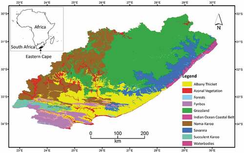
Biomes in South Africa are defined mainly based on floristic characteristics and dominant life or growth forms (Rutherford et al. 2011a). Macroclimatic characteristics that affect the biota are also used as additional criteria in the biome definition. However, it should be noted that climatic data at the biome level (given in Table 1) are indicators of central tendencies at best and may not necessarily represent the variations in the biome (Rutherford et al. 2011a).

The Albany Thicket Biome has characteristics closely related to the Mediterranean forests, woodlands and scrubs category of the global vegetation classification (Hoare et al. 2011). The vegetation consists mainly of dense, woody, semi-succulent and thorny plants such as the Vachellia (formerly Acacia) species. Albany Thicket is considered a species-rich biome that boasts great variation in growth forms. The Fynbos Biome is synonymous with the Cape Floristic Region, experiences the Cape Mediterranean climate and is renowned for its high diversity of species and local endemism (Rebelo et al. 2011). The most common vegetation types in the biome include shrubs of Restionaceae and Asteraceae, as well as sclerophylls. In addition, the biome also has grasses that grow as understorey and in between shrubs. The Grassland Biome is by far the most dominant in the province with a 41.6% spatial coverage (SANBI 2012). It is part of the global Temperate Grassland Biome (Mucina et al. 2011a). Although the Grassland Biome is dominated by graminoids in the province, it also contains shrubs – particularly in areas where the moisture-holding capacity of soils is high (Mucina et al. 2011a). Despite its current spatial coverage, the Grassland Biome is predicted to shrink significantly under increased atmospheric CO₂ emission scenarios (Mucina et al. 2011a). The Savanna Biome forms part of the biome that is found widely in Africa (Rutherford et al. 2011b). Although it has the largest coverage in South Africa, its distribution in the study area is limited to the coastal areas. As a result, the Biome is influenced greatly by climatic patterns of the Atlantic and the Indian Oceans bordering the study area (Rutherford et al. 2011b). The biome has wet summers, dry winters and a low frost occurrence (Rutherford et al. 2011b). The vegetation of the Savanna Biome consists of grass-dominated herbaceous forms interspersed by a varying density of woody plants.

The Nama-Karoo Biome is described in Evenari (1985) and Wegner (1986) as a hot desert; as a result, it is considered an arid biome. Characteristically, the Nama-Karoo has a continental climate with little influence from oceanic systems (Mucina et al. 2011b). Despite its large spatial coverage in the study area (18.8%), the Nama-Karoo is known for low endemism and species diversity due to geological and environmental homogeneity across the biome (Mucina et al. 2011b). A mixture of dwarf shrubs, grasses, succulents, geophytes and forbs dominate the vegetation of the biome (Mucina et al. 2011b). The Succulent Karoo Biome borders the Nama-Karoo Biome, but is situated in a climatically different zone that receives more rain in winter than in summer. Furthermore, the Succulent Karoo has amongst the highest floral diversity among arid environments globally (Mucina et al. 2011c). The most common vegetation units in the Succulent Karoo Biome within the study area include dwarf succulent shrubs and scattered assemblages of thicket (Mucina et al. 2011c).

The Indian Ocean Coastal Belt (IOCB) Biome, which is similar to the Tropical Broadleaved Moist Forest Biome (Burgess et al. 2004), is globally associated with forest, grassland and savanna mixtures (Mucina et al. 2011d). The IOCB is known to display significantly different vegetation structures and climatic characteristics compared to the other biomes considered in our study. The Azonal Vegetation Biome has a relatively small coverage in the province and does not necessarily follow the climatic zonation that is used as one of the criteria in the other zoned biomes (Mucina, Rutherford, and Powrie 2011e). Instead, the Azonal Vegetation Biome is influenced mainly by localized ecological characteristics such as soils, hydrogeology and salinity conditions. It is characterized by salt- and flood-tolerant vegetation types adapted to soil bases experiencing high waterlogging and/or salt concentrations such as in coastal areas or near waterbodies in inland areas (Mucina, Rutherford, and Powrie 2011e). As a result, this biome is distributed within other biomes, indicating little-to-nil zonal requirements for its occurrence. The Forest Biome is the smallest of all biomes, reflecting the national-level statistic. This biome forms part of the African Afro-temperate and Coastal Forests group (White 1983; Timberlake and Shaw 1994). Unlike the other zonal biomes, the Forest Biome rarely follows zonal patterns; instead, it is embedded as patches within or along ecotones of other biomes (Mucina and Geldenhuys 2011; Rutherford et al. 2011a). The Forest Biome is generally dominated by tall, woody plants and different levels of layering, varying from multi-layered trees to trees with shrubby understorey (Mucina and Geldenhuys 2011).

Remote sensing data

Moderate Resolution Imaging Spectroradiometer (MODIS) remote sensing provides different products including multispectral images and processed products such as vegetation indices and land surface temperature at multiple spatial and temporal resolutions. Vegetation indices, namely the Normalized Difference Vegetation Index (NDVI) and the Enhanced Vegetation Index (EVI), analyzed using the Multi-angle Implementation of Atmospheric Correction (MAIAC) algorithm were used in the study. The algorithm applies a time-series analysis and a combination of pixel and image processing on MODIS data acquired by Aqua and Terra satellites to correct for atmospheric interferences. The combination of multi-angle look and atmospheric correction processes results in surface reflectance data that are assumed to be taken at nadir view (Lyapustin and Wang 2018). Eight-day composite NDVI and EVI data with a spatial resolution of 0.05° were downloaded from the National Aeronautics and Space Administration (NASA) Center from Climate Simulation (NCCS) Dataportal. The data used for this study ranged between February 2000 and December 2017. A temporally weighted average was applied to compute the monthly NDVI and EVI from the 8-day composites. The NDVI, which mathematically combines red and near-infrared electromagnetic radiations (Equation 1), is a strong indicator of vegetation conditions, particularly in low-to-moderate vegetation biomass conditions, while it suffers in instances of high vegetation cover (Kogan 1990; Nicholson, Davenport, and Maloa 1990; Graw et al. 2017). In contrast, the EVI (Equation 2) captures the variation better – even in highly vegetated areas (Kogan 1990; Graw et al. 2017). Considering the great variation in vegetation biomass across – and to an extent within – biomes, it is important to compare the performance of the two indices.

(1) $\mathrm{N}\mathrm{D}\mathrm{V}\mathrm{I}=\frac{\left(\mathrm{N}\mathrm{e}\mathrm{a}\mathrm{r}\mathrm{I}\mathrm{n}\mathrm{f}\mathrm{r}\mathrm{a}\mathrm{r}\mathrm{e}\mathrm{d}-\mathrm{R}\mathrm{e}\mathrm{d}\right)}{\left(\mathrm{N}\mathrm{e}\mathrm{a}\mathrm{r}\mathrm{I}\mathrm{n}\mathrm{f}\mathrm{r}\mathrm{a}\mathrm{r}\mathrm{e}\mathrm{d}+\mathrm{R}\mathrm{e}\mathrm{d}\right)}$(1)

(2) $\mathrm{E}\mathrm{V}\mathrm{I}=G\frac{\left(\mathrm{N}\mathrm{e}\mathrm{a}\mathrm{r}\mathrm{I}\mathrm{n}\mathrm{f}\mathrm{r}\mathrm{a}\mathrm{r}\mathrm{e}\mathrm{d}-\mathrm{R}\mathrm{e}\mathrm{d}\right)}{\left(\mathrm{N}\mathrm{e}\mathrm{a}\mathrm{r}\mathrm{I}\mathrm{n}\mathrm{f}\mathrm{r}\mathrm{a}\mathrm{r}\mathrm{e}\mathrm{d}+\mathrm{C}1\ast \mathrm{R}\mathrm{e}\mathrm{d}-\mathrm{C}2\ast \mathrm{B}\mathrm{l}\mathrm{u}\mathrm{e}+\mathrm{L}\right)}$(2)

where G is gain factor equal to 2.5, L is the soil adjustment factor specified at 1, and C1 and C2 are the coefficients used to correct aerosol scattering in the red band by the use of the blue band and are given as 6 and 7.5, respectively.

Monthly MODIS Land Surface Temperature (LST) data at a spatial resolution of approximately 6 km were downloaded for the same period as the NDVI and EVI data. The LST data (MOD11B3 version 6) used in the study was a simple temporal average of daily LST data (MOD11B3) acquired by MODIS sensor onboard Terra satellite. One of the improvements of MOD11B3 version 6 product on the previous versions was the exclusion of cloud-contaminated daily LSTs from computation of the monthly average (Wan 2013). Few missing pixels were observed in certain months; however this did not constitute a concern in our study, since our analysis was based on biome-level spatial mean values. As a crude confirmation of the data, a comparison was made between the MODIS monthly LST and temperature recorded at six meteorological stations (with nearest stations spaced 75–200 km apart) using Pearson’s correlation, r. The correlations (r) ranged between 0.76 and 0.88, with five of the stations having an r of 0.82 or above.

Monthly rainfall data used in this study was obtained from the Climate Hazards Group Infrared Precipitation with Stations (CHIRPS) data collection. We downloaded the gridded CHIRPS Version 2 data at a spatial resolution of 0.05° from the United States Agency for International Development’s (USAID) Famine Early Warning Systems online portal. CHIRPS data combine remotely-sensed data products, spatially interpolated gauged rainfall data and geographical information including elevation, latitude and longitude (Funk et al. 2015). The accuracy of the CHIRPS product is therefore partly dependent on the station network of a given area. A comparison of the CHIRPS data with rainfall data recorded at six weather stations matching the CHIRPS showed a correlation (r) ranging between 0.64 and 0.87, with five of the stations having an r ≥ 0.7.

Spatial aggregation per biome

A spatially-aggregated value was computed for each of the variables per biome. The mean value was used in this study, since we considered it to be more stable than the median, which can change significantly when a value within the sample set changes. The biome-based aggregation resulted in quite a crude approximation – particularly in biomes with large areas and great diversity. Future work could overcome this problem by, for instance, using smaller zones such as bioregions. The biome-aggregated data were then used to build models using a time-series regression modeling approach. A static model and three variants of a distributed lag model were compared in this study, with climatic data serving as explanatory variables and NDVI/EVI as response variables. Details of the modeling exercise are given in the following section.

Statistical analysis

Static model

The main focus of this study was to apply the autoregressive distributed lag (ARDL) model to estimate the NDVI and EVI (response variables) using temperature, precipitation and lagged values of NDVI and EVI as explanatory variables. However, we also applied a static model to contextualize the level of improvement obtained by applying the ARDL model. A static model provides parameter estimates that remain fixed over time. For time-series data comprising three variables: $y_t$, $x_t$ and $z_t$, a static model relating $y_t$ to $x_t$ and $z_t$ is given as:

(3) $y_t={\beta }_0+\beta x_t+\gamma z_t+u_t,\mathrm{f}\mathrm{o}\mathrm{r}t=1,\dots ,n$(3)

where $y_t$ is a vector of time series observations on the dependent variables (NDVI or EVI); $x_t$ and $z_t$ are vectors of observations on the independent or explanatory variables (temperature and precipitation); ${\beta }_0$, $\beta$ and $\gamma$ are unknown fixed (static) regression coefficients to be estimated and $u_t$ is a random error term.

ARDL model

The common approach in assessing the time-varying relationship between vegetation indices and climate data involves linear or non-linear correlation analysis that aims to explore the trend of the two variables (e.g. Ahmed et al. 2017; Tang et al. 2017). For vegetation condition modeling purposes, most studies apply auroregression (or its variants), which uses only the antecedent vegetation condition of interest (endogenous variable) as a predictor (e.g. Guo et al. 2014; Roy and Yan, In press) or a regression analysis that uses temporally-coincident vegetation and climate data (climate being the exogenous variable) as a predictor (e.g. Scanlon et al. 2002; Omuto et al. 2010; Wei et al. 2014). Vegetation has also been related to lagged climate data (e.g. Xu et al. 2011; Barbosa and Lakshmi Kumar 2016; Ahmed et al. 2017). The ARDL approach combines antecedent endogenous and exogenous variables as predictors – in this study, vegetation and climate data respectively. In addition, it allows for including antecedent observations of exogenous variables.

Ideally, the ARDL model should be applied to a set of data series that exhibits stationarity (non-trending behavior) over time. Stationarity was evaluated using the Augmented Dickey-Fuller (ADF) (Dickey and Fuller 1979) and Phillips-Perron (PP) (Phillips and Perron 1988) tests – both of which consider the null hypothesis that the series is non-stationary. Table 2 shows that the ADF and PP values deviated significantly from the null hypothesis (at 5% significance level) in all dependent and independent variables. This indicates stationarity in the time-series process of the data and thus the suitability of the ARDL model for the data.

Table 2. Stationarity test results run on each time-series of data using the ADF and PP tests.

	Temperature		Rainfall		NDVI		EVI
	ADF	PP	ADF	PP	ADF	PP	ADF	PP
Grassland	−9.87**	−6.07**	−12.45**	−7.39*	−10.69**	−7.91**	−11.04**	−7.71**
Succulent Karoo	−9.23**	−6.03**	−9.58**	−12.08**	−8.68**	−10.31**	−7.03**	−10.92**
Savanna	−9.00**	−6.00**	−11.32**	−7.86**	−8.68**	−9.14**	−9.93**	−8.76**
Nama-Karoo	−9.68**	−6.09**	−11.39**	−9.09**	−9.46**	−9.00**	−8.84**	−10.19**
Indian Ocean Coastal Belt	−9.66**	−6.19**	−9.34**	−8.39**	−7.73**	−11.02**	−8.57**	−10.13**
Fynbos	−10.17**	−6.06**	−8.19**	−13.56**	−6.21**	−11.17**	−5.28**	−11.57**
Forest	−10.31**	−6.09**	−9.61**	−8.78**	−7.84**	−10.80**	−8.57**	−9.73**
Azonal Vegetation	−9.01**	−6.05**	−10.45**	−10.93**	−7.47**	−10.49**	−6.55**	−11.23**
Albany Thicket	−9.17**	−6.03**	−9.76**	−11.69**	−6.09**	−9.80**	−6.39**	−10.47**

* and ** denote significance at the 5% and 1% levels, respectively.

The distributed lag model (DLM) has been developed on the principle that lagged values of explanatory variables and current values influence the response variable. The model is defined as:

(4) $y_t=\alpha +{\beta }_0{x}_t+{\beta }_1{x}_{t-1}+{\beta }_2{x}_{t-2}+\dots +{\beta }_k{x}_{t-k}+u_t$(4)

where $\alpha$ is the intercept, ${\beta }_0$ is the immediate impact of the explanatory variable $\left(x\right)$ on a response variable ($y)$, ${\beta }_1$ is the impact of order one-lagged $x$ on y, ${\beta }_2$ is the impact of order two-lagged $x$, and so on.

Furthermore, the dynamic behavior of a dependent variable can be studied by including the lagged values of the dependent variable itself. A model that includes both lagged dependent and independent variables as regressors is called the ARDL (p, q), where p and q denote the number of lags of response and explanatory variables, respectively (Uwe and Jürgen 2005). The ARDL model, therefore, captures the dynamic effects from lagged explanatory and response variables. The ARDL (p, q) can be computed as:

(5) $y_t={\alpha }_0+{\alpha }_1{y}_{t-1}+\dots +{\alpha }_p{y}_{t-p}+{\beta }_0{x}_t+{\beta }_1{x}_{t-1}+\dots +{\beta }_q{x}_{t-q}+u_t$(5)

where ${\alpha }_1,\dots ,{\alpha }_p$ is the magnitude of the effects of past response variables on the current response variable and $u_t$ is a white noise term (i.e. error terms having no heteroscedasticity or autocorrelation). In the case of two explanatory variables such as $x_t$ and $z_t$, the ARDL model can be abbreviated as $ARDL\left(p,q_1,q_2\right)$:

(6) $y_t={\alpha }_0+{\alpha }_1{y}_{t-1}+\dots +{\alpha }_p{y}_{t-p}+{\beta }_0{x}_t+{\beta }_1{x}_{t-1}+\dots +{\beta }_{q_1}{x}_{t-q_1}+{\gamma }_0{z}_t+{\gamma }_1{z}_{t-1}+\dots +{\gamma }_{q_2}{z}_{t-q_2}+u_t$(6)

where $p,q_1$ and $q_2$ denote the number of lags of y, x and z, respectively.

We initially compared four different lag orders including 2-, 3-, 6- and 12- lags to estimate the NDVI and EVI, and found the improvement in root mean square (RMSE) between 2-lags and any of the other lags to be a maximum of 4%. We decided to limit the lag in the estimation of both the EVI and NDVI to two months only. Note that ARDL (1,1,1) and ARDL (2,2,2) are represented by ARDL1 and ARDL2, respectively. In the present study, we fitted and compared ARDL1 and ARDL2 models against the Koyck and static models.

Distributed lag models with Koyck transformation

The Koyck model (Koyck 1954) assumes that the current value of a dependent variable in a time-series process is influenced by current explanatory variables as well as infinite number of lagged explanatory variables, given as:

(7) $y_t=\alpha +\sum _{i=0}^{\mathrm{\infty }}{\beta }_i{x}_{t-i}+u_t$(7)

The model theoretically quantifies an infinite number of $\beta$ (weights of lagged, explanatory variables), by assuming an unlimited number of time lags. However, the weights of lagged, explanatory variables ($\beta$) do not bear the same impact; instead, they decrease with time. It is suggested that the impacts have a systematic similarity that decreases with time lapsed at a geometrical rate given as: ${\beta }_i=\beta {\varphi }^i$, $\left|\varphi \right|<1$. This process makes the impact of remote past factors on current responses insignificant. To avoid impractical computations of all past effects, the model suggests subtracting the product of the decrease rate ($\varphi$) and the immediate past dependent variable ($y_{t-1}$) from the current, dependent variable ($y_t$) given as:

$y_t-\varphi y_{t-1}=\alpha \left(1-\varphi \right)+\beta x_t+(u_t-\varphi u_{t-1}).$

Solving this equation results in model (8):

(8) $y_t=\alpha \left(1-\varphi \right)+\beta x_t+\varphi y_{t-1}+(u_t-\varphi u_{t-1})={\beta }_1+{\beta }_2{y}_{t-1}+{\beta }_3{x}_t+v_t$(8)

where${\beta }_1=\alpha \left(1-\varphi \right)$,${\beta }_2=\varphi$, ${\beta }_3=\beta$ and $v_t=u_t-\varphi u_{t-1}$.

Note that subtracting from the previous dependent variable includes the associated error, too (Hill, Griffiths, and Judge 2000). It can be argued the Koyck transformation converted the distributed lag model into an autoregressive model that relies on current explanatory variable(s) and immediate lag of the dependent variable. It is mandatory to confirm that the estimation errors (u_t) resulting from the above models do not exhibit serial correlations (autocorrelation); that is, errors between consecutive estimations should not have similar/comparable values (Durbin and Watson 1950). The Durbin-Watson (DW) test (Durbin and Watson 1950) is one of the most commonly used methods for testing the presence of autocorrelation (Lewis-Beck, Bryman, and Liao 2004). This is a standard test that does not rely on a large sample size approximation (Durbin and Watson 1950; Montgomery, Peck, and Vining 2001). The hypotheses considered in the DW test include $H_0:\rho =0$ representing no autocorrelation, versus presence of autocorrelation denoted as $H_1:\rho >0$, where ρ is the first order autocorrelation, i.e. correlation between two consecutive time points (in our case, months). The test statistic is quantified as $DW\approx 2\left(1-\hat{\rho }\right)$, where $\hat{\rho }$ is the estimated first order autocorrelation. If $\hat{\rho }\approx 0$, then the DW statistic is closer to 2, which is an indication that model errors are not autocorrelated. In contrast, $\hat{\rho }>0$ implies that the DW statistic is less than 2, suggesting the presence of autocorrelation (Montgomery, Peck, and Vining 2001).The presence of autocorrelation in the time-series data also compromises the reliability of the significance level of parameter estimates due to incorrect standard errors. Therefore, correcting the standard error post-modeling aids in confidently determining whether the model and parameter estimates are significant. In this study, we applied the Newey-West method (Newey and West 1987) to correct the standard errors of serially correlated errors.

Goodness-of-fit statistics

In the context of the dynamic linear regression model (2), we chose $p,q_1$ and $q_2$ that minimized the Sum-of-Squared-Errors (SSE). For the present study, model fitness was evaluated based on the coefficient of determination (R²), RMSE, while Akaike Information Criterion (AIC), the Bayesian Information Criterion (BIC) and the log-likelihood function were used to rank candidate models. The AIC measures the distance between a fitted model and an ideal but unknown model that generated the data. The AIC (Akaike 1974) is computed by Equation 9:

(9) $AIC=ln\left(\frac{SSE}{n}\right)+\frac{2k}{n}$(9)

where k is the number of regression coefficients that are estimated, including the intercept, SSE is the Sum-of-Squared-Errors and n is the number of samples/observations. Similarly, the BIC (Schwarz 1978) is given by Equation 10. The BIC penalizes additional lags more heavily than does the AIC, since $\frac{kln\left(n\right)}{n}>\frac{2k}{n}$ for $n\ge 8$ (in this case, n is 216). Models with lower AIC and BIC values and higher log-likelihood values are favored over those with higher values. The BIC is computed by Equation 10:

(10) $BIC=ln\left(\frac{SSE}{n}\right)+\frac{kln\left(n\right)}{n}$(10)

It is useful to use additional model selection techniques to strengthen the conclusion on the fit quality of a modeling exercise. This is particularly relevant to avoid over-reliance on the goodness-of-fit statistics noted above (R², RMSE, AIC, BIC, log-likelihood); these statistical tools may, in certain instances, not capture the detailed variability present. While the goodness-of-fit statistics basically quantify the degree of association between explanatory and response variables, we carried out a further analysis using estimation errors. Apart from the intrinsic importance of quantifying error levels, this approach also aids in the comparison between models. In this study, we compared the error levels between the best model and the other, inferior models using a pairwise analysis to determine the difference between the two. Such a comparison based on errors reduces the dependence solely on standard goodness-of-fit statistics that show aggregate information while hiding important information of individual samples.

Results

Model goodness-of-fit statistics including R² and RMSE are shown in Figure 2, while detailed statistics as well as selection and comparison between models for all approaches per biome are given in Table S1. Note that the distributed lag models (including Koyck, ARDL1 and ARDL2) had better R² for all biomes than did the static model. In addition, the lower AIC and BIC values and higher log-likelihood (LogLik) statistic of the distributed lag models compared to the static model confirmed the superiority of the former (Table S1). A closer comparison among the distributed lag models showed the superiority of the model that utilized up to two lagged months of the climate and the dependent variables (ARDL2) while the Koyck-transformed distributed lag model had the lowest accuracies for all biomes.

Figure 2. R² and %RMSE statistics of the four models used to estimate NDVI and EVI values per biome.

A relative comparison of the fitted models among biomes shows Grassland followed by Nama-Karoo and Savanna to have the best NDVI estimations, particularly using the ARDL1 and ARDL2 models, based on R². Generally, similar observations but with lower R² and higher percent RMSE were observed for EVI estimations in six of the nine biomes. In particular, the R² for the NDVI estimation was 10% or greater than for the EVI in Succulent Karoo, Nama-Karoo, Fynbos and Azonal Vegetation Biomes. In contrast, R² was better for EVI than NDVI estimation in the Forest and Indian Ocean Coastal Belt Biomes.

A closer per-biome observation was made based on the model characteristics of the ARDL2 model, which yielded the best fit based on model goodness-of-fit statistics given in Figure 2. It is important, however, to verify that estimation residuals do not suffer from serial correlation. The results of the serial correlation test using the DW test showed no serial correlation in estimation residuals of NDVI. Residuals of EVI estimation were serially correlated in the Fynbos Biome (DW = 1.74, p_(α:5%) = 0.021); therefore, corrections were applied to this biome.

Subsequently, model characteristics to estimate the current NDVI and EVI using the ARDL2 approach were undertaken (see Table 3). Current temperature (Temp_t) had a negative impact on NDVI in all biomes but it was statistically significant in one biome only (Indian Ocean Coastal Belt). Current precipitation (Precip_t) had a positive impact on NDVI; however, it was significant in the Savanna and Forest Biomes only. The effect of temperature of one-month lag (Temp_t−1) was not significant in all but one biome (Nama-Karoo Biome). In contrast, one-month lagged precipitation (Precip_t−1) had a statistically significant impact on the NDVI in all biomes. Temperature lagged by two months (Temp_t-2) had a positive effect on the NDVI in all biomes but was significant only in Grassland and Indian Ocean Coastal Belt Biomes. A two-month lagged precipitation (Precip_t−2) was a significant predictor of the NDVI in almost all biomes. The NDVI lagged by one month (y_t−1) was a significant predictor of the NDVI in most biomes. In contrast, the NDVI lagged by two months (y_t−2) had a significant effect in three biomes only (Succulent Karoo, Fynbos, Azonal Vegetation).

Table 3. Parameter estimates for modeling NDVI and EVI using ARDL2 model per biome. The standard errors are reported in parentheses.

	NDVI
Biomes	Intercept	Tempt	Precipt	Tempt-1	Precip t-1	Temp t-2	Precip t-2	y t-1	y t-2
Grassland	−0.094	−17.2987	0.00004	−30.8056	0.0012**	0.2132*	68.5809**	0.0007**	0.0345
Succulent Karoo	0.9333**	−34.1828	0.0001	−22.5591	0.0015**	0.1154	3.4348**	0.0007	0.145*
Savanna	0.1918	−46.0487	−0.00003**	−17.0784	0.0011*	0.2053	67.6383**	0.0007**	0.1099
Nama-Karoo	0.5991**	−4.3400	0.0003	−56.5101*	0.0013**	0.1494	30.8093*	0.0005	0.0679
Indian Ocean	0.1451	−223.838**	−0.0002	71.3867	0.0007**	0.1153*	170.7327*	0.0005	0.0792
Fynbos	1.062**	−67.909	−0.0003	−20.9831	0.0007**	0.2313	35.6315	0.0003**	0.1619*
Forest	−0.3179	−99.9269	−0.0005*	63.4228	0.0009**	0.1975	85.2382*	0.0005**	0.0716
Azonal Vegetation	0.6133**	−4.2407	0.0001	−58.0946	0.0013**	0.1679	32.5833**	0.0006*	0.1211*
Albany Thicket	1.0964**	−25.3299	0.0001	−88.2586	0.0016**	0.3142	54.7089**	0.0006**	0.0564
	EVI
Biomes	Intercept	Tempt	Precipt	Tempt-1	Precip t-1	Temp t-2	Precip t-2	y t-1	y t-2
Grassland	−0.3119	−9.6106	−0.00002	7.7634	0.0008**	0.119	28.8701**	0.0004**	0.0386
Succulent Karoo	0.2664**	−12.1643	−0.00002	0.3178	0.0008**	0.1688	−2.7104**	0.0004*	0.2396**
Savanna	−0.1917	−13.2054	−0.00004	11.8786	0.0009**	0.1731	22.6891**	0.0006*	0.1123
Nama-Karoo	0.1592	−0.9779	0.0001	−15.6331	0.0008**	0.0772	11.0228*	0.0003	0.0873
Indian Ocean	−0.4759*	−165.045	−0.0001	120.6768	0.0007**	0.131	90.6073*	0.0004	0.083
Fynbos	0.2801	−24.5	−0.0004**	21.0539	0.0004**	0.2572	−5.9704	0.0002**	0.1328*
Forest	−1.0757*	−33.937	−0.0004*	93.6059	0.0009**	0.202	25.2564**	0.0005**	0.1027
Azonal Vegetation	0.0475	9.0189	−0.0001	−17.4932	0.0009**	0.1659	11.055	0.0004*	0.1149
Albany Thicket	0.3449	3.7414	−0.0002	−41.7516	0.0012**	0.2602	23.1529*	0.0004**	0.0291

* and ** denote significance at the 5% and 1% levels, respectively. Temp and Precip are independent variables representing temperature and precipitation, respectively; y = dependent variable (NDVI or EVI); t-1 and t-2 represent first and second lags, respectively.

Looking at parameter estimates for EVI modeling, there were similarities with the NDVI estimation in a general sense (Table 3). For example, current temperature (Temp_t) did not have a significant effect on EVI in all biomes, while current precipitation (Precip_t) had a significant impact on EVI only in the Fynbos and Forest Biomes. Similarities with NDVI estimation were also observed in the impacts of one-month-lagged and two- month-lagged temperature and precipitation in many of the biomes. Like the NDVI estimation, one-month lagged EVI values (y_t−1) had a significant impact on current EVI in most biomes, while EVI lagged by two months (y_t−2) was a significant predictor in two biomes only (Succulent Karoo, Fynbos).

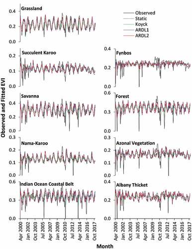
Plotting observed and fitted values generates a visual representation providing an opportunity for insightful interpretation into the time series processes not conveyed through goodness-of-fit and other empirical statistics. Figures 3 and 4 plot these processes using estimates generated by the four models (static, Koyck, ARDL1 and ARDL2). Note that the comparison between the different models starts from April 2000, since the two-month-lag specification resulted in no ARDL2 model for the first two months (February and March 2000). Generally, the plots show how closely estimated values using the distributed lag models (Koyck, ARDL1 and ARDL2) follow the observed NDVI and EVI values, respectively. In contrast, estimations using the static model lack variations that follow the fluctuation patterns of observed values in all biomes. The graphs also show differences in fluctuation complexity of the time-series processes among biomes. Grassland, Savanna, Indian Ocean Coastal Belt, and Forest Biomes have a more regular fluctuation pattern compared to the other biomes. Despite these differences, the distributed lag models were better than the static model at representing both the NDVI (Figure 3) and EVI (Figure 4).

Figure 3. Observed and fitted monthly NDVI values per biome level between April 2000 and December 2017.

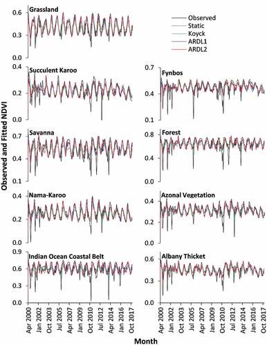
Figure 4. Observed and fitted monthly EVI values per biome level between April 2000 and December 2017.

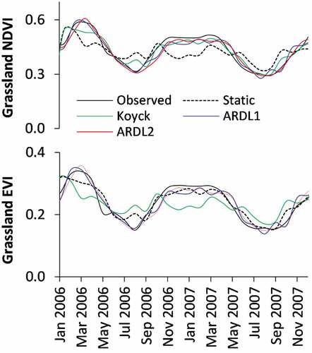
It is important to note differences among the distributed lag models. We selected a time-period between January 2006 and December 2007, when both the NDVI and EVI of Grassland Biome fluctuate considerably, to illustrate the relative differences between the three distributed lag models (Figure 5). The static and Koyck models fits poorly when the NDVI and EVI were high in March 2006, and low in August 2006. Poor fits are also observed when using the static model between November 2006 and May 2007 to estimate NDVI, while this problem is noted for EVI estimation during the same period using the Koyck model. Although the ARDL1 and ARDL2 were generally comparable, the former showed more fluctuations as opposed to the rather constant NDVI and EVI observations of ARDL2 during November 2006–May 2007.

Figure 5. Differences between the fitted models in NDVI and EVI estimation focusing on the period January 2006– December 2007.

Considering the superiority of the ARDL2 model (Figures 2–5), we used the ARDL2 model as the benchmark against which the others were compared to determine the level of equivalence between estimation residuals, as shown in Figure 6 (NDVI) and Figure 7 (EVI). Please note that the static model was not included in the pairwise comparison in Figures 6 and 7, as it was deemed quite weak based on the other statistics as well as from observations drawn from Figures 2–5. We included Pearson’s correlation coefficient (r) in the comparisons of the residuals. The ideal similarity between estimation errors of two models would give an r of 1. In all cases, the best model (ARDL2) had better comparability with ARDL1 than with the Koyck model. Interestingly, the error comparisons show insights that are missed by the other goodness-of-fit statistics. In general, the estimation residuals of the three models (Koyck, ARDL1 and ARDL2) showed good similarities in terms of magnitude and direction of errors for both NDVI and EVI. It is important to note that these similarities were stronger than the estimation accuracies of individual models reported in Figure 2. For example, the residual correlations between ARDL2 and Koyck in the Azonal Vegetation Biome (r: 0.86 for NDVI and r: 0.88 for EVI) were better than the R² differences between the same models in Figure 2 (0.23 vs. 0.44 for NDVI; 0.09 vs. 0.30 for EVI). Similar observations can be made in the Succulent Karoo Biome.

Figure 6. Correspondence of NDVI estimation errors of the Koyck and ARDL1 model against estimation errors of ARDL2 per biome. Note that ARDL2 was used as the benchmark based on results reported in Figures 2–5 and Table S1.

Figure 7. Correspondence of EVI estimation errors of the koyck and ARDL1 model against estimation errors of ARDL2 per biome. Note that ARDL2 was used as the benchmark based on results reported in Figures 2–5 and Table S1.

Discussion

Biome vs. estimation accuracy

The present study aimed to investigate the relationship between climatic data and vegetation indices represented by the NDVI and the EVI using a time-series analysis at the biome level. Each of the biomes represents a complex vegetation-climatic composition () inherently associated with different growth patterns. Generally, the results showed the ability of current and lagged climatic variables (temperature, precipitation) as well as lagged dependent variables (NDVI and EVI, respectively) to estimate NDVI and EVI for a given time. The significant effect of precipitation on NDVI or EVI found in this study (Table 3) agrees with other studies conducted in (semi-) arid environments (e.g. Wen, Yang, and Saintilan 2012; Tang et al. 2017; Zhang et al. 2017). The similarity with the findings by Tang et al. (2017) is particularly notable in that NDVI had a stronger correlation with lagged precipitation than with temperature in forest, cropland and grassland cover types. Their study, however, was limited to correlation analysis compared to ours, which was aimed at generating estimation models. Estimation accuracies compare favorably with other studies, despite methodological and floral composition differences. For example, Li et al. (2013) correlated MODIS NDVI of growing season and accumulated precipitation in grassland pastures, and achieved an R² = 0.97 compared to 0.78 in our case, where the biome is more complex in species composition.

Relative comparison of goodness-of-fit statistics of NDVI and EVI estimations among biomes were best in Grassland, Savanna and Nama-Karoo Biomes (Figure 2). This is expected because each of these vegetation types has fairly homogenous structures and high vegetation cover. In spite of the coarse spatial resolution, MODIS-derived NDVI and EVI are therefore representative of the vegetation conditions in these biomes. Climatic patterns of these biomes are also predictable and influence the vegetation patterns considerably (Rutherford et al. 2011a). The combination of these two characteristics results in strong correlations between climate and vegetation cover. The other biomes have more complicated vegetation structures that may not match the spatio-temporal variation of climate data. For example, it is common to find considerable differences in vegetation types or structure within a given small area that experiences a single set of climatic characteristics. Such a mismatch leads to a weak relationship between vegetation and climate.

The Nama-Karoo Biome is dominated by dwarf plants of limited diversity that can tolerate a predominately hot environment with low precipitation (Table 1). Logically, the overall coverage of plants in such environments is low, as a result of moisture scarcity coupled with overgrazing over a long period of time in the region (Mucina et al. 2011b). There is a strong likelihood that the spatial resolution of the MODIS image is coarse and thus unable to accurately capture the amount of vegetation in the biome. This could make a significant contribution to the low NDVI (~0.2–0.4) and EVI (~0.1–0.2) values observed in Figures 3 and 4, respectively. On the other hand, the climate data show more variation, including high precipitation occurrences and low temperatures, that is often unpredictable and short-lived (Mucina et al. 2011b). Furthermore, the weakly-structured soil conditions symptomatic of the biome (Mucina et al. 2011b) imply low moisture holding capacity in rainy periods. Such a mismatch results in correlations between climate and vegetation that, at times, are weak.

The weak correlations observed in the Succulent Karoo Biome, compared to the Nama-Karoo Biome, are expected given the nature of the plants that dominate the biome. Specifically, succulent plants conserve moisture for relatively long periods of time, maintaining a good deal of greenness that may run well into dry seasons. While the relationship between the vegetation greenness (through NDVI and EVI) and climatic variables is expected to be solid during optimal growth periods, it decreases during other seasons when precipitation is low.

Model comparison and implications

Structural differences exist between the ARDL models and the Koyck-transformed distributed lag model in that the latter relies on current values of independent variables (temperature and precipitation) and past values of the dependent variable. However, all these models appear to yield comparable estimation accuracies (see %RMSE in Figure 2) that could be attributed to the impact of lagged NDVI and EVI values. With the ARDL2 model the reference as the best model (Figure 2), the ARDL1 was found to be better than the Koyck-transformed model (Figures 6 and 7). This indicates the importance of the lagged independent variables used by the ARDL models.

Looking at ARDL1 and ARDL2 models using error correspondence for each biome indicates strong similarities between the two models in all biomes (Figures 6 and 7). It is particularly important to notice the similarities between the Azonal Vegetation, Albany Thicket and Fynbos Biomes which are quite complex in terms of vegetation structures, as can be noted by the relatively high number of bioregional–vegetation type compositions (Table 1). The complexity in vegetation forms, species compositions and growth stages increases the potential of phenological complexity and overlap in a given biome (Kimball 2014; Thompson et al. 2017). This, therefore, reduces the cumulative difference between one- and two-month lags (ARDL1 and ARDL2, respectively).

The similarities of ARDL1 and ARDL2 in the Nama-Karoo are influenced by a combination of vegetation and climate characteristics. Nama-Karoo is an arid zone characterized by hot, dry temperature levels and limited precipitation that combine to support low-statured shrubs (Mucina et al. 2011b). Such vegetation is accompanied by low biodiversity with only three vegetation types found in the province (Table 1). Furthermore, the overall vegetation cover of this biome is considered low as can be seen from the low NDVI and EVI variations in Figure 3, though the coarse spatial resolution of MODIS also contributes to these variations. A combination of these factors – driven by prolonged spells of harsh environments (Mucina et al. 2011b) – makes the effects of the two lags on current estimates similar. Equivalence of ARDL1 and ARDL2 in the Succulent Karoo is attributed primarily to the vegetation type dominating in the biome. The high moisture-holding capacity of succulent plants for prolonged periods ensures plant greenness even into dry spells, resulting in similar effects for the two lag times considered by ARDL1 and ARDL2.

Ecological significance of ARDL2 models

The importance of lagged climatic factors on vegetation has been demonstrated in previous studies (Guo et al. 2014; Wu et al. 2015; Barbosa and Lakshmi Kumar 2016) including in African savanna (Tsalyuk, Kelly, and Getz 2017). The effect of lagged climatic variables on “current” vegetation may depend on a number of factors such as vegetation type, growth stage or phase and climatic conditions (Schmidt and Karnieli 2000). Using analysis of global data, Wu et al. (2015) revealed that time-lag effects of climatic factors can vary even for the same vegetation type. It is, therefore, unlikely to find a definitive lag size for a biome-level assessment since a typical biome, like the ones used in our study, consists of various vegetation types. Potential phenological differences among these vegetation types can also complicate the determination of a lag size that fits all vegetation types. Initial comparison of multiple lags in our study resulted in limited difference beyond the 2-month lag. This, however, does not preclude the potential for a better result using more lag sizes, as for example illustrated by Barbosa and Lakshmi Kumar (2016), who found the best correlation between NDVI and 3-month lagged rainfall data in a dryland vegetation type. We believe that the 2-month lag used in our study is a good compromise as using a higher lag size may result in straddling between seasons. That is, it would be inappropriate to correlate the current vegetation amount with vegetation and climate data of a different season.

Room for improvement

The findings of this study are promising with accuracies and goodness-of-fit statistics comparable with the literature, despite our focus on biomes that are considered complex in terms of vegetation conditions. This study can be improved upon in different ways. Firstly, the use of mean values of variables (NDVI, EVI, precipitation and temperature) per biome are a somewhat crude representation of the biomes. In this regard, Fu and Burgher (2015) classified their study area based on NDVI values in an attempt to capture species complexity. However, it should be kept in mind that NDVI and EVI variation is not necessarily a reflection of species variation; instead, the variation can also be induced by factors such as growth characteristics and plant vigour/senescence. Another alternative can be to subdivide a biome into vegetation units, which can then be related with remotely-sensed data of appropriate spatial resolution. Secondly, precipitation and temperature are only some of the climatic variables that influence vegetation growth. Other variables such as soil moisture (e.g. Ahmed et al. 2017), surface water and groundwater (Fu and Burgher 2015) have been shown to be important determinants of vegetation growth. Therefore, exploring these and other variables will provide a solid base from which reliable information can be drawn about current and forecast vegetation patterns.

Conclusion

The present study sought to build the relationships between vegetation indices and climatic variables at the biome-level. Distributed lag models that utilized either up to one- or two-month lag of climate data and NDVI and EVI yielded generally solid accuracies and better goodness-of-fit statistics in estimating current NDVI and EVI. Estimation accuracies, based on model diagnostics, were particularly high for Grassland, Savanna, Nama-Karoo and to a lesser extent the Forest Biomes primarily due to relative dominance of certain species and corresponding predictability of climatic variables in these biomes. Comparison of models that utilized up to one-month lag (ARDL1) and two-month lag (ARDL2) using error correspondence showed reasonable similarities between the two models (Figures 5 and 6). Overall, these findings show the correlation that exists between climate data and vegetation indices aggregated at the biome-level, even though a biome can comprise complex vegetation types as is the case in South Africa.

Acknowledgements

The University of Johannesburg (South Africa) provided the necessary material support to undertake the study. We thank the National Research Foundation (NRF) of South Africa for partly supporting the first author through student scholarship program. We very much appreciate the four anonymous reviewers whose constructive and critical comments improved the quality of the paper.

Disclosure Statement

No potential nflict of interest was reported by the authors.

Additional information

Funding

This research was funded by the University of Johannesburg.

References

- Ahmed, M., B. Else, L. Eklundh, J. Ardö, and J. Seaquist. 2017. “Dynamic Response of NDVI to Soil Moisture Variations during Different Hydrological Regimes in the Sahel Region.” International Journal of Remote Sensing 38: 5408–5429. doi:10.1080/01431161.2017.1339920.
- Akaike, H. 1974. “New Look at the Statistical Model Identification.” IEEE Transactions on Automatic Control 19: 716–723. doi:10.1109/TAC.1974.1100705.
- Balaghi, R., B. Tychon, H. Eerens, and M. Jlibene. 2008. “Empirical Regression Models Using NDVI, Rainfall and Temperature Data for the Early Prediction of Wheat Grain Yields in Morocco.” International Journal of Applied Earth Observation and Geoinformation 10: 438–452. doi:10.1016/j.jag.2006.12.001.
- Barbosa, H. A., and T. V. Lakshmi Kumar. 2016. “Influence of Rainfall Variability on the Vegetation Dynamics over Northeastern Brazil.” Journal of Arid Environments 124: 377–387. doi:10.1016/j.jaridenv.2015.08.015.
- Birtwistle, A. N., M. Laituri, B. Bledsoe, and J. M. Friedman. 2016. “Using NDVI to Measure Precipitation in Semi-arid Landscapes.” Journal of Arid Environments 131: 15–24. doi:10.1016/j.jaridenv.2016.04.004.
- Boschetti, M., F. Nutini, P. A. Brivio, E. Etienne Bartholomé, D. Stroppiana, and A. Hoscilo. 2013. “Identification of Environmental Anomaly Hot Spots in West Africa from Time Series of NDVI and Rainfall.” ISPRS Journal of Photogrammetry and Remote Sensing 78: 26–40. doi:10.1016/j.isprsjprs.2013.01.003.
- Bradley, B. A., and J. F. Mustard. 2006. “Characterizing the Landscape Dynamics of an Invasive Plant and Risk of Invasion Using Remote Sensing.” Ecological Applications 16: 1132–1147. doi:10.1890/1051-0761(2006)016[1132:CTLDOA]2.0.CO;2.
- Burgess, N., H. D’Amico, J. Underwood, E. Dinerstein, D. Olson, I. Itoua, J. Schipper, T. Ricketss, and K. Newman. 2004. Terrestrial Ecoregions of Africa and Madagascar—a Conservation Assessment. Washington: Island Press.
- Chamaille‐Jammes, S., H. Fritz, and F. Murindagomo. 2006. “Spatial Patterns of the NDVI–rainfall Relationship at the Seasonal and Interannual Time Scales in an African Savanna.” International Journal of Remote Sensing 27: 5185–5200. doi:10.1080/01431160600702392.
- Chen, A., B. He, H. Wang, L. Huang, Y. Zhu, and A. Lv. 2015. “Notable Shifting in the Responses of Vegetation Activity to Climate Change in China.” Physics and Chemistry of the Earth 87–88: 60–66. doi:10.1016/j.pce.2015.08.008.
- Chu, D., L. Lu, and T. Zhang. 2007. “Sensitivity of Normalized Difference Vegetation Index (NDVI) to Seasonal and Interannual Climate Conditions in the Lhasa Area, Tibetan Plateau, China.” Arctic, Antarctic, and Alpine Research 39: 635–641. doi:10.1657/1523-0430(07-501)[CHU]2.0.CO;2.
- Crespo-Mendes, N., A. Laurent, H. H. Bruun, and M. Z. Hauschild. 2019. “Relationships between Plant Species Richness and Soil pH at the Level of Biome and Ecoregion in Brazil.” Ecological Indicators 98: 266–275. doi:10.1016/j.ecolind.2018.11.004.
- Dickey, D. A., and W. A. Fuller. 1979. “Distribution of the Estimators for Autoregressive Time Series with a Unit Root.” Journal of American Statistical Association 74: 427–431.
- Ding, M., Q. Chen, L. Li, Y. Zhang, Z. Wang, L. Liu, and X. Sun. 2016. “Temperature Dependence of Variations in the End of the Growing Season from 1982 to 2012 on the Qinghai–Tibetan Plateau.” GIScience & Remote Sensing 53: 147–163. doi:10.1080/15481603.2015.1120371.
- Durbin, J., and G. Watson. 1950. “Testing for Serial Correction in Least Squares Regression.” Biometrika 37: 409–428.
- Eckert, S., F. Hüsler, H. Liniger, and E. Hodel. 2015. “Trend Analysis of MODIS NDVI Time Series for Detecting Land Degradation and Regeneration in Mongolia.” Journal of Arid Environments 113: 16–28. doi:10.1016/j.jaridenv.2014.09.001.
- Eklundh, L., T. Johansson, and S. Solberg. 2009. “Mapping Insect Defoliation in Scots Pine with MODIS Time-series Data.” Remote Sensing of Environment 113: 1566–1573. doi:10.1016/j.rse.2009.03.008.
- Evenari, N. E. 1985. “The Desert Environment.” In ‘Ecosystems of the World’ (12A), Hot Deserts and Arid Shrublands, edited by M. Evenari, I. Noy-Meir, and D. W. Goodall, 1–22. Amsterdam: Elsevier.
- Fu, B., and I. Burgher. 2015. “Riparian Vegetation NDVI Dynamics and Its Relationship with Climate, Surface Water and Groundwater.” Journal of Arid Environments 113: 59–68. doi:10.1016/j.jaridenv.2014.09.010.
- Funk, C., P. Peterson, M. Landsfeld, D. Pedreros, J. Verdin, S. Shukla, G. Husak, et al. 2015. “The Climate Hazards Infrared Precipitation with Stations—a New Environmental Record for Monitoring Extremes.” Scientific Data. doi:10.1038/sdata.2015.66.
- Graw, V., G. Ghazaryan, K. Dall, A. D. Gómez, A. Abdel-Hamid, A. Jordaan, R. Piroska, et al. 2017. “Drought Dynamics and Vegetation Productivity in Different Land Management Systems of Eastern Cape, South Africa—A Remote Sensing Perspective.” Sustainability 9: 1728. doi:10.3390/su9101728.
- Guo, W., X. Ni, D. Jing, and S. Li. 2014. “Spatial-temporal Patterns of Vegetation Dynamics and Their Relationships to Climate Variations in Qinghai Lake Basin Using MODIS Time-series Data.” Journal of Geographical Sciences 24: 1009–1021. doi:10.1007/s11442-014-1134-y.
- Higgins, S. I., R. Buitenwerf, and G. R. Moncrieff. 2016. “Defining Functional Biomes and Monitoring Their Change Globally.” Global Change Biology 22: 3583–3593. doi:10.1111/gcb.2016.22.issue-11.
- Hill, R. C., W. E. Griffiths, and G. G. Judge. 2000. Undergraduate Econometrics. New York: Wiley.
- Hoare, D. B., L. Mucina, M. C. Rutherford, J. H. J. Vlok, D. I. W. Euston-Brown, A. R. Palmer, L. W. Powrie, et al. 2011. “Albany Thicket Biome.” In The Vegetation of South Africa, Lesotho and Swaziland, Strelitizia 19. L. Mucina and M. C. Rutherford edited by, 540–567. Pretoria: South African National Biodiversity Institute (SANBI).
- Holm, A. M. R., S. W. Cridland, and M. L. Roderick. 2003. “The Use of Time-integrated NOAA NDVI Data and Rainfall to Assess Landscape Degradation in the Arid Shrubland of Western Australia.” Remote Sensing of Environment 85: 145–158.
- https://earlywarning.usgs.gov/fews/datadownloads/Global/CHIRPS%202.0
- https://portal.nccs.nasa.gov/datashare/maiac/DataRelease/Global-VI-8day-0.05degree/
- Ichii, K., A. Kawabata, and Y. Yamaguchi. 2002. “Global Correlation Analysis for NDVI and Climatic Variables and NDVI Trends: 1982–1990.” International Journal of Remote Sensing 23: 3873–3878. doi:10.1080/01431160110119416.
- Jahan, N., and T. Y. Gan. 2011. “Modelling the Vegetation–climate Relationship in a Boreal Mixed Wood Forest of Alberta Using Normalized Difference and Enhanced Vegetation Indices.” International Journal of Remote Sensing 32: 313–335. doi:10.1080/01431160903464146.
- Jiang, L., G. Jiapaer, A. Bao, H. Guo, and F. Ndayisaba. 2017. “Vegetation Dynamics and Responses to Climate Change and Human Activities in Central Asia.” Science of the Total Environment 599–600: 967–980. doi:10.1016/j.scitotenv.2017.05.012.
- Joiner, J., Y. Yoshida, M. Anderson, T. Holmes, C. Hain, R. Reichle, R. Koster, E. Middleton, and F.-W. Zeng. 2018. “Global Relationships among Traditional Reflectance Vegetation Indices (NDVI and NDII), Evapotranspiration (ET), and Soil Moisture Variability on Weekly Timescales.” Remote Sensing of Environment 219: 339–352. doi:10.1016/j.rse.2018.10.020.
- Kawabata, A., K. Ichii, and Y. Yamaguchi. 2001. “Global Monitoring of Interannual Changes in Vegetation Activities Using NDVI and Its Relationships to Temperature and Precipitation.” International Journal of Remote Sensing 22: 1377–1382. doi:10.1080/01431160119381.
- Kim, Y. 2013. “Drought and Elevation Effects on MODIS Vegetation Indices in Northern Arizona Ecosystems.” International Journal of Remote Sensing 34: 4889–4899. doi:10.1080/2150704X.2013.781700.
- Kimball, J. S. 2014. “Vegetation Phenology.” In Encyclopedia of Remote Sensing. E.G. Njoku edited by, 886–890. New York: Springer.
- Kogan, F. N. 1990. “Remote Sensing of Weather Impacts on Vegetation in Non-homogeneous Areas.” International Journal of Remote Sensing 11: 1405–1419. doi:10.1080/01431169008955102.
- Koyck, L. M. 1954. “Distributed Lags and Investment Analysis.” Amsterdam: North-Holland Publishing Co.111 pp.
- Kumar, D., and S. Scheiter. 2019. “Biome Diversity in South Asia - How Can We Improve Vegetation Models to Understand Global Change Impact at Regional Level?” Science of the Total Environment 671: 1001–1016. doi:10.1016/j.scitotenv.2019.03.251.
- Lewis-Beck, M. S., A. Bryman, and T. F. Liao. 2004. “Durbin-Watson Statistic.” The SAGE Encyclopedia of Social Science Research Methods. doi: 10.4135/9781412950589.n261.
- Li, Z., T. Huffman, B. McConkey, and L. Townley-Smith. 2013. “Monitoring and Modeling Spatial and Temporal Patterns of Grassland Dynamics Using Time-series MODIS NDVI with Climate and Stocking Data.” Remote Sensing of Environment 138: 232–244. doi:10.1016/j.rse.2013.07.020.
- Liu, X., and Z. Ren. 2012. “Vegetation Coverage Change and Its Relationship with Climate Factors in Northwest China.” Scientia Agricultura Sinica 45: 1954–1963.
- Lyapustin, A., and Y. Wang. 2018. “MODIS Multi-Angle Implementation of Atmospheric Correction (MAIAC) Data User’s Guide.” Collection 6 (Version): 2.
- MacDonald, G. M., K. D. Bennett, S. T. Jackson, L. Parducci, F. A. Smith, J. P. Smol, and K.J. Willis. 2008. “Impacts of Climate Change on Species, Populations and Communities: palaeobiogeographical insights and frontiers. Progress in Physical Geography 32: 139–172. doi: 10.1177/0309133308094081.
- Masubelele, M. L., M. T. Hoffman, and W. J. Bond. 2015. “Biome Stability and Long-term Vegetation Change in the Semi-arid, South-eastern Interior of South Africa: A Synthesis of Repeat Photo-monitoring Studies.” South African Journal of Botany 101: 139–147. doi:10.1016/j.sajb.2015.06.001.
- McPherson, R. A. 2007. “A Review of Vegetation–atmosphere Interactions and Their Influences on Mesoscale Phenomena.” Progress in Physical Geography 31: 261–285. doi:10.1177/0309133307079055.
- Moncrieff, G. R., S. Scheiter, J. A. Slingsby, and S. I. Higgins. 2015. “Understanding Global Change Impacts on South African Biomes Using Dynamic Vegetation Models.” South African Journal of Botany 101: 16–23. doi:10.1016/j.sajb.2015.02.004.
- Moncrieff, G. R., W. J. Bond, and S. I. Higgins. 2016. “Revising the Biome Concept for Understanding and Predicting Global Change Impacts.” Journal of Biogeography 43: 863–873. doi:10.1111/jbi.2016.43.issue-5.
- Montgomery, D. C., E. A. Peck, and G. G. Vining. 2001. Introduction to Linear Regression Analysis. 3rd ed. New York: John Wiley & Sons.
- Mucina, L., and C. J. Geldenhuys. 2011. “Afrotemperate, Subtropical and Azonal Forests.” In The Vegetation of South Africa, Lesotho and Swaziland, Strelitizia 19. L. Mucina and M. C. Rutherford edited by, 585–614. Pretoria: South African National Biodiversity Institute (SANBI).
- Mucina, L., D. B. Hoare, M. C. Lӧtter, P. J. Du Preez, M. C. Rutherford, C. R. Scott-Shaw, G. J. Bredenkamp et al. 2011a. “Grassland Biome.”In The Vegetation of South Africa, Lesotho and Swaziland, Strelitizia 19. L. Mucina and M. C. Rutherford edited by, 348–436. Pretoria: South African National Biodiversity Institute (SANBI).
- Mucina, L., M. C. Rutherford, A. R. Palmer, S. J. Milton, L. Scott, J. W. Lloyd, B. van der Merwe, et al. 2011b. “Nama-Karoo Biome.” In The Vegetation of South Africa, Lesotho and Swaziland, Strelitizia 19. L. Mucina and M. C. Rutherford edited by, 325–347. Pretoria: South African National Biodiversity Institute (SANBI).
- Mucina, L., N. Jürgens, A. le Roux, M. C. Rutherford, U. Schmiedel, K. J. Esler, L. W. Powrie, P. G. Desmet, and S. J. Milton. 2011c. “Succulent Karoo Biome.” In The Vegetation of South Africa, Lesotho and Swaziland, Strelitizia 19. L. Mucina and M. C. Rutherford edited by, 221–299. Pretoria: South African National Biodiversity Institute (SANBI).
- Mucina, L., C. R. Scott-Shaw, M. C. Rutherford, K. G. T. Camp, W. S. Matthews, L. W. Powrie, and D. B. Hoare. 2011d. “Indian Ocean Coastal Belt.” In The Vegetation of South Africa, Lesotho and Swaziland, Strelitizia 19. L. Mucina and M. C. Rutherford edited by, 569–583. Pretoria: South African National Biodiversity Institute (SANBI).
- Mucina, L., M. C. Rutherford, and L. W. Powrie. 2011e. “Inland Azonal Vegetation.” In The Vegetation of South Africa, Lesotho and Swaziland, Strelitizia 19. L. Mucina and M. C. Rutherford edited by, 617–657. Pretoria: South African National Biodiversity Institute (SANBI).
- Murray, S. J., I. M. Watson, and I. C. Prentice. 2012. “The Use of Dynamic Global Vegetation Models for Simulating Hydrology and the Potential Integration of Satellite Observations.” Progress in Physical Geography 37: 63–97. doi:10.1177/0309133312460072.
- Musau, J., S. Patil, J. Sheffield, and M. Marshall. 2016. “Spatio-temporal Vegetation Dynamics and Relationship with Climate over East Africa.” Hydrology and Earth System Sciences, Discussion. doi:10.5194/hess-2016-502.
- Newey, W. K., and K. D. West. 1987. “A Simple, Positive Semi-definite, Hetereskedasticity and Autocorrelation Consistent Covariance Matrix.” Econometrica 55: 703–708. doi:10.2307/1913610.
- Nicholson, S. E., M. L. Davenport, and A. R. Maloa. 1990. “A Comparison of the Vegetation Response to Rainfall in the Sahel and East Africa, Using Normalized Difference Vegetation Index from NOAA AVHRR.” Climate Change 17: 209–241. doi:10.1007/BF00138369.
- Omuto, C. T., R. R. Vargas, M. S. Alim, and P. Paron. 2010. “Mixed-effects Modelling of Time Series NDVI-rainfall Relationship for Detecting Human-induced Loss of Vegetation Cover in Drylands.” Journal of Arid Environments 74: 1552–1563. doi:10.1016/j.jaridenv.2010.04.001.
- Pan, Z., J. Huang, Q. Zhou, L. Wang, Y. Cheng, H. Zhang, G. A. Blackburn, J. Yan, and J. Liu. 2015. “Mapping Crop Phenology Using NDVI Time-series Derived from HJ-1A/B Data.” International Journal of Applied Earth Observation and Geoinformation 34: 188–197. doi:10.1016/j.jag.2014.08.011.
- Pang, G., X. Wang, and M. Yang. 2017. “Using the NDVI to Identify Variations In, and Responses Of, Vegetation to Climate Change on the Tibetan Plateau from 1982 to 2012.” Quaternary International 444: 87–96. doi:10.1016/j.quaint.2016.08.038.
- Phillips, P. C. B., and P. Perron. 1988. “Testing for a Unit Root in Time Series Regression.” Biometrika 75: 335–346. doi:10.1093/biomet/75.2.335.
- Qiu, B., Z. Wang, Z. Tang, Z. Liu, D. Lu, C. Chen, and N. Chen. 2016. “A Multi-scale Spatiotemporal Modeling Approach to Explore Vegetation Dynamics Patterns under Global Climate Change.” GIScience & Remote Sensing 53: 596–613. doi:10.1080/15481603.2016.1184741.
- Rebelo, A. G., C. Boucher, N. Helme, L. Mucina, and M. C. Rutherford. 2011. “Fynbos Biome.” In The Vegetation of South Africa, Lesotho and Swaziland, Strelitizia 19. L. Mucina and M. C. Rutherford edited by, 52–219. Pretoria: South African National Biodiversity Institute (SANBI).
- Ren, S., X. Chen, and S. An. 2017. “Assessing Plant Senescence Reflectance Index-retrieved Vegetation Phenology and Its Spatiotemporal Response to Climate Change in the Inner Mongolian Grassland.” International Journal of Biometeorology 61: 601–612. doi:10.1007/s00484-016-1236-6.
- Root, T. L., D. P. MacMynowski, M. D. Mastrandrea, and S. H. Schneider. 2005. “Human-modified temperatures induce species changes: joint attribution.” Proceedings of the National Academy of Sciences of the United States of America 102, 7465–7469. doi:10.1073pnas.050228610.
- Rutherford, M. C., L. Mucina, and L. W. Powrie. 2011a. “Biomes and Bioregions of Southern Africa.” In The Vegetation of South Africa, Lesotho and Swaziland, Strelitizia 19. L. Mucina and M. C. Rutherford edited by, 31–51. Pretoria: South African National Biodiversity Institute (SANBI).
- Rutherford, M. C., L. Mucina, M. C. Lӧtter, G. J. Bredenkamp, J. H. L. Smit, C. R. Scott-Shaw, D. B. Hoare et al. 2011b. “Savanna Biome.”In The Vegetation of South Africa, Lesotho and Swaziland, Strelitizia 19. L. Mucina and M. C. Rutherford edited by, 439–538. Pretoria: South African National Biodiversity Institute (SANBI).
- SANBI. 2012. “Vegetation Map App [Vector].” South African National Biodiversity Institute http://bgis.sanbi.org .
- Scanlon, T. M., J. D. Albertson, K. K. Caylor, and C. A. Williams. 2002. “Determining Land Surface Fractional Cover from NDVI and Rainfall Time Series for a Savanna Ecosystem.” Remote Sensing of Environment 82: 376–388. doi:10.1016/S0034-4257(02)00054-8.
- Schmidt, H., and A. Karnieli. 2000. “Remote Sensing of the Seasonal Variability of Vegetation in a Semi Arid Environment.” Journal of Arid Environment 45: 43–59. doi:10.1006/jare.1999.0607.
- Schultz, M., J. G. P. W. Clevers, S. Carter, J. Verbesselt, V. Avitabile, H. V. Quang, and M. Herold. 2016. “Performance of Vegetation Indices from Landsat Time Series in Deforestation Monitoring.” International Journal of Applied Earth Observation and Geoinformation 52: 318–327. doi:10.1016/j.jag.2016.06.020.
- Schwarz, G. 1978. “Estimating the Dimension of a Model.” Annals of Statistics 6: 461–464. doi:10.1214/aos/1176344136.
- Szabó, S., L. Elemér, Z. Kovács, Z. Püspöki, A. Kertész, S. K. Singh, and B. Balázs. 2019. “NDVI Dynamics as Reflected in Climatic Variables: Spatial and Temporal Trends – A Case Study of Hungary.” GIScience & Remote Sensing 56: 624–644. doi:10.1080/15481603.2018.1560686.
- Tang, Z., J. Ma, H. Peng, S. Wang, and J. Wei. 2017. “Spatiotemporal Changes of Vegetation and Their Responses to Temperature and Precipitation in Upper Shiyang River Basin.” Advances in Space Research 60: 969–979. doi:10.1016/j.asr.2017.05.033.
- Thompson, S. D., T. A. Nelson, N. C. Coops, M. A. Wulder, and T. C. Lantz. 2017. “Global Spatial–temporal Variability in Terrestrial Productivity and Phenology Regimes between 2000 and 2012.” Annals of the American Association of Geographers 107: 1519–1537. doi:10.1080/24694452.2017.1309964.
- Timberlake, J., and P. Shaw. 1994. Chrinda Forest: A Visitor’s Guide. Harare: Forestry Commission.
- Tsalyuk, M., M. Kelly, and W. M. Getz. 2017. “Improving the Prediction of African Savanna Vegetation Variables Using Time Series of MODIS Products.” ISPRS Journal of Photogrammetry and Remote Sensing 131: 77–91. doi:10.1016/j.isprsjprs.2017.07.012.
- Uwe, H., and W. Jürgen. 2005. “Autoregressive Distributed Lag Models and Cointegration.” Diskussionsbeiträge des Fachbereichs Wirtschaftswissenschaft der Freien Universität Berlin, No. 2005/22. Freie Univ., Fachbereich Wirtschaftswiss, Berlin.
- Vanacker, V., M. Linderman, F. Lupo, S. Flasse, and E. Lambin. 2005. “Impact of Short-term Rainfall Fluctuation on Interannual Land Cover Change in sub-Saharan Africa.” Global Ecology and Biogeography 14: 123–135. doi:10.1111/geb.2005.14.issue-2.
- Wan, Z. 2013. Collection-6 MODIS Land Surface Temperature Products Users’ Guide. Santa Barbara: ERI, University of California.
- Wang, J., P. M. Rich, and K. P. Price. 2003. “Temporal Responses of NDVI to Precipitation and Temperature in the Central Great Plains, USA.” International Journal of Remote Sensing 24: 2345–2364. doi:10.1080/01431160210154812.
- Wegner, M. J. A. 1986. “The Karoo and Southern Kalhari.” In Ecosystems of the World’, 12A, Hot Deserts and Arid Shrublands. M. Evenari, I. Noy-Meir, and D. W. Goodall edited by, 283–359. Amsterdam: Elsevier.
- Wen, L., X. Yang, and N. Saintilan. 2012. “Local Climate Determines the NDVI-based Primary Productivity and Flooding Creates Heterogeneity in Semi-arid Floodplain.” Ecological Modelling 242: 116–126. doi:10.1016/j.ecolmodel.2012.05.018.
- Wessels, K., K. Steenkamp, G. von Maltitz, and S. Archibald. 2011. “Remotely Sensed Vegetation Phenology for Describing and Predicting the Biomes of South Africa.” Applied Vegetation Science 14: 49–66. doi:10.1111/avsc.2011.14.issue-1.
- Whetton, R., Y. Zhao, S. Shaddad, and A. M. Mouazen. 2017. “Nonlinear Parametric Modelling to Study How Soil Properties Affect Crop Yields and NDVI.” Computers and Electronics in Agriculture 138: 127–136. doi:10.1016/j.compag.2017.04.016.
- White, F. 1983. Vegetation of Africa: A Descriptive Memoir to Accompany the UNESCO/AETFAT/UNSO Vegetation Map of Africa. Paris: UNESCO.
- Williams, C. J. R., and D. R. Kniveton. 2012. “Atmosphere-land Surface Interactions and Their Influence on Extreme Rainfall and Potential Abrupt Climate Change over Southern Africa.” Climate Change 112: 981–996. doi:10.1007/s10584-011-0266-7.
- Wu, D. H., X. Zhao, S. L. Liang, T. Zhou, K. C. Huang, B. J. Tang, and W. Q. Zhao. 2015. “Time-lag Effects of Global Vegetation Responses to Climate Change.” Global Change Biology 21: 3520–3531. doi:10.1111/gcb.2015.21.issue-9.
- Xian, G., C. G. Homer, and C. L. Aldridge. 2012. “Effects of Land Cover and Regional Climate Variations on Long-term Spatiotemporal Changes in Sagebrush Ecosystems.” GIScience & Remote Sensing 49: 378–396. doi:10.2747/1548-1603.49.3.378.
- Xu, W., S. Gu, X. Zhao, J. Xiao, Y. Tang, J. Fang, J. Zhang, and S. Jiang. 2011. “High Positive Correlation between Soil Temperature and NDVI from 1982 to 2006 in Alpine Meadow of the Three-River Source Region on the Qinghai-Tibetan Plateau.” International Journal of Applied Earth Observation and Geoinformation 13: 528–535. doi:10.1016/j.jag.2011.02.001.
- Yuan, F., C. Wang, and M. Mitchell. 2014. “Spatial Patterns of Land Surface Phenology Relative to Monthly Climate Variations: US Great Plains.” GIScience & Remote Sensing 51: 30–50. doi:10.1080/15481603.2014.883210.
- Zewdie, W., E. Csaplovics, and L. Inostroza. 2017. “Monitoring Ecosystem Dynamics in Northwestern Ethiopia Using NDVI and Climate Variables to Assess Long Term Trends in Dryland Vegetation Variability.” Applied Geography 79: 167–178. doi:10.1016/j.apgeog.2016.12.019.
- Zhang, L., Z. Cong, D. Zhang, and Q. Li. 2017. “Response of Vegetation Dynamics to Climatic Variables across a Precipitation Gradient in the Northeast China Transect.” Hydrological Sciences Journal 62: 1517–1531. doi:10.1080/02626667.2017.1337274.
- Zhang, X., M. A. Friedl, C. B. Schaaf, and A. H. Strahler. 2005. “Monitoring the Response of Vegetation Phenology to Precipitation in Africa by Coupling MODIS and TRMM Instruments.” Journal of Geophysical Research 110: D12103. doi:10.1029/2004JD005263.
- Zhao, A., A. Zhang, X. Liu, and S. Cao. 2018. “Spatiotemporal Changes of Normalized Difference Vegetation Index (NDVI) and Response to Climate Extremes and Ecological Restoration in the Loess Plateau, China.” Theoretical and Applied Climatology 132: 555–567. doi:10.1007/s00704-017-2107-8.
- Zhao, X., K. Tan, S. Zhao, and J. Fang. 2011. “Changing Climate Affects Vegetation Growth in the Arid Region of the Northwestern China.” Journal of Arid Environments 75: 946–952. doi:10.1016/j.jaridenv.2011.05.007.
- Zheng, Y., J. Han, Y. Huang, S. R. Fassnacht, S. Xie, E. Lv, and M. Chen. 2018. “Vegetation Response to Climate Conditions Based on NDVI Simulations Using Stepwise Cluster Analysis for the Three-River Headwaters Region of China.” Ecological Indicators 92: 18–29. doi:10.1016/j.ecolind.2017.06.040.