Forest structural diversity characterization in Mediterranean landscapes affected by fires using Airborne Laser Scanning data

ABSTRACT

Forest fires can change forest structure and composition, and low-density Airborne Laser Scanning (ALS) can be a valuable tool for evaluating post-fire vegetation response. The aim of this study is to analyze the structural diversity differences in Mediterranean Pinus halepensis Mill. forests affected by wildfires on different dates from 1986 to 2009. Several types of ALS metrics, such as the Light Detection and Ranging (LiDAR) Height Diversity Index (LHDI), the LiDAR Height Evenness Index (LHEI), and vertical and horizontal continuity of vegetation, as well as topographic metrics, were obtained in raster format from low point density data. In order to map burned and unburned areas, differentiate fire occurrence dates, and distinguish between old and more recent fires, a sample of pixels was previously selected to assess the existence of differences in forest structure using the Kruskal–Wallis test. Then, k-nearest neighbors algorithm (k-NN), support vector machine (SVM) and random forest (RF) classifiers were compared to select the most accurate technique. The results showed that, in more recent fires, around 70% of the laser returns came from grass and shrub layers, yielding low LHDI and LHEI values (0.37–0.65 and 0.28–0.46, respectively). In contrast, the areas burned more than 20 years ago had higher LHDI and LHEI values due to the growth of the shrub and tree strata. The classification of burned and unburned areas yielded an overall accuracy of 89.64% using the RF method. SVM was the best classifier for identifying the structural differences between fires occurring on different dates, with an overall accuracy of 68.79%. Furthermore, SVM yielded an overall accuracy of 75.49% for the classification between old and more recent fires.

KEYWORDS:

• Forest structure
• LIDAR
• machine learning
• landscape

Introduction

The Mediterranean Basin is very biodiverse (Medail and Quezel 1999), but it is an environment that is frequently affected by wildfires (Gonçalves and Sousa 2017) mainly induced by climate and human activity (Jiménez-Ruano, Rodrigues, and de la Riva 2017). However, a downward trend in burned area size has been observed in the Mediterranean region over the past 30 years due to fire suppression policies (Rodrigues et al. 2013).

Pinus halepensis Mill. (Aleppo pine) is the most common pine species dominating forest ecosystems in low altitude areas of the Mediterranean Basin. This is a pyrophyte species with a post-fire seeder strategy (Goubitz et al. 2004), which is influenced by fire severity. There is a greater probability of growth and floristic richness under low and moderate burn severity (González-De Vega, de Las Heras, and Moya 2018). According to Rodrigues et al. (2014), such Aleppo pine forests affected by fire need an average of 20 years to reach the mature stage prior to burning. Changes in fire frequency can limit post-fire regeneration as a mature reproductive stage cannot be reached (Fernández-García et al. 2019). Furthermore, an increase in the frequency of extreme fires (San-Miguel-Ayanz, Moreno, and Camia 2013) can also alter the recovery capacity because post-fire seedling density is reduced (González-De Vega, De Las Heras, and Moya 2016; Fernández-García et al. 2019).

In this regard, forest fires play an important ecological role in Mediterranean ecosystems (Pausas 2004), shaping forest structure and composition and reducing forest canopy and species richness (Cochrane and Schulze 1999). Forest structure, defined as the variability in vegetation height within a forest stand, is a relevant indicator for biodiversity evaluation in forest ecosystems (Kimmins 1997). This assertion is based on the assumption that greater structural diversity will produce more ecological niches and more animal habitats (Kimmins 1997; McElhinny et al. 2005). Compositional indices are powerful indicators of biodiversity, although their estimation is costly and time consuming, so structural indices are commonly used instead (Listopad et al. 2015).

The Shannon index (H,’ also termed the Shannon-Wiener index), is a quantitative measure that reflects the number of different species coexisting in a community (Shannon and Weaver 1949). This index is highly positively correlated with canopy height (Hansen et al. 2014). The Pielous index was developed to depict the relative abundance of coexisting species (Pielou 1975), because plant species are not evenly distributed across the landscape. Staudhammer and LeMay (2001) extended these indices to analyze forest vertical structure using three-dimensional information.

Within this context, Airborne Laser Scanning (ALS) is currently the most accurate technique for acquiring three-dimensional georeferenced information of the Earth’s surface from local to regional scales (Su and Bork 2006; Liu 2008; Aguilar et al. 2010). This is accomplished by national or regional surveys, and by the high vertical and horizontal accuracy of this technology. In fact, several studies such as the ones by Dubayah and Drake (2000), Lefsky et al. (2002), Lim et al. (2003), Zimble et al. (2003), Kelly and Di Tommaso (2015) have demonstrated its usefulness for characterizing forest stands.

Several European countries, such as the United Kingdom, Denmark, Finland, the Czech Republic, the Flanders region of Belgium, and Spain, have collected ALS data at regional level with low-moderate point density and high vertical and horizontal accuracies. These datasets do not allow for studies based on the individual tree-based approach (ITB) (Hamraz, Contreras, and Zhang 2017), especially in dense forests due to their low point density (below 4 points per square meter). Furthermore, low-density data do not provide a sufficient number of laser returns to characterize forest understory (Wulder et al. 2012; Lim et al. 2003) because the majority of returns do not penetrate the canopy. Despite these limitations, ALS metrics computed from the vertical distribution of laser returns have been useful for describing the vegetation structure (Lim et al. 2003; Montealegre et al. 2016; Domingo et al. 2017).

Other studies such as the ones by García et al. (2011), Manzanera et al. (2016) and Teobaldelli et al. (2017) have combined ALS data with in situ data and optical imagery, thus improving the accuracies of fuel type classification estimations and stand parameter estimation by regression, respectively. Additionally, Lamelas, Riaño, and Ustin (2019) demonstrated the usefulness of 3D radiative transfer models to simulate and classify fuel models.

ALS data from the Spanish National Plan for Aerial Orthophotography (PNOA) have yielded good results for monitoring post-fire recovery and forest structural diversity, either using regressions (Kane et al. 2013), or classifications using ALS data alone (Debouk, Riera-Tatché, and Vega-Garcia 2013) or in combination with optical data (Martín-Alcón et al. 2015). New approaches, such as the one developed by Listopad et al. (2015), have emerged to provide estimations of vegetation structural diversity based on the proportion of returns in different canopy height ranges. However, these studies were conducted with high density ALS data. Accordingly, this study aims to assess the usefulness of low point density ALS data to characterize forest structural diversity in a Mediterranean area frequently affected by wildfires. We hypothesize that ALS-derived metrics provide information of the structural diversity of Aleppo pine forests that allows to identify the date of fire occurrence.

The specific objectives are (1) to derive four types of ALS metrics (diversity indices, vertical structure, horizontal continuity, and topographic metrics); (2) to select the metrics that provide relevant information on the structural differences between burned areas; (3) and to map burned and unburned areas, differentiate fire occurrence dates, and distinguish between old and more recent fires by comparing the k-nearest neighbors algorithm (k-NN), support vector machine (SVM) and random forest (RF) methods.

Methods

Study area

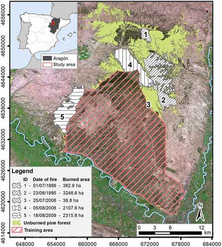
The area of interest is located in the central sector of the Ebro basin in northeastern Spain (41° 57ʹ N, 0° 57ʹ W). This area is dominated by Aleppo pine forests, and the evergreen understory is mainly composed of Quercus ilex, Quercus coccifera, Juniperus oxycedrus, Thymus vulgaris, and Rosmarinus officinalis. Part of the study area (see Figure 1) is covered by crops and occupied by a military training area, the latter of which has been excluded from the analysis. This sector of the Iberian Peninsula constitutes the northernmost semiarid region in Europe. The climate is Mediterranean with continental features (Cuadrat, Saz, and Vicente-Serrano 2007). The geomorphology of the area consists of structural platforms of Miocene carbonate and marl sediments (IGME 1995). It has a rough topography with a mean slope steepness ranging from 12 to 18º.

Figure 1 shows the extension of the forests altered by five wildfires occurring between 1986 and 2009. The burned forest, excluding the military training area, totals 8,075 ha and the unburned area 12,047 ha. More recent fires (2006–2009) underwent a post-fire intervention based on crushing burned wood and creating log erosion barriers to control erosion and seed loss (Miranda and Echevarría 2015).

Figure 1. Location of the fires and the unburned area. High spatial resolution orthophotography from PNOA Spatial Data Infrastructure (SDI) is included as backdrop.

ALS data source and pre-processing

ALS data were provided by the Geographical Institute of Aragón (IGEAR) and collected by the Spanish National Plan for Aerial Orthophotography (PNOA) between September and November 2016. The dataset was captured using a small-footprint discrete-return airborne sensor (Leica ALS80), operating at 1.064 μm wavelength and ±28 scan angle degrees from nadir. The resulting point density of the study area ranged from 1.1 to 2.0 point/m², with a vertical accuracy of ±0.1 m and a horizontal accuracy of ≤0.3 m. Data were delivered in 2 × 2 km tiles of raw data points, in LAS binary file format (v. 1.2), with up to four returns recorded per pulse.

ALS tiles were classified using the multiscale curvature classification algorithm (MCC) (Evans and Hudak 2007), implemented in the MCC 2.1 command-line tool, which was specifically developed to process discrete-return ALS data in forested environments, and is considered suitable for the study area in accordance with Montealegre, Lamelas, and de la Riva (2015a). The Point-TIN-Raster interpolation method (ArcGIS v. 10.5) was applied to the classified ground points to generate a Digital Elevation Model (DEM) with a 1 m spatial resolution in accordance with Montealegre, Lamelas, and Riva (2015b). The structural diversity of vegetation was analyzed using three types of ALS metrics: i) structural diversity indices; ii) vertical structure-related metrics; and iii) horizontal continuity metrics. These metrics were derived directly from the laser returns in accordance with Bottalico et al. (2017). Topographic metrics were also obtained from ALS data to characterize the topography of the study area.

Structural diversity indices

The LiDAR Height Diversity Index (LHDI) and the LiDAR Height Evenness Index (LHEI) were calculated in accordance with Listopad et al. (2015) (Equations 1 and 2).

(1) $LHDI=-\sum \left[\left(p_h\right)\times ln\left(p_h\right)\right]$(1)

(2) $LHEI=\frac{LHDI}{ln\left(p_h\right)}$(2)

where p is the proportion of returns at a defined height interval (h). In order to calculate the proportion of returns required by these indices, the command “DensityMetrics” (FUSION v. 3.60, McGaughey 2014) was applied. This command provides a series of raster layers where each cell contains the total number of returns for a specific range of height above ground. The metrics were computed with 10, 15, and 20 m pixel sizes to assess which spatial resolution had the best accuracies. A minimum pixel size value of 10 m was established in order to gather a sufficient number of laser returns to derive the ALS metrics. The indices were also computed at 0.5, 0.3 and 0.15 m height intervals to ascertain which vertical resolution best reflected the diversity.

Vertical structure-related metrics

A suite of statistical metrics related to the vertical height distribution of returns, commonly used as independent metrics in forestry applications, was generated using the “GridMetrics” command in FUSION 3.60 (McGaughey 2014). These metrics were also computed at 10, 15, and 20 m spatial resolutions. The height 99^th percentile (H_P99) (Equation 3) (Magnussen and Boudewyn 1998), mean height (H_mean) (Equation 4), standard deviation (H_sd) (Equation 5), kurtosis (H_kurtosis) (Equation 6), skewness (H_skewness) (Equation 7) and the canopy relief ratio (CRR) (Equation 8) (Parker and Russ 2004) were calculated.

$\left(N-1\right)P=I+d\left\{\begin{array}{c}Iistheentirepartof\left(N-1\right)P\\ distheentirepartof\left(N-1\right)P\end{array}\right\}$

where N is the number of observations and P is the percentile divided by 100.

$ifd=0thenP=x_{i+1}$

(3) $ifd>0thenP=x_{i+1}+d\left(x_{i+2}-x_{x+1}\right)$(3)

(4) $H_{\mathrm{m}\mathrm{e}\mathrm{a}\mathrm{n}}=\frac{{\sum }_{i=1}^N{x}_i}{N}$(4)

(5) ${\mathrm{H}}_{sd}=\sqrt{\frac{{\sum }_{i=1}^N{(x_i-x\mathrm{n})}^2}{N}}$(5)

(6) $H_{kurtosis}=\frac{{\sum }_{i=1}^N{(x_i-x\mathrm{n})}^4}{\left(N-1\right){\sigma }^4}$(6)

(7) $H_{skewness}=\frac{{\sum }_{i=1}^N{(x_i-x\mathrm{n})}^3}{\left(N-1\right){\sigma }^3}$(7)

(8) $Canopyreliefratio\left(CCR\right)=\frac{\bar{x}-x_{imin}}{x_{imax}-x_{imin}}$(8)

where i is the laser return, N is the total number of returns, x is the height value, is the mean height value, and σ is the standard deviation.

Horizontal continuity metrics

The canopy cover (CC) (Equation 9) was calculated using a 0.2 m height threshold to avoid ground returns, as the percentage of ground covered by the vertical projection of vegetation (Jennings, Brown, and Sheil 1999).

(9) $CanopyCover\left(CC\right)=\frac{{\sum }_{i=1}^N{r}_{ifirst}>0.2m}{{\sum }_{i=1}^N{r}_{ifirst}}\times 100$(9)

In addition, a standard deviation filter with a 3 × 3 kernel size was applied to the vertical structure metrics described previously, generating nine new horizontal continuity metrics (HCM): LHDI, LHEI, H_mean, H_sd, H_skewness, H_kurtosis, CC, CRR, H_p99.

Topographic metrics

A set of topographic metrics, such as Topographic position index (TPI), Aspect, Slope, and Roughness (Wilson et al. 2007), were also calculated to analyze the influence of terrain on vegetation structure.

Structural diversity analysis of wildfires on different dates

The percentage of returns from 0.5 to 2 m, from 2 to 4 m, and above 4 m was calculated for each wildfire, according to height ranges defined by the PROMETHEUS fuel model classification (Prometheus 2000). These ranges are suitable for the study area because the PROMETHEUS project was carried out in Mediterranean environments. The average values of LHDI and LHEI and the forest structural metrics were calculated to describe the differences between fires.

The burned areas under analysis were grouped to test whether the ALS metrics were able to distinguish between burned and unburned areas, areas burned in different years, and between old and more recent fires using a two-phase approach: i) a sample of a variable number of pixels was considered inside and outside of the fire perimeter, taking into account a minimum separation between samples to avoid spatial autocorrelation, which was analyzed using Moran’s I index; ii) the normality of the metric value distribution was tested using the Anderson–Darling test (Anderson and Darling 1954). The Kruskal–Wallis test (Kruskal and Wallis 1952) was applied when normality was not fulfilled.

Digital classification of burned areas

In order to map the burned areas, three digital classifications were performed to distinguish between burned and unburned areas (Classification 1); to differentiate the fire occurrence dates (Classification 2), and to distinguish between old and more recent fires (Classification 3). Furthermore, k-nearest neighbors algorithm (k-NN), support vector machine (SVM) and random forest (RF) methods were compared in each classification to select the most accurate technique.

k-NN is a non-parametric Machine Learning (ML) approach for classifying populations whose distributions are unknown (Fix and Hodges 1989). k-NN optimization and computation were carried out with the R package “caret” (Kuhn 2008). SVM is an ML algorithm created to analyze and recognize patterns. SVM constructs a set of hyperplanes in a high-dimensional space and tries to find the hyperplane that maximizes the separation between classes (Rodrigues and de la Riva 2014; Domingo et al. 2018). SVM parameters require optimization. In this sense, the kernel type was calibrated using the R package “kernlab,” and cost and gamma parameters were tuned, within the intervals 1–1000 and 0.01–1, respectively. SVM was computed with the R package “e1071” (Meyer et al. 2017). RF is an ML ensemble classifier that uses decision trees. The nodes of each decision tree are divided using the best variables selected from a random sample (Rodrigues and de la Riva 2014; Domingo et al. 2018). The ntree parameter was tuned within the interval 1–3000, and the number of selected variables, between 1 and the maximum number of variables −1, using the R packages “randomForest” (Liaw and Wiener 2002) and “caret” (Kuhn 2008).

Training and testing datasets to perform the digital classification were obtained from a random sample of pixels from raster metrics (Table 1). Prior to classification, variable selection was performed using the exhaustive subset selection method in accordance with Domingo et al. (2018), taking into consideration the most important metric of each type of variables analyzed (i.e. diversity indices, vertical structure, horizontal continuity, and topographic metrics). This selection was computed using the R package “leaps” (Lumley and Miller 2017).

Table 1. Training and test data set for digital classifications. Classification 1 stands for burned and unburned areas. Classification 2 stands for fire occurrence dates. Classification 3 stands for old and more recent fires.

Classification 1			Classification 2			Classification 3
Class	Training set	Test set	Class	Training set	Test set	Class	Training set	Test set
Unburned	1000 pixels	500 pixels	Unburned	1000 pixels	500 pixels	Unburned	1000 pixels	500 pixels
			Burned in 1986	1000 pixels	500 pixels
Burned	5000 pixels	2500 pixels	Burned in 1995	1000 pixels	500 pixels	Old fires	2000 pixels	1000 pixels
			Burned in 2006	1000 pixels	500 pixels
			Burned in 2008	1000 pixels	500 pixels	More recent fires	3000 pixels	1500 pixels
			Burned in 2009	1000 pixels	500 pixels

Digital classifications were validated using the test sample. Contingency tables and the percentage of overall success, which refers to the ratio between pixels correctly classified and the total number of pixels in the sample, were calculated. Moreover, Cohen’s Kappa coefficient (K) was computed to measure inter-rater agreement (Chuvieco 2010).

Results

Figure 2 shows the percentage of returns grouped by the PROMETHEUS strata for each wildfire and unburned area. In general, all areas have a similar percentage of returns in the shrub stratum (around 20%). In contrast, considerable differences are found between the tree and grass strata. For example, more than 40% of returns in unburned areas are located above 4 m, thus showing the predominance of the tree layer and a lower presence of grasslands (34.5%). In contrast, burned areas have higher variability. Those burned in relatively recent fires (2006–2009) are mainly covered by a grass layer (around 70%), while those burned in older fires have a moderate presence of grasslands (around 30%). In the case of tree strata, the presence of returns is low in more recent fires (approx. 10%) and higher in older ones (approx. 30%).

Table 2 shows the average values of the computed metrics for each wildfire and unburned area. The vegetation structure of unburned areas has high LHDI and LHEI values (1.83 and 0.71, respectively). Wildfires can be grouped into the oldest ones occurring in 1986 and 1995, and more recent ones occurring in 2006, 2008, and 2009. The areas where the oldest fires occurred have return distributions similar to the unburned areas, thus indicating an advanced stage of vegetation recovery. In particular, the area where the fire occurred in 1986 has a higher percentage of returns in the herbaceous layer than the area burned in 1995 does. This is also accompanied by higher LHDI and LHEI values (Table 2). There is a predominance of returns in the herbaceous and shrub layers, with low LHDI and LHEI values, in areas burned in relatively recent fires (2006, 2008, and 2009). In general, the areas burned in those fires have lower mean values of height (1.1–0.68 m), CC (22-37%) and CRR (0.34–0.39 m) compared to those burned in older fires and to unburned areas (Table 2).

Figure 2. Percentage of returns grouped by PROMETHEUS strata and date of fire occurrence.

Table 2. Mean values of ALS vertical metrics and diversity indices for the different occurrence dates and the unburned area.

		Year of the fire
ALS metric	Unburned	1986	1995	2006	2008	2009
LHDI	1.83	1.92	1.37	0.44	0.65	0.38
LHEI	0.71	0.81	0.72	0.32	0.47	0.28
Hmean(m)	3.34	2.57	1.67	1.10	0.87	0.68
Hsd (m)	1.94	1.45	0.82	0.58	0.49	0.40
Hskewness (m)	0.16	0.00	0.26	0.49	0.77	0.86
Hkurtosis (m)	2.75	2.40	2.09	2.86	3.45	3.44
CC (%)	71.24	81.34	64.60	22.16	37.33	24.87
CRR	0.44	0.45	0.43	0.39	35	0.34
HP99 (m)	6.68	5.24	3.29	2.07	1.99	1.56

As shown in Table 3, the results of the Kruskal–Wallis test indicate that nearly all computed metrics have statistically significant differences when considering the three different classifications, i.e. burned and unburned areas (Classification 1), fire occurrence dates (Classification 2), and old and more recent fires (Classification 3). The general tendency is similar, regardless of the pixel size and height interval for computing the diversity indices. Furthermore, there are no significant differences in the topographic metrics apart from roughness and slope in classifications 2 (fire occurrence dates) and 3 (old and more recent fires) (Table 3).

Table 3. Chi-square values for each classification (Class.), spatial resolution (10, 15, 20 m), and ALS metric. Values with non-asymptotic significance, p-value > 0.05 (^ns). Class. 1 stands for burned and unburned areas. Class. 2 stands for fire occurrence dates. Class. 3 stands for old and more recent fires. (HCM) stands for horizontal continuity metrics.

	10 m			15 m			20 m
Metric	Class. 1	Class. 2	Class. 3	Class. 1	Class. 2	Class. 3	Class. 1	Class. 2	Class. 3
Aspect	1,24^ns	3.53^ns	2.83^ns	0.80^ns	2.56^ns	1.42^ns	0.57^ns	2.43^ns	1.95^ns
CRR	14,60	72.5	71.06	24.87	98.74	94.86	41.26	122.96	120.25
CRR (HCM)	35.22	59.23	55.9	15.76	32.90	30.65	7.02	37.41	33.75
FCC	69.25	146.16	138.56	69.68	150.28	141.96	82.15	162.05	153.90
FCC (HCM)	21.67	47.34	37.96	27.36	46.43	40.16	31.28	44.02	39.44
Hkurtosis	59.08	98.95	95.83	67.56	127.68	118.17	90.49	154.47	147.88
Hkurtosis (HCM)	9.04	56.79	53.54	24.88	81.18	77.26	37.29	96.23	90.20
Hmean	178.91	234.08	223.58	200.58	253.70	244.71	210.46	263.47	255.11
Hmean (HCM)	219.22	25.39	246.05	184.22	212.74	209.96	169.75	201.96	198.10
Hp99	238.65	271.66	261.73	263.07	291.77	284.56	266.74	292.16	285.00
Hp99 (HCM)	109.68	115.82	113.32	71.28	77.99	72.29	68.84	77.98	69.11
Hsd	232.65	269.92	259.18	259.26	292.94	284.92	267.62	299.77	291.78
Hsd (HCM)	172.01	182.48	179	147.58	158.14	153.91	141.60	155.11	148.40
Hskewness	12.96	82.30	80.24	19.10	101.02	97.07	32.37	125.92	123.54
Hskewness (HCM)	2.79^ns	11.55	8.74	0.27^ns	14.34^ns	12.89	5.91	20.71	16.88
LHDI and LHEI 0.15	217.31	263.08	255.15	242.02	287.23	279.00	256.66	301.91	294.28
LHDI and LHEI0.15 (HCM)	15.77	52.28	45.89	26.86	54.93	50.27	24.17	51.88	45.43
LHDI and LHEI 0.3	229.53	268.43	260.73	248.55	288.44	280.03	268.08	309.09	300.62
LHDI and LHEI 0.3 (HCM)	16.90	269.17	30.64	16.87	30.31	24.96	11.80	23.22	17.87
LHDI and LHEI 0.5	231.66	39.12	261.37	247.18	287.66	279.13	268.59	308.90	300.79
LHDI and LHEI 0.5 (HCM)	16.16	263.08	34.19	13.16	28.57	23.21	9.64	22.20	15.47
Roughness	0.08^ns	42.21	29.9	0.07^ns	45.09	30.29	0.15^ns	37.67	26.59

The exhaustive subset selection method selected LHDI_0.15 and H_mean (HCM) as the best metrics (Table 4) for all the classifications, regardless of the spatial resolution. H_sd was also selected for classifications 1 (burned and unburned) and 3 (old and more recent fires). H_mean was selected to differentiate the fire occurrence dates (Classification 2). None of the topographic metrics were selected by the exhaustive subset method.

Table 4. Summary of the best-selected ALS metrics in Subset Selection (exhaustive method) in all classifications.

Classification	ALS metrics
Classification 1	LHDI0.15 + Hsd + Hmean (HCM)
Classification 2	LHDI0.15 + Hmean + Hmean (HCM)
Classification 3	LHDI0.15 + Hsd + Hmean (HCM)

Table 5 shows a summary of the overall classification accuracies and K indices of each classification performed with different methods and at different spatial resolutions. In the case of Classification 1 (burned and unburned areas), the best accuracy and K index was obtained using the SVM method tuned with a gamma value of 0.1 and a cost value of 500, at 15 m spatial resolution. The map obtained for Classification 1 with this method is shown in Figure 3. The overall classification accuracy was 89.44%, obtaining a K value of 0.56. Burned areas achieved the highest classification accuracy from the two defined classes (Table 6), with an omission error of 8.12%. Other classification methods and resolutions had slightly lower overall accuracy, ranging from 89.44% to 88.01%, and lower values of agreement (K = 0.56–0.48) (Table 5).

Figure 3. Classification 1 map using SVM (a) and, reference burned surface (b). A shaded relief surface is used as backdrop.

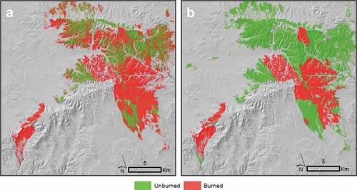
Table 5. Summary of overall classification accuracy (Acc.) and K index of each Classification performed at different spatial resolutions.

		Classification 1		Classification 2		Classification 3
Spatial resolution	Method	Acc.	K	Acc.	K	Acc.	K
10	SVM	88.72	0.54	65.60	0.59	74.73	0.57
	RF	88.79	0.55	64.20	0.57	73.45	0.54
	KNN	88.01	0.50	62.03	0.54	60.17	0.27
15	SVM	89.44	0.56	66.67	0.60	72.99	0.54
	RF	89.20	0.55	66.41	0.60	74.12	0.55
	KNN	88.44	0.50	63.50	0.56	59.83	0.26
20	SVM	89.44	0.54	65.94	0.59	75.49	0.57
	RF	88.40	0.49	67.79	0.61	75.42	0.57
	KNN	88.17	0.48	62.07	0.54	61.29	0.29

Table 6. Accuracy assessment (confusion matrix, omission and commission errors, and K index) for Classification 1 using the SVM method at 15 m resolution.

Reference data
Classification data (number of pixels)	Unburned	Burned	Total	Omission error (%)
Unburned	226	87	313	27,80%
Burned	198	2240	2438	8.12%
Total	424	2327
Commission error (%)	53.30%	3.74%
Overall classification accuracy = 89.44%; K: 0.56.

The RF method with a gamma value of 500 ntree and mtry value of 2, and at 20 m spatial resolution, was the best method for performing Classification 2 (fire occurrence dates), which considers the year of each wildfire since 1986 and the unburned area (Table 5). This classification had a moderate-high accuracy with a value of 67.79% and an overall K value of 0.61. The area burned in 2008 had the lowest classification accuracy from the six classes (Table 7), with an omission error of 46.81%. Slightly lower accuracy values were obtained for areas burned in 1986, 2009, and the unburned area (33.83%, 35.60%, and 38.82%, respectively). In contrast, a lower omission error prevailed for the area burned in 2006. Consequently, all fires can generally be distinguished with the same accuracy. According to the results shown in Table 7, there is confusion between the oldest fires and the unburned area. There is also confusion between the more recent fires, with the fire occurring in 2008 being the most misclassified one. The low variability of ALS metric values among near fire episodes may cause this confusion. In addition, small height variations between more recent fires were found when analyzing the standard deviation, thus leading to a strong confusion between them. The RF method allowed an old fire to be detected (red box in Figure 4), one that had not been recorded in the database. According to Tanase et al. (2011), this fire occurred in 1970, and its pixels were classified mostly as the 1986 fire. The other analyzed classification methods and resolutions had slightly lower overall accuracy variation, ranging from 62.07% to 67.79%, and moderate-high agreements (K = 0.54–0.61) (Table 5).

Figure 4. Classification 2 map using RF (a) and reference burned surface (b). A shaded relief surface is used as backdrop. Red box is the fire occurred in 1970.

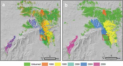
Table 7. Accuracy assessment (confusion matrix, omission and commission errors presented as percentage, and K index) for Classification 2 using the RF method at 20 m resolution.

Reference data
Classification data (number of pixels)	Unburned	1986	1995	2006	2008	2009	Total	Omission error (%)
Unburned	249	85	50	3	15	5	407	38.82%
1986	88	352	76	0	6	10	532	33.83%
1995	39	55	237	5	50	21	407	41.77%
2006	10	0	21	485	35	6	557	12.93%
2008	11	2	21	2	225	97	358	46.81%
2009	7	1	51	1	92	275	427	35.60%
Total	404	495	456	496	423	414
Commission error (%)	38.37%	28.89%	48.03%	2.22%	46.81%	33.57%
Overall classification accuracy = 67.79%; K: 0.61

The radial-basis kernel SVM with a gamma value of 0.1 and a cost value of 50, at 20 m spatial resolution, was the best method for performing Classification 3 (Table 5, Figure 5). This classification had a moderate-high accuracy with a value of 75.49% and an overall K value of 0.57. Table 8 shows the difficulty in accurately differentiating the older fires from the unburned area. This classification has slight differences in terms of overall accuracy compared with RF and SVM with radial kernel (75.42% and 75.42%, respectively), and a greater difference compared with k-NN (61.29%). The K index values range from 0.26 to 0.57 (Table 5).

Figure 5. Classification 3 using SVM (a), and reference burned surface (b). A shaded relief surface is used as backdrop.

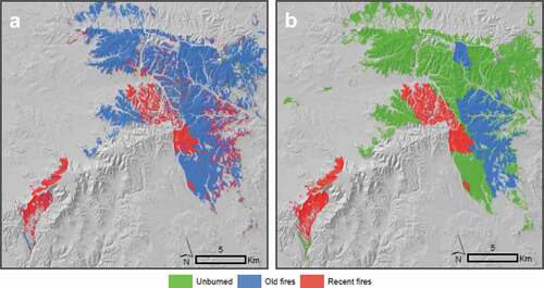
Table 8. Accuracy assessment (confusion matrix, omission and commission errors presented as percentage, and K index) for Classification 3 using the SVM method at 20 m resolution.

Reference data
Classification data (number of pixels)	Unburned	Old fires	Recent fires	Total	Omission error (%)
Unburned	22	11	11	44	50.00%
Old fires	338	799	113	1250	36.08%
Recent fires	44	142	1209	1395	13.33%
Total	404	952	1333
Commission error (%)	5.45%	83.93%	90.70%
Overall classification accuracy = 75.49%; K: 0.57

Discussion

Forest fires are significant events in the Mediterranean basin, causing partial or total destruction of the forest structure (Alexandrian, Esnault, and Calabri 1999). Post-fire Aleppo pine forest regeneration has high variability due to weather conditions, land uses, and post-dispersal seed predation (Pausas et al. 2009). Our results show that relatively recent fires (occurring in 2006, 2008, and 2009) have similar return distributions in all strata, consistent with the temporal proximity of the fire episodes. These wildfires have the lowest LHDI and LHEI values, and most of the laser returns are located in the shrub layer (70%), thus implying structural homogeneity of the vegetation. As defined in Parker and Russ (2004), lower CRR values also indicate that tree branches are located in the lower part of the trunk. As mentioned further above, it should be noted that these fires underwent a post-fire intervention (Miranda and Echevarría 2015).

The oldest fires, occurring in 1986 and 1995, have return distributions closer to the unburned area. This could be a consequence of the time that has passed since the fire. According to Rodrigues et al. (2014), that may have led to an advanced stage of recovery. Consistent with the equitable distribution of laser returns in height ranges, the LHDI and LHEI indices have high values, thus implying greater forest structural diversity compared to areas burned in relatively recent fires (Listopad et al. 2015). The increase in structural diversity is especially high, even surpassing the values of the unburned area, in the case of the area burned in the fire occurring in 1986. This area was affected by an extensive extraction of burned wood, a common practice in post-fire treatment in Spain (Castro et al. 2009). In comparison to 0.3 or 0.5 m height intervals, the generation of diversity indices (LHDI-LHEI) at a 0.15 m height interval better reflects the distribution of the forest structure due to the dense understory in Pinus halepensis forests. This distribution variability is also well reflected by the H_sd metric, in agreement with Zimble et al. (2003) and Brandtberg et al. (2003)

In terms of distinguishing between similar classes, SVM and RF had better accuracies than k-NN. Similar results were obtained by Abu Alfeilat et al. (2019). Given the proximity of dates between some fires, it was difficult to accurately classify them individually. However, the moderate accuracy results obtained and the fact that an unrecorded fire occurring in 1970 was found together reinforce the validity of the method in Classification 2. Despite the difficulty in distinguishing between the unburned area and the old fires (83.93% commission error in the old fire class), there were significant differences in the Kruskal–Wallis test, given the mature stage of these burned forests. Previous studies have analyzed post-fire regeneration using Tasseled Cap transformation or vegetation index time series (Vicente-Serrano, Pérez-Cabello, and Lasanta 2011; Fernandez-Manso, Quintano, and Roberts 2016; Martínez et al. 2017), and they too had problems differentiating older disturbances from mature forests.

Gómez et al. (2019) reviewed the recent publications devoted to forest studies employing remote sensing in Spain, and they concluded that, based on recovery values calculated using optical data, the pre-fire state was reached somewhere between 7 and 20 years after the time of the disturbance because regrowth processes were affected by a complex mosaic of bare soil, shrubs, and herbaceous species (Vicente-Serrano, Pérez-Cabello, and Lasanta 2011). The main advantage of active sensors over multispectral instruments is their ability to capture three-dimensional information of the vegetation structure (Montealegre et al. 2016; Chen et al. 2018; Fernandez-Carrillo et al. 2018). Montealegre et al. (2016, 2017) and Domingo et al. (2017, 2019) used a PNOA ALS dataset to calculate forest-stand metrics, achieving good models for relating mean height, squared mean diameter, basal area, timber volume, and even carbon dioxide emissions of the aboveground tree biomass in case of a fire event. Synthetic Aperture Radar (SAR) data have been used for detecting wildfires by Tanase et al. (2011), who detected disturbances some 40 to 60 years after their occurrence. In this regard, our study offers results with accuracies comparable to SAR, with the ability to classify fires ~35 years after their occurrence. Although SAR sensors may be suitable for the three-dimensional characterization of forest ecosystems, and despite the fact that there have been recent advances in data processing, difficulties still arise when estimating forest structure in heterogeneous and dense forests (Hyde et al. 2006; Tanase et al. 2011). Our approach provides valuable information and reduces the time and costs involved in analyzing forest structural diversity at the landscape level. Furthermore, it is spatially transferable to other forest environments when 3D LiDAR data captured at regional scales are made available (Listopad et al. 2015).

The main limitation of the data source used in this study is that of capturing post-fire forest structure regeneration in a highly recurrent fire regime scenario. Within the context of climate change, San-Miguel-Ayanz, Moreno, and Camia (2013) have suggested that more arid conditions could increase the frequency of extreme fires, which would alter recovery capacity (González-De Vega, de Las Heras, and Moya 2018) and produce a loss of species diversity (Fernández-García et al. 2019). Fire recurrence might reduce forest vertical complexity, thus generating forested environments dominated by grasslands and shrublands, where trees do not reach their mature stage.

Conclusions

ALS datasets are becoming available to users, but applications focusing on the analysis of forest structural diversity are still limited. Our results demonstrate the feasibility of low point density ALS data to obtain structural diversity indices and a suite of metrics that enable the characterization of the Pinus halepensis forest structure, one that is recurrently affected by fires in the Mediterranean basin. The most suitable ALS-derived metrics were LHDI_0.15, H_sd, H_mean (HCM), which were used to perform digital classifications for mapping burned and unburned areas (Classification 1); to differentiate fire occurrence dates (Classification 2); and to distinguish between old and more recent fires (Classification 3). In general, the SVM classification method offered higher accuracies. RF also showed a similar performance, although it was slightly better at differentiating between occurrence dates. In contrast, k-NN provided the least accurate results. The proposed methodology has enabled burned areas to be detected at least 35 years after their occurrence and is therefore useful for assisting forest management at the landscape scale.

Disclosure Statement

No potential conflict of interest was reported by the authors.

Additional information

Funding

This work was supported by the Instituto de Investigación en Ciencias Ambientales de Aragón (IUCA) under scholarship [University of Zaragoza PEX-16-076], and by the research grant program Ajuts UdL, Jade Plus i Fundació Bancària La Caixa [Agreement 79/2018 of the Governing Council of the University of Lleida]. This research article has received a grant for its linguistic revision from the Language Institute of the University of Lleida (2020 call).

References

- Abu Alfeilat, H. A., A. B. A. Hassanat, O. Lasassmeh, A. S. Tarawneh, M. B. Alhasanat, H. S. Eyal Salman, and V. B. S. Prasath. 2019. “Effects of Distance Measure Choice on K-Nearest Neighbor Classifier Performance: A Review.” Big Data 7: 221–248. doi:10.1089/big.2018.0175.
- Aguilar, F. J., J. P. Mills, J. Delgado, M. A. Aguilar, J. G. Negreiros, and J. L. Pérez. 2010. “Modelling Vertical Error in LiDAR-Derived Digital Elevation Models.” ISPRS Journal of Photogrammetry and Remote Sensing 65: 103–110. doi:10.1016/j.isprsjprs.2009.09.003.
- Alexandrian, D., F. Esnault, and G. Calabri. 1999. “Forest Fires in the Mediterranean Area.” Unasylva (FAO).
- Anderson, T. W., and D. A. Darling. 1954. “A Test of Goodness of Fit.” Journal of the American Statistical Association 49: 765–769. doi:10.1080/01621459.1954.10501232.
- Bottalico, F., G. Chirici, R. Giannini, S. Mele, M. Mura, M. Puxeddu, R. E. McRoberts, R. Valbuena, and D. Travaglini. 2017. “Modeling Mediterranean Forest Structure Using Airborne Laser Scanning Data.” International Journal of Applied Earth Observation and Geoinformation 57: 145–153. Elsevier. doi:10.1016/j.jag.2016.12.013.
- Brandtberg, T., T. A. Warner, R. E. Landenberger, and J. B. McGraw. 2003. “Detection and Analysis of Individual Leaf-off Tree Crowns in Small Footprint, High Sampling Density Lidar Data from the Eastern Deciduous Forest in North America.” Remote Sensing of Environment 85: 290–303. doi:10.1016/S0034-4257(03)00008-7.
- Castro, J., R. Navarro, J. R. Guzmán, R. Zamora, and S. Bautista. 2009. “¿Es Conveniente Retirar La Madera Quemada Tras Un Incendio Forestal?” Quercus 281: 34–41.
- Chen, W., H. Jiang, K. Moriya, T. Sakai, and C. Cao. 2018. “Monitoring of Post-Fire Forest Regeneration under Different Restoration Treatments Based on ALOS/PALSAR Data.” New Forests 49 (1): 105–121. doi:10.1007/s11056-017-9608-2.
- Chuvieco, E. 2010. Teledetección Ambiental. La Observación de La Tierra Desde El Espacio. Barcelona: Ariel Ciencia.
- Cochrane, M. A., and M. D. Schulze. 1999. “Fire as a Recurrent Event in Tropical Forests of the Eastern Amazon: Effects on Forest Structure, Biomass, and Species Composition.” Biotropica 31 (1): 2–16. Wiley Online Library.
- Cuadrat, J. M., M. A. Saz, and S. M. Vicente-Serrano. 2007. “Atlas Climático de Aragón.” Gobierno de Aragón.
- Debouk, H., R. Riera-Tatché, and C. Vega-Garcia. 2013. “Assessing Post-Fire Regeneration in a Mediterranean Mixed Forest Using LiDAR Data and Artificial Neural Networks.” Photogrammetric Engineering & Remote Sensing 79 (12): 1121–1130. American Society for Photogrammetry and Remote Sensing. doi:10.14358/PERS.79.12.1121.
- Domingo, D., A. L. Montealegre, M. T. Lamelas, A. García-Martín, J. de la Riva, F. Rodríguez, and R. Alonso. 2019. “Quantifying Forest Residual Biomass in Pinus Halepensis Miller Stands Using Airborne Laser Scanning Data.” GIScience and Remote Sensing 56 (8): 1210–1232. Taylor & Francis. doi:10.1080/15481603.2019.1641653.
- Domingo, D., M. T. Lamelas, A. L. Montealegre, A. García-Martín, and J. de la Riva. 2018. “Estimation of Total Biomass in Aleppo Pine Forest Stands Applying Parametric and Nonparametric Methods to Low-Density Airborne Laser Scanning Data.” Forests 9 (4): 158. Multidisciplinary Digital Publishing Institute. doi:10.3390/f9040158.
- Domingo, D., M. T. Lamelas, A. L. Montealegre, and J. de la Riva. 2017. “Comparison of Regression Models to Estimate Biomass Losses and CO2 Emissions Using Low-Density Airborne Laser Scanning Data in a Burnt Aleppo Pine Forest.” European Journal of Remote Sensing 50 (1): 384–396. doi:10.1080/22797254.2017.1336067.
- Dubayah, R. O., and J. B. Drake. 2000. “Lidar Remote Sensing for Forestry.” Journal of Forestry 98 (6): 44–46. Oxford University Press.
- Evans, J. S., and A. T. Hudak. 2007. “A Multiscale Curvature Algorithm for Classifying Discrete Return LiDAR in Forested Environments.” IEEE Transactions on Geoscience and Remote Sensing 45 (4): 1029–1038. doi:10.1109/TGRS.2006.890412.
- Fernandez-Carrillo, A., L. McCaw, M. A. Belenguer-Plomer, and M. A. Tanase. 2018. “L-Band SAR Sensitivity to Prescribed Burning Effects in Eucalypt Forests of Western Australia.” Proc. SPIE 10788, Active and Passive Microwave Remote Sensing for Environmental Monitoring II, 107880U (9 October 2018). doi:10.1117/12.2325669
- Fernández-García, V., P. Z. Fulé, E. Marcos, and L. Calvo. 2019. “The Role of Fire Frequency and Severity on the Regeneration of Mediterranean Serotinous Pines under Different Environmental Conditions.” Forest Ecology and Management 444: 59–68. doi:10.1016/j.foreco.2019.04.040.
- Fernandez-Manso, A., C. Quintano, and D. A. Roberts. 2016. “Burn Severity Influence on Post-Fire Vegetation Cover Resilience from Landsat MESMA Fraction Images Time Series in Mediterranean Forest Ecosystems.” Remote Sensing of Environment 184 (October): 112–123. Elsevier. doi:10.1016/J.RSE.2016.06.015.
- Fix, E., and J. L. Hodges. 1989. “Discriminatory Analysis. Nonparametric Discrimination: Consistency Properties.” International Statistical Review 57: 238–247. doi:10.2307/1403797.
- García, M., D. Riaño, E. Chuvieco, J. Salas, and F. Danson. 2011. “Multispectral and LiDAR Data Fusion for Fuel Type Mapping Using Support Vector Machine and Decision Rules.” Remote Sensing of Environment 115 (6): 1369–1379. Elsevier. doi:10.1016/j.rse.2011.01.017.
- Gómez, C., P. Alejandro, T. Hermosilla, F. Montes, C. Pascual, L. A. Ruiz, F. Álvarez-Taboada, M. A. Tanase, and R. Valbuena. 2019. “Remote Sensing for the Spanish Forests in the 21st Century: A Review of Advances, Needs, and Opportunities.” Forest Systems 28: eR001. doi:10.5424/fs/2019281-14221.
- Gonçalves, A. C., and A. Sousa. 2017 The fire in the Mediterranean region: a case study of forest fires in Portugal. Mediterranean Identities-Environment, Society, Culture; Fuerst-Bielis, B., Ed, 305–335.
- González-De Vega, S., J. de Las Heras, and D. Moya. 2018. “Post-Fire Regeneration and Diversity Response to Burn Severity in Pinus Halepensis Mill. Forests.” Forests 9 (6): 299. Multidisciplinary Digital Publishing Institute. doi:10.3390/f9060299.
- González-De Vega, S., J. De Las Heras, and D. Moya. 2016. “Resilience of Mediterranean Terrestrial Ecosystems and Fire Severity in Semiarid Areas: Responses of Aleppo Pine Forests in the Short, Mid and Long Term.” Science of the Total Environment 573: 1171–1177. doi:10.1016/j.scitotenv.2016.03.115.
- Goubitz, S., R. Nathan, R. Roitemberg, A. Shmida, and G. Ne’eman. 2004. “Canopy Seed Bank Structure in Relation To: Fire, Tree Size and Density.” Plant Ecology 173 (2): 191–201. Springer. doi:10.1023/B:VEGE.0000029324.40801.74.
- Hamraz, H., M. A. Contreras, and J. Zhang. 2017. “Forest Understory Trees Can Be Segmented Accurately within Sufficiently Dense Airborne Laser Scanning Point Clouds.” Scientific Reports 7. doi:10.1038/s41598-017-07200-0.
- Hansen, A. J., L. B. Phillips, R. Dubayah, S. Goetz, and M. Hofton. 2014. “Regional-Scale Application of Lidar: Variation in Forest Canopy Structure across the Southeastern US.” Forest Ecology and Management 329: 214–226. Elsevier. doi:10.1016/j.foreco.2014.06.009.
- Hyde, P., R. Dubayah, W. Walker, J. B. Blair, M. Hofton, and C. Hunsaker. 2006. “Mapping Forest Structure for Wildlife Habitat Analysis Using Multi-Sensor (Lidar, SAR/ InSAR,ETM+, Quickbird) Synergy.” Remote Sensing of Environment 102 (1–2): 63–73. Elsevier. doi:10.1016/j.rse.2006.01.021.
- IGME. 1995. “Mapa Geológico de España a Escala 1:50.000.”
- Jennings, S. B., N. D. Brown, and D. Sheil. 1999. “Assessing Forest Canopies and Understorey Illumination: Canopy Closure, Canopy Cover and Other Measures.” Forestry: an International Journal of Forest Research 72 (1): 59–74. Oxford University Press. doi:10.1093/forestry/72.1.59.
- Jiménez-Ruano, A., M. Rodrigues, and J. de la Riva. 2017. “Exploring Spatial–Temporal Dynamics of Fire Regime Features in Mainland Spain.” Natural Hazards and Earth System Sciences 17: 1697–1711. doi:10.5194/nhess-17-1697-2017.
- Kane, V. R., J. A. Lutz, S. L. Roberts, D. F. Smith, R. J. McGaughey, N. A. Povak, and M. L. Brooks. 2013. “Landscape-Scale Effects of Fire Severity on Mixed-Conifer and Red Fir Forest Structure in Yosemite National Park.” Forest Ecology and Management 287: 17–31. Elsevier. doi:10.1016/j.foreco.2012.08.044.
- Kelly, M., and S. Di Tommaso. 2015. “Mapping Forests with Lidar Provides Flexible, Accurate Data with Many Uses.” California Agriculture 69 (1): 14–20. University of California, Agriculture and Natural Resources. doi:10.3733/ca.v069n01p14.
- Kimmins, J. P. 1997. “Biodiversity and Its Relationship to Ecosystem Health and Integrity.” The Forestry Chronicle 73 (2): 229–232. NRC Research Press Ottawa, Canada. doi:10.5558/tfc73229-2.
- Kruskal, W. H., and W. A. Wallis. 1952. “Use of Ranks in One-Criterion Variance Analysis.” Journal of the American Statistical Association 47 (260): 583–621. doi:10.1080/01621459.1952.10483441.
- Kuhn, M. 2008. “Building Predictive Models in R Using the Caret Package.” Journal of Statistical Software 28 (5): 1–26. doi:10.18637/jss.v028.i05.
- Lamelas, M. T., D. Riaño, and S. Ustin. 2019. “A LiDAR Signature Library Simulated from 3-Dimensional Discrete Anisotropic Radiative Transfer (DART) Model to Classify Fuel Types Using Spectral Matching Algorithms.” GIScience and Remote Sensing 56 (7): 988–1023. Taylor & Francis. doi:10.1080/15481603.2019.1601805.
- Lefsky, M. A., W. B. Cohen, G. G. Parker, and D. J. Harding. 2002. “Lidar Remote Sensing for Ecosystem Studies.” BioScience 52 (1): 19–30. doi:10.1641/0006-3568(2002)052[0019:LRSFES]2.0.CO;2.
- Liaw, A., and M. Wiener. 2002. “Classification and Regression by RandomForest.” R News 2 (3): 18–22.
- Lim, K., P. Treitz, M. A. Wulder, B. St-Onge, and M. Flood. 2003. “LiDAR Remote Sensing of Forest Structure.” Progress in Physical Geography 27 (1): 88–106. doi:10.1191/0309133303pp360ra.
- Listopad, C. M. C. S., R. E. Masters, J. Drake, J. Weishampel, and C. Branquinho. 2015. “Structural Diversity Indices Based on Airborne LiDAR as Ecological Indicators for Managing Highly Dynamic Landscapes.” Ecological Indicators 57: 268–279. Elsevier. doi:10.1016/j.ecolind.2015.04.017.
- Liu, X. 2008. “Airborne LiDAR for DEM Generation: Some Critical Issues.” Progress in Physical Geography 32 (1): 31–49. Sage Publications Sage UK: London, England. doi:10.1177/0309133308089496.
- Lumley, T., and A. Miller. 2017. “Leaps: Regression Subset Selection.” https://CRAN.Rproject.org/package=leaps
- Magnussen, S., and P. Boudewyn. 1998. “Derivations of Stand Heights from Airborne Laser Scanner Data with Canopy-Based Quantile Estimators.” Canadian Journal of Forest Research 28 (7): 1016–1031. NRC Research Press. doi:10.1139/x98-078.
- Manzanera, Jose A., A. García-Abril, C. Pascual, R. Tejera, S. Martín-Fernández, T. Tokola, and R. Valbuena. 2016. “Fusion of Airborne Lidar and Multispectral Sensors Reveals Synergic Capabilities in Forest Structure Characterization.” GIscience and Remote Sensing 53 (6): 723–38. doi: 10.1080/15481603.2016.1231605.
- Martín-Alcón, S., C. Ll, M. De Cáceres, L. Guitart, M. Cabré, A. Just, and J. R. González-Olabarría. 2015. “Combining Aerial LiDAR and Multispectral Imagery to Assess Postfire Regeneration Types in a Mediterranean Forest.” Canadian Journal of Forest Research 45: 856–866. doi:10.1139/cjfr-2014-0430.
- Martínez, S., E. Chuvieco, I. Aguado, and J. Salas. 2017. “Severidad y Regeneración En Grandes Incendios Forestales: Análisis a Partir de Series Temporales de Imágenes Landsat.” Revista de Teledeteccion 2017 (49 Special Issue): 17–32. Universitat Politecnica de Valencia. doi:10.4995/raet.2017.7182.
- McElhinny, C., P. Gibbons, C. Brack, and J. Bauhus. 2005. “Forest and Woodland Stand Structural Complexity: Its Definition and Measurement.” Forest Ecology and Management 218 (1–3): 1–24. Elsevier. doi:10.1016/j.foreco.2005.08.034.
- McGaughey, R. J. 2014. “FUSION/LDV: Software for LIDAR Data Analysis and Visualization. March 2014–FUSION, Version 3.42.” United States Department of Agriculture Forest Service Pacific Northwest Research Station.
- Medail, F., and P. Quezel. 1999. “Biodiversity Hotspots in the Mediterranean Basin: Setting Global Conservation Priorities.” Conservation Biology 13: 1510–1513. doi:10.1046/j.1523-1739.1999.98467.x.
- Meyer, D., E. Dimitriadou, K. Hornik, A. Weingessel, and F. Leisch. 2017. “E1071: Misc Functions of the Department of Statistics, Probability Theory Group (Formerly: E1071), TU Wien. R Package Version 1.6-8.”
- Miranda, J., and M. T. Echevarría. 2015. “Aproximación, a Partir de Un Modelo de Vulnerabilidad, a Técnicas de Rehabilitación En Zonas Afectadas Por Incendios Forestales.” In Análisis Espacial y Representación Geográfica: Innovación y Aplicación, edited by J. de la Riva, P. Ibarra, R. Montorio, and M. Rodrigues, 691–697, University of Zaragoza, Zaragoza.
- Montealegre, A., M. Lamelas, and J. Riva. 2015b. “Interpolation Routines Assessment in ALS-Derived Digital Elevation Models for Forestry Applications.” Remote Sensing 7 (7): 8631–8654. Multidisciplinary Digital Publishing Institute. doi:10.3390/rs70708631.
- Montealegre, A. L., M. T. Lamelas, A. García-Martín, J. de la Riva, and E. Francisco. 2017. “Using Low-Density Discrete Airborne Laser Scanning Data to Assess the Potential Carbon Dioxide Emission in case of a Fire Event in a Mediterranean Pine Forest.” GIScience and Remote Sensing 54 (5): 721–740. Taylor & Francis. doi:10.1080/15481603.2017.1320863.
- Montealegre, A. L., M. T. Lamelas, and J. de la Riva. 2015a. “A Comparison of Open-Source LiDAR Filtering Algorithms in A Mediterranean Forest Environment.” IEEE Journal of Selected Topics in Applied Earth Observations and Remote Sensing 8 (8): 4072–4085. doi:10.1109/JSTARS.2015.2436974.
- Montealegre, A. L., M. T. Lamelas, J. de la Riva, A. García-Martín, and F. Escribano. 2016. “Use of Low Point Density ALS Data to Estimate Stand-Level Structural Variables in Mediterranean Aleppo Pine Forest.” Forestry 89 (4): 373–382. doi:10.1093/forestry/cpw008.
- Parker, G. G., and M. E. Russ. 2004. “The Canopy Surface and Stand Development: Assessing Forest Canopy Structure and Complexity with near-Surface Altimetry.” Forest Ecology and Management 189 (1–3): 307–315. Elsevier. doi:10.1016/j.foreco.2003.09.001.
- Pausas, J. 2004. “Changes in Fire and Climate in the Eastern Iberian Peninsula (Mediterranean Basin).” Climatic Change 63 (3): 337–350. Springer. doi:10.1023/B:CLIM.0000018508.94901.9c.
- Pausas, J., J. Llovet, A. Rodrigo, and R. Vallejo. 2009. “Are Wildfires a Disaster in the Mediterranean Basin?–A Review.” International Journal of Wildland Fire 17 (6): 713–723. CSIRO. doi:10.1071/WF07151.
- Pielou, E. C. 1975. Ecological Diversity. Wiley.New York, pp 165.
- Prometheus, S. V. 2000. “Management Techniques for Optimization of Suppression and Minimization of Wildfire Effects.” System Validation. European Commission–Contract Number ENV4-CT98-0716.
- Rodrigues, M., I. Paloma, M. T. Echeverría, F. Pérez-Cabello, and J. de la Riva. 2014. “A Method for Regional-Scale Assessment of Vegetation Recovery Time after High-Severity Wildfires: Case Study of Spain.” Progress in Physical Geography 38 (5): 556–575. doi:10.1177/0309133314542956.
- Rodrigues, M., and J. de la Riva. 2014. “An Insight into Machine-Learning Algorithms to Model Human-Caused Wildfire Occurrence.” Environmental Modelling & Software 57: 192–201. Elsevier. doi:10.1016/j.envsoft.2014.03.003.
- Rodrigues, M., J. San-Miguel-Ayanz, S. Oliveira, F. Moreira, and A. Camia. 2013. “An Insight into Spatial-Temporal Trends of Fire Ignitions and Burned Areas in the European Mediterranean Countries.” Journal of Earth Science and Engineering 3 (7): 497. David Publishing Company, Inc.
- San-Miguel-Ayanz, J., J. M. Moreno, and A. Camia. 2013. “Analysis of Large Fires in European Mediterranean Landscapes: Lessons Learned and Perspectives.” Forest Ecology and Management 294: 11–22. doi:10.1016/j.foreco.2012.10.050.
- Shannon, C. E., and W. Weaver. 1949. The Mathematical Theory of Communication. Urbana, IL: University of illinois Press IL.
- Staudhammer, C. L., and V. M. LeMay. 2001. “Introduction and Evaluation of Possible Indices of Stand Structural Diversity.” Canadian Journal of Forest Research 31 (7): 1105–1115. NRC Research Press. doi:10.1139/x01-033.
- Su, J., and E. Bork. 2006. “Influence of Vegetation, Slope, and Lidar Sampling Angle on DEM Accuracy.” Photogrammetric Engineering & Remote Sensing 72 (11): 1265–1274. American Society for Photogrammetry and Remote Sensing. doi:10.14358/PERS.72.11.1265.
- Tanase, M. A., J. De la riva, M. Santoro, F. Pérez-Cabello, and E. Kasischke. 2011. “Sensitivity of SAR Data to Post-Fire Forest Regrowth in Mediterranean and Boreal Forests.” Remote Sensing of Environment 115 (8): 2075–2085. Elsevier. doi:10.1016/j.rse.2011.04.009.
- Teobaldelli, M., F. Cona, L. Saulino, A. Migliozzi, G. D’Urso, G. Langella, P. Manna, and A. Saracino. 2017. “Detection of Diversity and Stand Parameters in Mediterranean Forests Using Leaf-off Discrete Return LiDAR Data.” Remote Sensing of Environment 192: 126–138. Elsevier. doi:10.1016/j.rse.2017.02.008.
- Vicente-Serrano, S. M., F. Pérez-Cabello, and T. Lasanta. 2011. “Pinus Halepensis Regeneration after a Wildfire in a Semiarid Environment: Assessment Using Multitemporal Landsat Images.” International Journal of Wildland Fire 20: 195. doi:10.1071/WF08203.
- Wilson, M. F. J., B. O’Connell, C. Brown, J. C. Guinan, and A. J. Grehan. 2007. “Multiscale Terrain Analysis of Multibeam Bathymetry Data for Habitat Mapping on the Continental Slope.” Marine Geodesy 30: 3–35. doi:10.1080/01490410701295962.
- Wulder, M. A., J. C. White, R. F. Nelson, E. Næsset, H. Ole, N. C. Coops, T. Hilker, C. W. Bater, and T. Gobakken. 2012. “Lidar Sampling for Large-Area Forest Characterization: A Review.” Remote Sensing of Environment 121: 196–209. Elsevier B.V.. doi:10.1016/j.rse.2012.02.001.
- Zimble, D. A., D. L. Evans, G. C. Carlson, R. C. Parker, S. C. Grado, and P. D. Gerard. 2003. “Characterizing Vertical Forest Structure Using Small-Footprint Airborne LiDAR.” Remote Sensing of Environment 87 (2–3): 171–182. Elsevier. doi:10.1016/S0034-4257(03)00139-1.