Surface roughness signatures of summer arctic snow-covered sea ice in X-band dual-polarimetric SAR

ABSTRACT

Surface roughness of sea ice is primary information for understanding sea ice dynamics and air–ice–ocean interactions. Synthetic aperture radar (SAR) is a powerful tool for investigating sea ice surface roughness owing to the high sensitivity of its signal to surface structures. In this study, we explored the surface roughness signatures of the summer Arctic snow-covered first-year sea ice in X-band dual-polarimetric SAR in terms of the root mean square (RMS) height. Two ice campaigns were conducted for the first-year sea ice with dry snow cover in the marginal ice zone of the Chukchi Sea in August 2017 and August 2018, from which high-resolution (4 cm) digital surface models (DSMs) of the sea ice were derived with the help of a terrestrial laser scanner to obtain the in situ RMS height. X-band dual-polarimetric (HH and VV) SAR data (3 m spatial resolution) were obtained for the 2017 campaign, at a high incidence angle (49.5°) of TerraSAR-X, and for the 2018 campaign, at a mid-incidence angle (36.1°) of TanDEM-X 1–2 days after the acquisition of the DSMs. The sea ice drifted during the time between the SAR and DSM acquisitions. As it is difficult to directly co-register the DSM to SAR owing to the difference in spatial resolution, the two datasets were geometrically matched using unmanned aerial vehicle (4 cm resolution) and helicopter-borne (30 cm resolution) photographs acquired as part of the ice campaigns. A total of five dual-polarimetric SAR features―backscattering coefficients at HH and VV polarizations, co-polarization ratio, co-polarization phase difference, and co-polarization correlation coefficient ―were computed from the dual-polarimetric SAR data and compared to the RMS height of the sea ice, which showed macroscale surface roughness. All the SAR features obtained at the high incidence angle were statistically weakly correlated with the RMS height of the sea ice, possibly influenced by the low backscattering close to the noise level that is attributed to the high incidence angle. The SAR features at the mid-incidence angle showed a statistically significant correlation with the RMS height of the sea ice, with Spearman’s correlation coefficient being higher than 0.7, except for the co-polarization ratio. Among the intensity-based and polarimetry-based SAR features, HH-polarized backscattering and co-polarization phase difference were analyzed to be the most sensitive to the macroscale RMS height of the sea ice. Our results show that the X-band dual-polarimetric SAR at mid-incidence angle exhibits potential for estimation of the macroscale surface roughness of the first-year sea ice with dry snow cover in summer.

KEYWORDS:

• Sea ice surface roughness
• root mean square (RMS) height
• snow-covered first-year sea ice
• synthetic aperture radar (SAR)
• x-band dual polarimetry

1. Introduction

Surface roughness is a key indicator of the type and thickness of sea ice (Scharien and Yackel 2005; Von Saldern, Haas, and Dierking 2006; Peterson, Prinsenberg, and Holladay 2008; Kim, Kim, and Hwang 2012; Fors et al. 2016a). Sea ice surface roughness also impacts ice-albedo feedback and contributes to the changes in the solar energy input to sea ice and the formation of melt ponds, which are common features of the summer Arctic sea ice surface (Eicken et al. 2004; Scharien and Yackel 2005). The surface roughness of sea ice is related to the air–ice and ice–water drag coefficients (Andreas et al. 1993; Fisher and Lytle 1998; Lu et al. 2011; Castellani et al. 2014), which are important parameters for determining the momentum balance of sea ice and improving global climate prediction models (Lüpkes et al. 2012, 2013; Castellani et al. 2018). Therefore, observing the surface roughness of sea ice is crucial for a better understanding of the dynamics of sea ice cover and its impact on global climate change.

Satellite remote sensing has been widely used in the observation of sea ice surface roughness. In optical remote sensing, surface roughness is one of the factors influencing the spectral signatures of sea ice (Nolin, Fetterer, and Scambos 2002; Nolin and Mar 2019). However, these optical images are useless on cloudy days and at night. Microwave remote sensing can observe the earth’s surface, regardless of the weather conditions and the altitude of the sun; thus, it can be more useful in investigating sea ice surface roughness than optical remote sensing. In several studies, sea ice roughness has been analyzed with passive microwave sensors owing to the fact that it impacts the properties of microwave radiation (Stroeve et al. 2006; Hong 2010; Hong and Shin 2010; Bi et al. 2013; Gupta et al. 2014; Kim et al. 2015). Although passive microwave sensors can cover the whole Arctic and Antarctica every day, their low spatial resolution (~25 km) is a limiting factor in spatially precise investigation of sea ice surface roughness.

Synthetic aperture radar (SAR), an active microwave remote sensing system, can be useful in the investigation of sea ice surface roughness because the backscattered radar signals are sensitive to surface structural characteristics. SAR can provide information regarding sea ice with a higher spatial resolution (<100 m) than passive microwave sensors and other spaceborne active microwave remote sensing sensors, such as scatterometers (a few kilometers) and radar altimeters (a few hundred meters). Spaceborne microwave scatterometers and radar altimeters also measure the radar return signals from sea ice and provide information on the ice surface characteristics (Swift 1999; Swan and Long 2012; Kurz, Galin, and Studinger 2014), but their lower spatial resolution is insufficient for an accurate investigation of surface roughness.

Current SAR satellites acquiring multi-polarization data, such as TerraSAR-X, TanDEM-X, Radarsat-2, and ALOS-2, have provided various polarimetric parameters that represent the physical properties of targets. In the field of sea ice, polarimetric SARs have been widely used for ice/water discrimination (Geldsetzer and Yackel 2009; Leigh, Wang, and Clausi 2014; Zakhvatkina et al. 2017), classification of sea ice type (Gill and Yackel 2012; Dabboor and Geldsetzer 2014; Ressel, Frost, and Lehner 2015; Fors et al. 2016a; Ressel et al. 2016), estimation of sea ice thickness (Nakamura et al. 2006, 2009; Kim, Kim, and Hwang 2012; Zhang et al. 2016), and detection of melt ponds (Scharien, Landy, and Barber 2014; Han et al. 2016; Ramjan et al. 2018). Several studies have used airborne (Wakabayashi et al. 2004; Nakamura et al. 2006) and shipborne (Gupta, Scharien, and Barber 2013) polarimetric SAR data in sea ice surface roughness investigations, but few studies have been performed based on satellite polarimetric SAR. A recent study investigated the sea ice surface roughness by using the fully polarimetric Radarsat-2 C-band SAR (Fors et al. 2016b). Most of the studies on sea ice roughness based on satellite SARs were conducted using single-polarization data (Scharien and Yackel 2005; Dierking and Busche 2006; Peterson, Prinsenberg, and Holladay 2008; Toyota et al. 2011; Liu et al. 2015). Although radar backscattering is sensitive to ice surface morphology, single-polarized signals are less efficient in investigating sea ice roughness than multi-polarized ones because they provide insufficient information about the surface structures of the ice. Moreover, most of the previous studies were conducted near the coast, and offshore sea ice was hardly investigated. This is because it is difficult to access offshore sea ice and acquire the in situ surface roughness, which is essential for validating the remote sensing-based estimation.

X-band polarimetric SAR can be more useful for the investigation of sea ice surface roughness than C- and L-band SARs because it involves shorter wavelengths and the measured radar signals reflect more ice surface structures owing to the smaller penetration depth of the electromagnetic radiation. However, few studies on the interactions of X-band polarimetric SAR signals with sea ice surface roughness have been conducted so far. An operational spaceborne X-band SAR, such as TerraSAR-X or TanDEM-X, is capable of making polarimetric observations, and its use in sea ice observations is increasing (Eriksson et al. 2010; Fors et al. 2016a; Han et al. 2016; Ressel et al. 2016; Ressel and Singha 2016; Johansson et al. 2018). Through the use of spaceborne X-band polarimetric SAR, we can obtain a greater knowledge of sea ice surface roughness.

Radar backscattering signatures of sea ice can vary depending on the radar incidence angle, which significantly influences the investigation of sea ice based on SAR data (Mäkynen et al. 2002; Mäkynen and Hallikainen 2004; Moen et al. 2015; Fors et al. 2016b; Han et al. 2016; Lang et al. 2016; Mäkynen and Karvonen 2017). Therefore, it is important to analyze the effects of the different radar incidence angles on the radar backscattering signatures of sea ice roughness. However, to the best of our knowledge, no study has yet been performed with spaceborne X-band polarimetric SAR signals for sea ice surface roughness based on different radar incidence angles.

In this study, we analyzed the surface roughness signatures of snow-covered first-year sea ice in terms of the root mean square (RMS) height, which is defined as the standard deviation of the vertical profile of the surface elevation from the mean, in X-band dual-polarimetric SAR, at offshore marginal ice zone (MIZ) in summer by using TerraSAR-X (TSX) and TanDEM-X (TDX) dual-polarization (HH and VV) scenes with different incidence angles and a terrestrial laser scanner. RMS height is a representative measure of sea ice surface roughness in remote sensing with SAR (Fors et al. 2016b). In X-band, the backscattering signals are more significantly dependent on the RMS height than on the surface correlation length which is another representative surface roughness parameter (Singh et al. 2003), except at low incidence angles. The in situ RMS height of sea ice measured from the laser scanner was compared to the X-band dual-polarimetric SAR features. We then investigated the relationship between the X-band dual-polarimetric SAR features and the RMS height of sea ice, and evaluated the potential of X-band dual polarimetry in the estimation of the surface roughness of snow-covered first-year sea ice in MIZ in summer.

2. Materials

2.1. Digital surface models (DSMs) of sea ice derived using a terrestrial laser scanner

To obtain the in situ RMS height of the sea ice surface, we explored the MIZ in the Chukchi Sea in August 2017 and August 2018 (Figure 1) by using the Korean ice-breaking research vehicle (IBRV) Araon, and performed experiments with a terrestrial 3D laser scanner, FARO Focus3D X130, on the snow-covered sea ice floes (Figure 2). The terrestrial laser scanner measures the distance to the target and produces the 3D geometry from an assembly of millions of measurement points. Photorealistic true-color 3D images of the measurement target are simultaneously captured by an integrated camera. The maximum scan range and the systematic ranging error of the FARO Focus3D X130 are 130 m and within ±2 mm at 25 m distance, respectively (Table 1; FARO Technologies Inc 2014). The distance between scan points is dependent on the number of points (point cloud) measured during a scan, and is typically a few millimeters, at a distance of 10 m. FARO Focus3D X130 uses a laser of wavelength 1550 nm (shortwave infrared), for which the reflectance of ice and snow is less than 10% owing to strong absorption (Deems, Painter, and Finnegan 2013). Nevertheless, the reflected signals of the shortwave infrared radiation mostly originate from the snow/air interface, which represents an advancement in the measurement of the surface roughness of snow-covered sea ice, compared to the other wavelengths used for laser scanning such as visible and infrared (Deems, Painter, and Finnegan 2013).

Figure 1. Map of the locations of the two sea ice campaigns conducted in August 2017 and August 2018. The yellow and white boxes correspond to the imaging areas of TerraSAR-X (TSX) in 2017 and TanDEM-X (TDX) in 2018, respectively. The black dots inside the boxes indicate the locations of the sea ice campaigns.

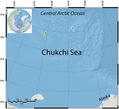
Figure 2. Pictures of (a) the terrestrial 3D laser scanner experiment during the sea ice campaigns and (b) a snow pit with a width and length of ~10 cm and a depth of 15 cm for the hand test of the snow.

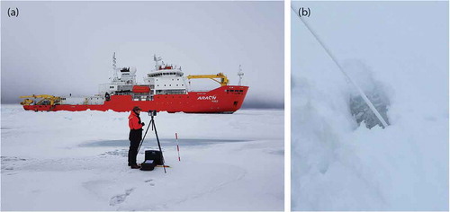
Table 1. Specifications of the terrestrial 3D laser scanner FARO focus3D X130 (FARO Technologies Inc 2014).

Parameter	Value
Range	0.6–130 m
Maximum measurement speed	976,000 points/s
Ranging error	±2 mm at 25 m
Vertical/horizontal field of view	300°/360°
Vertical/horizontal step size	0.009°/0.009°
Observation wavelength	1550 nm

The 3D laser scanner experiments were conducted from 13 August 2017 22:55 Coordinated Universal Time (UTC) to 14 August 2017 01:11 UTC for the 2017 ice campaign, and from 22:08 UTC to 23:48 UTC on 16 August 2018 for the 2018 ice campaign. The 3D measurement points were acquired within an area of approximately 150 m × 100 m in both the campaigns. The height values of the 3D measurements were determined by the altitudes of point clouds, which were measured by the embedded barometric height sensor of the laser scanner. We carried out several scans at different locations, with the distance between successive locations being less than 50 m, and mosaicked them to cover the whole investigated area. This is because the maximum scan range of the used laser scanner is 130 m, but the reflectance of the shortwave infrared radiation of snow and ice is low, and the signals reflected from far away could not be measured. In addition, this procedure can minimize the occluded areas behind ice ridges, where the slope is steeper than the laser depression angle. Each scan was conducted for approximately 20 min, and it took about 1.5 h to cover the whole investigated area in each ice campaign. The mosaic of the scans was produced by matching the 3D points of the reference objects (white spheres with a high reflectance) measured in different scans that overlapped with each other. In this mosaic process, the changes in the absolute locations and heights of the scanner between experiments due to sea ice drift and tidal variations can be neglected.

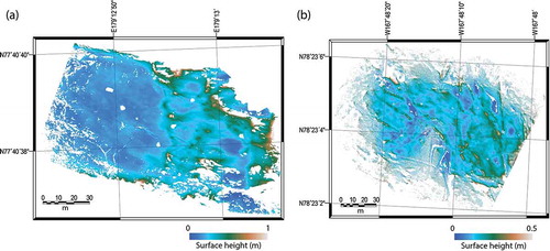
The distributions of the surface heights of sea ice measured by the terrestrial 3D laser scanner in 2017 and 2018 are shown in Figure 3, where they are presented as probability density functions. The surface height represents the height above the ice level. Most surface height values varied between 0 and 0.8 m for 2017, with a mode of 0.16 m (Figure 3(a)). Meanwhile, the surface height values for 2018 were mainly distributed between 0 and 0.4 m, with a mode of 0.15 m (Figure 3(b)). A DSM of the snow-covered sea ice was generated with a grid spacing of 4 cm from the 3D measurement points for each ice campaign (Figure 4). The DSMs derived from the 3D measurements revealed several gaps with no data. The gaps are attributed to the sparse 3D measurement points on occluded areas and melt ponds, which display very low reflectivity of shortwave infrared radiation.

Figure 3. Distributions of surface heights above the ice level for the investigated sea ice, measured by a terrestrial 3D laser scanner as part of (a) 2017 and (b) 2018 sea ice campaigns.

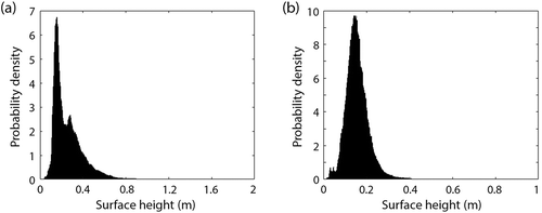
Figure 4. DSMs of the investigated sea ice, generated from the (a) 2017 and (b) 2018 sea ice campaigns. The surface heights of the DSMs show the elevations above the sea ice level.

2.2. TSX and TDX dual-polarimetric SAR data

TSX and TDX, operated by the German Aerospace Center, are equipped with X-band SAR with a center frequency of 9.65 GHz. The TDX is a twin of the TSX and used to measure the accurate elevation of the earth by supplementing the TSX observations. TSX and TDX provide high-resolution images in six different imaging modes with different spatial resolutions: 0.25 m in staring spotlight, 1 m in high-resolution spotlight, 2 m in spotlight, 3 m in the stripmap, 18 m in ScanSAR, and 40 m in ScanSAR wide mode (Werninghaus and Buckreuss 2010). The different imaging modes exhibit different spatial coverages, and the coverage is larger for a lower resolution mode. The nominal revisit cycle of the satellites is 11 days. Among the six imaging modes, high-resolution spotlight, spotlight, and stripmap mode can provide dual-polarimetric data, whereas the others provide single-polarization data only. In this study, TSX and TDX dual-polarimetric (HH and VV) SAR images were acquired in the stripmap mode for the 2017 and 2018 sea ice campaigns on 16 August 2017 and 22 August 2018, respectively (Figure 5). Table 2 shows the details of the TSX and TDX SAR data used in this study. The TSX and TDX SAR data were acquired at different incidence angles: a high incidence angle of 49.5° at the location of the center of the 2017 campaign, and a mid-incidence angle of 36.1° at the location of the center of 2018 campaign.

Figure 5. (a) TerraSAR-X HH-polarized backscattering coefficient image acquired on 16 August 2017. (b) TanDEM-X HH-polarized backscattering coefficient image obtained on 22 August 2018. The red dots represent the locations of the two sea ice campaigns.

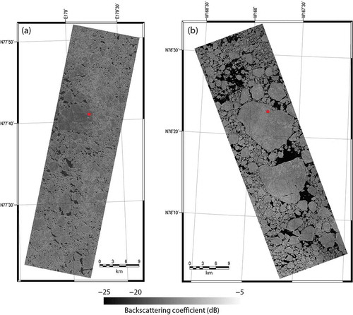
Table 2. Specifications of the TSX and TDX dual-polarimetric SAR data used in this study.

Parameter	2017 sea ice campaign		2018 sea ice campaign
Satellite	TSX		TDX
Center frequency (GHz)	9.65 GHz (X-band)
Date	16 August 2017		22 August 2018
Time (UTC)	18:49		03:47
Acquisition mode	Stripmap
Polarization	HH/VV
Incidence angle (at the center of the study area)		49.5º	36.1º
Noise equivalent sigma zero (NESZ)	−19.86 dB		−23.63 dB

The TSX and TDX dual-polarimetric SAR data were delivered in single look slant range complex (SSC) format. We applied a 5 × 5 Lee filter to the SSC data in order to reduce speckle noise. Then, the backscattering coefficients and polarimetric features were computed from the filtered data. Pixels with a backscattering coefficient below the noise equivalent sigma zero (NESZ) were discarded from the analysis. A detailed description of the computation of the polarimetric features is given in Section 3.

2.3. Helicopter-borne and unmanned aerial vehicle (UAV) photographs

The TSX and TDX SAR data were acquired 1–2 days after the 3D laser scanning experiments. As sea ice continuously drifted, the locations of ice floes during the laser scanning experiments and during SAR data acquisition were different owing to the time differences. The SAR features and DSMs should be co-registered to investigate the surface roughness of sea ice, which is reflected in the polarimetric SAR. However, co-registration between the two datasets is difficult because the fine surface features observed in the DSMs (or in true-color images with the same geometry as the DSMs derived from the scanner) are invisible in the SAR images, which is attributed to the much lower spatial resolution (3 m).

We obtained helicopter (BELL 206 L-3)-borne and UAV (DJI Phantom 4) true-color images with spatial resolutions of 30 and 4 cm, respectively (Hyun et al. 2019; Kim et al. 2019), for the sea ice of each campaign (Figure 6). These airborne images were ortho-mosaicked and used for the co-registration between the DSMs and the SAR data. Tables 3 and 4 show the specifications of the helicopter-borne and UAV imaging setups, respectively (Hyun et al. 2019; Kim et al. 2019). Small sea ice surface features, such as small ridges, are observed in the 3D laser scanning measurements, whereas ponds that are several tens of centimeters in length and width appear in the UAV images; larger features can be seen in both the UAV and helicopter-borne images. Furthermore, large surface features that are several tens of meters in length and width, such as large melt ponds, channels of the melt ponds, cracks, and the IBRV Araon, can be observed in both the helicopter-borne and SAR amplitude images. This shows that co-registration between SAR and helicopter-borne images, helicopter-borne and UAV images, and UAV images and DSMs is possible. This consecutive image co-registration process enables geometric registration between DSMs and SAR data.

Figure 6. (a and d) Mosaics derived from UAV images, (b and e) mosaics derived from helicopter-borne images, and (c and f) TSX and TDX HH-polarized backscattering coefficient images corresponding to the areas of the helicopter-borne mosaics. The upper and lower images were acquired for the 2017 and 2018 sea ice campaigns, respectively. The red and blue polygons in (b), (c), (e), and (f) correspond to the areas of 3D laser scanning experiments and UAV imaging, respectively.

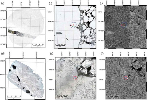
Table 3. Specifications of the helicopter-borne imaging setup.

Helicopter-borne imaging setup	2017 sea ice campaign	2018 sea ice campaign
Start time of image acquisition (UTC)	13 August 2017 23:48:37	21 August 2018 22:28:59
End time of image acquisition (UTC)	14 August 2017 01:03:00	21 August 2018 23:06:16
Altitude of imaging location	Up to 2407 m	Up to 622 m
Digital camera	Canon EOS M6
Image acquisition interval	1 s
Focal length	22 mm
Aperture	F11
Shutter speed	Varies between 1/1000 and 1/3200	Varies between 1/250 and 1/2000
ISO	400

Table 4. Specifications of the UAV imaging setup.

UAV imaging setup	2017 sea ice campaign	2018 sea ice campaign
Start time of image acquisition (UTC)	13 August 2017 22:13:38	22 August 2018 00:55:56
End time of image acquisition (UTC)	13 August 2017 22:17:11	22 August 2018 01:00:02
Altitude of imaging location	Up to 53 m	Up to 45 m
Digital camera	DJI FC330	DJI FC6310
Image acquisition interval	9 s	2 s
Focal length	3.6 mm	8.8 mm
Aperture	F2.8	F7.1
Shutter speed	1/3333 s	1/1250 s
ISO	100

2.4. Sea ice conditions

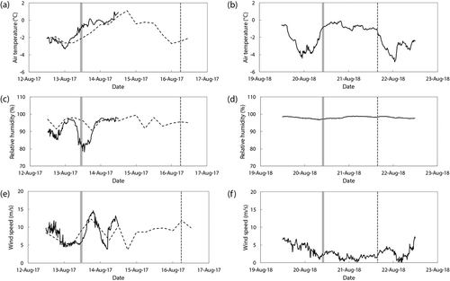
Figure 7 shows the temporal changes in the air temperature, wind speed, and relative humidity for the two ice campaigns that were measured by a meteorological sensor mounted at the foremast of IBRV Araon and predicted by ERA-Interim reanalysis data (Dee et al. 2011). After ice campaign on 14 August 2017, the IBRV Araon left the investigated ice floe, and the weather conditions in the area of study could not be measured by using the meteorological sensor. Therefore, we used the 6-hr fields of the ERA-Interim reanalysis data with a grid size of 0.125° × 0.125°. The meteorological parameters predicted by the ERA-Interim reanalysis data for the 2017 ice campaign are depicted as dotted lines in Figure 7. The ERA-Interim reanalysis data have been widely used to study weather conditions and their changes in the Arctic (Bengtsson et al. 2011; Maksimovich and Vihma 2012; Kapsch et al. 2014; Mortin et al. 2016; Han and Kim 2018). Even though the ERA-Interim reanalysis data have coarse spatial and temporal resolutions, the predicted summer wind speed (Lindsay et al. 2014; Wesslén et al. 2014), relative humidity (Wesslén et al. 2014), and air temperature when it is higher than −25°C (Wang et al. 2019) in the Arctic Ocean were reported to be in good agreement with in situ observations. For the 2017 ice campaign, the reanalysis fields showed small root mean square deviations of 0.76°C, 5.95%, and 2.17 m/s for air temperature, relative humidity, and wind speed, respectively, when compared with measurements of the meteorological sensor before 15 August 2017. Therefore, the ERA-Interim reanalysis fields can be adequately used for weather analysis during the period without in situ meteorological measurements. The relative humidity on 13 August 2017 from the reanalysis fields was 10–15% higher than that measured by the meteorological sensor mounted at the IBRV Araon. This was possibly due to the low temporal resolution of the ERA-Interim data. The relative humidity was higher than 80% during the ice campaigns. Nevertheless, the air was dry because the saturated water vapor was low at the low temperatures.

The drilling-derived sea ice thickness was 1.00 and 1.01 m in the 2017 and 2018 ice campaigns, respectively, which suggest that it was most likely first-year sea ice. The ice floes in the study area in both ice campaigns were covered with 10–37 cm depth of snow, which was measured using a ruler at the locations of the laser scanning experiments. We could not quantitatively determine the wetness of the snow cover on sea ice because the snow properties were not measured, except for the depth. The snow condition in both ice campaigns was estimated by hand test. The hand test was conducted both at the surface and in a snow pit (Figure 2(b)). The snow was loose from the surface to the bottom of the pit and did not stick together well, suggesting that the entire snow cover on the sea ice was dry. Snow on the sea ice can melt rapidly in summer and become wet. However, if the air temperature drops sharply, the snow can refreeze and have a very low level of wetness. During the sea ice campaigns, the air temperature tended to decrease the day prior to the field survey (Figure 7(a-b)). In particular, during the 2018 sea ice campaign, the air temperature was observed to drop sharply from 0°C to −4°C for 12 hours the day prior to the field survey (Figure 7(b)). This suggests the possibility that the snow cover on the sea ice refroze prior to the survey and, therefore, became dry.

Figure 7. Temporal variations in the (a and b) air temperature, (c and d) wind speed, and (e and f) humidity for the 2017 and 2018 sea ice campaigns. In (a), (c), and (e), the solid and dotted lines indicate the measurements of the meteorological sensor mounted on IBRV Araon and the predictions based on the ERA-Interim reanalysis fields, respectively. The gray-colored shadowing boxes and the vertical dotted lines indicate the times of terrestrial 3D laser scanning experiments and SAR data acquisitions, respectively.

3. Methodology

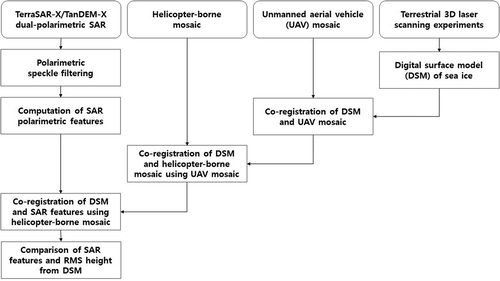
This section presents the methodology for computing the SAR features from the TSX and TDX dual-polarimetric data and a comparison of these features with the RMS height of the snow-covered first-year sea ice measured by the terrestrial 3D laser scanner. Figure 8 shows a flowchart of data processing.

Figure 8. Process flow of the investigation of the surface roughness signatures of sea ice in TSX/TDX X-band dual-polarimetric SAR features.

3.1. Computation of SAR features from TSX and TDX dual-polarimetric data

For this study, we used a 2 × 2 coherency matrix ($T_2$) for the TSX and TDX dual-polarimetric SAR data (Lee and Pottier 2009):

(1) $T_2=\frac{1}{\sqrt{2}}\left[\begin{array}{cc}{<\left|S_{HH}+S_{VV}\right|}^2>& <\left(S_{HH}+S_{VV}\right){\left(S_{HH}-S_{VV}\right)}^{\ast }>\\ <\left(S_{HH}-S_{VV}\right){\left(S_{HH}+S_{VV}\right)}^{\ast }>& <{\left|S_{HH}-S_{VV}\right|}^2>\end{array}\right]$(1)

where $S_{PP}$ is the element of the complex scattering matrix and the superscript * indicates complex conjugation. The subscript PP indicates transmitted and received polarizations and < > represents the ensemble average of the complex product. The backscattering coefficients for HH (${\sigma }_{HH}^0$) and VV (${\sigma }_{VV}^0$) polarizations in the decibel scale (dB) were derived from the filtered SSC data. In addition to ${\sigma }_{HH}^0$ and ${\sigma }_{VV}^0$, three features―co-polarization ratio in dB, co-polarization phase difference, and co-polarization correlation coefficient ―were derived from the TSX and TDX dual-polarimetric SAR data. The co-polarization ratio (${\gamma }_{VVHH}$), co-polarization phase difference ($\phi$), and co-polarization correlation coefficient ($\rho$) were calculated as

(2) ${\gamma }_{VVHH}=\frac{<S_{VV}{S}_{VV}^{\ast }>}{<S_{HH}{S}_{HH}^{\ast }>}$(2)

(3) $\phi ={tan}^{-1}\left[\frac{im<S_{HH}{S}_{VV}^{\ast }>}{re<S_{HH}{S}_{VV}^{\ast }>}\right]$(3)

(4) $\rho =\left|\frac{<S_{HH}{S}_{VV}^{\ast }>}{\sqrt{<S_{HH}{S}_{HH}^{\ast }{S}_{VV}{S}_{VV}^{\ast }>}}\right|$(4)

where | | stands for the modulus of the complex product.

The SAR features for the two ice campaigns derived from the X-band dual-polarimetric data are shown in Figure 9. All the SAR features were projected onto a Universal Transverse Mercator (UTM) projection (Zone 60 North for the 2017 campaign and Zone 3 North for the 2018 campaign) with a spatial resolution of 3 m.

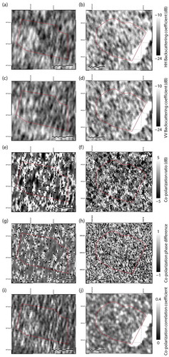
Figure 9. The SAR features investigated in this study. (a and b) Backscattering coefficient in HH polarization, (c and d) backscattering coefficient in VV polarization, (e and f) co-polarization ratio, (g and h) co-polarization phase difference, and (i and j) co-polarization correlation coefficient. The SAR features on the left are for the 2017 ice campaign and those on the right are for the 2018 ice campaign. The red polygons correspond to the areas of 3D laser scanning experiments.

3.2. Co-registration of DSMs and SAR features

The DSMs derived from the 3D laser scanner were projected onto the same geometry as the SAR features using the information of scanner positions that were determined by a ground-positioning system sensor that was integrated into the scanner. Although the DSMs and SAR features were projected onto the same projection, they should be co-registered owing to the continuous drift of sea ice during the time between the two data acquisitions.

As the surface features observed in the DSMs are not easily seen in the SAR intensity images, owing to the difference in spatial resolution, we used the helicopter-borne and UAV images to enable co-registration of the two datasets. In this study, the thin plate spline method (Goshtasby 1988) was used for co-registration of different images in 2-D (x- and y-coordinate). The thin plate spline method, which has been widely used for image transformation, interpolates a surface that passes through a set of control points (CPs) with high accuracy and speed. The thin plate spline method is appropriate for the transformation of remote sensing images with nonlinear and local geometric distortions and can achieve high performance when a small number of CPs are used (Bentoutou et al., 2005; Zagorchev and Goshtasby 2006; Du et al. 2008). First, the helicopter-borne and UAV images were ortho-mosaicked using PhotoScan software (Agisoft LLC, St. Petersburg, Russia) and Pix4D 4.1.24 software (Pix4D SA, Lausanne, Switzerland), respectively, and projected onto the UTM projection (e.g. the same projection with the DSMs and SAR data for each ice campaign). Through visual inspection, we selected several CPs of textured ice surface features (e.g. edges of melt ponds, cracks, and the IBRV Araon) from the helicopter-borne mosaics and the TSX/TDX HH-polarized amplitude images (6 CPs for 2017 and 8 CPs for 2018). The helicopter-borne mosaics were co-registered to the SAR images using the thin plate spline method and the CPs. The RMS values of the residuals of the CPs between the two datasets were calculated as 1.76 and 1.53 m for the 2017 and 2018 ice campaigns, respectively. We then co-registered the UAV mosaics to the helicopter-borne mosaics, which were geometrically matched to the HH-polarized SAR amplitude images by selecting 9 CPs for 2017 and 5 CPs for 2018, in which the RMS values of the residuals of the CPs were calculated as 0.44 and 0.13 m for 2017 and 2018, respectively. Finally, the DSMs were co-registered to the transformed UAV mosaics by selecting 15 CPs for 2017 and 12 CPs for 2018. The RMS values of the residuals of the CPs between the DSMs and the UAV mosaics were calculated as 0.36 and 0.06 m for the 2017 and 2018 ice campaigns, respectively.

Through the consecutive co-registration process, the DSMs were geometrically matched to the geometry of the SAR features. The final errors of co-registration between the DSMs and SAR data were estimated as 1.85 m for 2017 and 1.54 m for 2018 by considering the propagated RMS values of the residuals of CPs that were calculated from the consecutive image co-registration process.

3.3. Correlation analysis of DSM-derived RMS height and SAR features

The values of the RMS height of the snow-covered sea ice were computed from the DSMs using a 375 × 375 pixel non-overlapping stepping window, which corresponds to a rectangular area of 15 m × 15 m. If more than 20% of no-data pixels were included in the 375 × 375 pixel window of the DSMs, the RMS height was not computed for the given window and not used in the analysis. We subsequently compared the RMS height with each of the averaged SAR features that were computed within a 5 × 5 pixel non-overlapping stepping window for the corresponding area. We could have made the grid size of the RMS height finer than 15 m × 15 m based on the very high resolution of the SAR images and DSMs. Nevertheless, in the RMS height investigation, the reasons for setting the grid size to 15 m × 15 m and not to the grid size of the SAR features (3 m × 3 m) were to extract the number of samples necessary for the analysis and to reduce the effect of co-registration error of ~2 m between the DSMs and SAR features in the comparison of the two datasets.

The RMS height measured by the terrestrial 3D laser scanner represents the surface roughness of the snow cover on sea ice and not that of the snow/ice interface. The roughness of the snow cover may be different from that of the snow/ice interface, especially for very smooth or very rough ice (Manninen 1997; Johansson et al. 2017). Nevertheless, the RMS height of the snow cover is strongly correlated with that of the ice under it and can be used as an effective measure of the surface roughness of snow-covered sea ice (Andreas et al. 1993). In this study, we assume that the surface roughness of the snow cover on sea ice is equal to that of the snow/ice interface, i.e. sea ice surface roughness. The snow cover on sea ice in both ice campaigns was estimated as dry based on hand test. For dry snow-covered sea ice, microwave backscattering from a snow surface can be negligible because of a very small difference in permittivity between air and snow (Kim, Onstott, and Moore 1984; Nghiem et al. 1995). The volume scattering from the snowpack is very small under dry snow condition. Meanwhile, the permittivity contrast of the snow/ice interface is much higher than that of the air/snow interface and snowpack, and dominant microwave backscattering occurs on the snow/ice interface (Kim, Onstott, and Moore 1984; Nghiem et al. 1995). Dierking (2013) and Paul et al. (2015) showed that the X-band microwave is transparent to dry snowpack due to low dielectric permittivity. The penetration depth of microwave at X-band is about 1 m for dry snow (Dierking, Lang, and Busche 2017; Ulaby, Moore, and Fung 1982). The snow depth of both ice campaigns was measured at 10–37 cm, which could be transparent in the TerraSAR-X and TanDEM-X observations. Therefore, the X-band SAR signals can reflect the surface structure of sea ice and can be compared to the RMS height measured by the laser scanner.

The characteristics of the X-band dual-polarimetric SAR features on the surface roughness of the snow-covered sea ice were investigated by analyzing the 1:1 correlation between the RMS height values of the sea ice surface and the SAR features. In this study, Spearman’s rank correlation coefficient (R) was computed to establish the relationship between RMS height and SAR features. Spearman’s rank correlation coefficient is a non-parametric statistic for measuring the degree of association between two variables that are not normally distributed and is appropriate for the correlation analysis of variables that are measured on a scale that is at least ordinal. This coefficient is based on the assumption that two variables exhibit a monotonic relationship. By selecting this coefficient, assumptions of a linear relationship between RMS height and SAR features can be avoided, and the non-linear aspect of the relationship can be explored.

4. Results and discussion

4.1. Correlations between intensity-based features and RMS height

The RMS heights derived from the terrestrial 3D laser scanner ranged from 1.5 to 17.9 cm for the 2017 campaign and from 2.2 to 6.9 cm for the 2018 campaign, as shown in the scatterplots of the RMS height and SAR features (Figure 10–13). In microwave remote sensing, surface roughness can be scaled based on RMS height and microwave wavelength. If the RMS height is much lower than the observation wavelength, a surface is defined as having microscale roughness, which is a governing factor of the radar backscattering from the surface (Fors et al. 2016b). Surface roughness with an RMS height similar to or larger than the observation wavelength is defined as macroscale roughness, which also exhibits a great influence on radar backscattering (Fors et al. 2016b). Most of the values of the RMS height of the snow-covered sea ice investigated in both the campaigns were larger than the wavelength of the TSX and TDX X-band SAR (3.1 cm), and we could confirm that the sea ice surface roughness is depicted as macroscale roughness.

If there are hoar or brine layers with high permittivity in the snow cover, the penetration depth of microwave decreases (Kim, Onstott, and Moore 1984; Nghiem et al. 1995; Fuller et al. 2014) and the backscattering in HH polarization is significantly greater than that in VV polarization (Geldsetzer and Yackel 2009). We could not measure the physical properties of the snow cover, except its depth, and thus the influence of the snowpack on the X-band backscattering was estimated by analyzing the scatterplots of backscattering coefficient in HH and VV polarizations (${\sigma }_{HH}^0$ and ${\sigma }_{VV}^0$) for both ice campaigns (Figure 10). The values of ${\sigma }_{HH}^0$ and ${\sigma }_{VV}^0$ are similar for both ice campaigns. Based on this, we estimated that the scattering from the snow surface and in the snowpack is smaller than that on the snow/ice interface because of dry snow conditions, and the measured backscattering can reflect the roughness of the sea ice surface under the snow cover.

We analyzed the correlation between the RMS height of the snow-covered sea ice and the corresponding SAR features. Figure 10(a-b) show the scatterplots of the RMS height and the co-polarization backscattering coefficients for the 2017 ice campaign. In the scatterplots, a p-value below 0.05 means that the correlation is statistically significant at a confidence level of 95%. ${\sigma }_{HH}^0$ and ${\sigma }_{VV}^0$ show low correlations with the RMS height, with R values of −0.583 and −0.585, respectively. However, a decreasing trend is observed for the RMS height up to 5 cm. Radar backscattering typically increases with increasing surface roughness of sea ice owing to double- or multi-bounce scattering (Mäkynen and Hallikainen 2004; Gill and Yackel 2012; Moen et al. 2013; Zhang et al. 2016). This positive relationship is mainly attributed to the microscale surface roughness (Fors et al. 2016b; Zhang et al. 2016). On the other hand, for a surface with macroscale roughness, the intensity of radar backscattering can decrease with increasing RMS height, because the angular curve of scattering is expected to be more isotropic and the magnitude of the backscattered power is smaller than that of a surface with microscale roughness (Fung and Chen 2010). Therefore, the negative relationship between the co-polarized backscattering coefficients and the RMS height could be attributed to the macroscale surface roughness of the snow-covered sea ice.

For an RMS height larger than 5 cm, ${\sigma }_{HH}^0$ and ${\sigma }_{VV}^0$ hardly change with an increasing RMS height. This is possibly attributed to the high incidence angle of the TSX SAR data (49.5°). The radar backscattering power decreases as the incidence angle increases when the physical and structural properties of a target do not change, and higher incidence angles lead to higher NESZ values. The scatterplots in (Figure 10(a-b)) show that ${\sigma }_{HH}^0$ and ${\sigma }_{VV}^0$ decrease and then approach the NESZ value of the TSX SAR data (−19.86 dB) around the RMS height of 5 cm. This implies that the large roughness of the snow-covered sea ice cannot be characterized based on the magnitude of backscattering of X-band SAR data at high incidence angles.

In the location of the 2017 campaign, the air temperature was above 0°C 1 day before the TSX SAR data acquisition, and the wind speed was about 10 m/s. These might have changed the wetness and morphology of the snow cover of the sea ice between the time of the terrestrial 3D laser scanning experiments and the time of SAR acquisition, which could be a cause of the low correlation observed between the co-polarized backscattering coefficients and the RMS height. However, since the air temperature of 0–1°C lasted for only a short period of time, it would have had little impact on the wetness and dielectric property of the snow cover. It is assumed that the winds also exhibited a small effect on the changes in the surface roughness of the snow-covered sea ice. This is because strong relationships with the co-polarized backscattering coefficients were observed for RMS heights lower than 5 cm, where the backscattering coefficients were at least 1 dB higher than the NESZ.

Figure 10. Scatterplots of backscattering coefficients in HH (${\sigma }_{HH}^0$) and VV polarizations (${\sigma }_{VV}^0$) versus RMS height for the (a and b) 2017 and (c and d) 2018 sea ice campaigns. The values enclosed within parentheses in figures (a) and (b) represent the R and p values for RMS heights lower than 6.9 cm. The horizontal dotted line indicates the level of NESZ of SAR data.

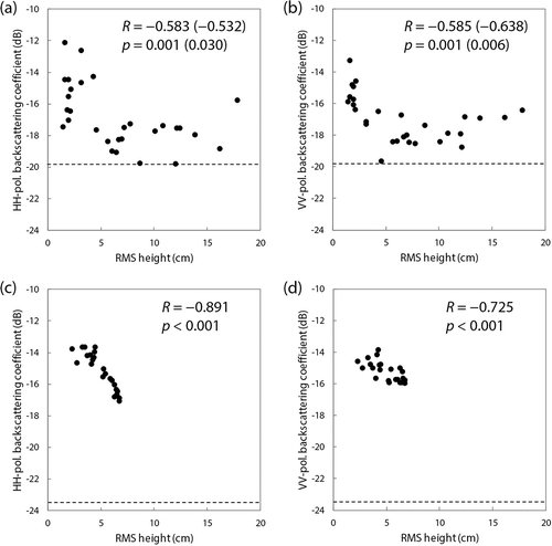
The TDX SAR data for the 2018 ice campaign were acquired at a mid-incidence angle (36.1°). The ${\sigma }_{HH}^0$ and RMS height for 2018 showed a very strong negative correlation, with an R value of −0.891, which was due to the macroscale surface roughness (Figure 10(c)). ${\sigma }_{VV}^0$ was also strongly correlated with the RMS height of sea ice (R value of −0.725 (Figure 10(d))). The correlations between the co-polarized backscattering coefficients and the RMS height for the 2018 ice campaign were much stronger than those for the 2017 ice campaign, which would be attributed to the difference in the distributions of the RMS height values. The maximum RMS height value for 2018 was only 6.9 cm, but the maximum RMS height for 2017 was up to 17.9 cm. The values of ${\sigma }_{HH}^0$ and ${\sigma }_{VV}^0$ for 2017 were close to the NESZ at RMS heights higher than 5 cm, which contributed to the low correlation observed between the backscattering coefficients and the RMS height. For an RMS height lower than 6.9 cm (which is the observed maximum for 2018) for 2017, however, the co-polarized backscattering coefficients and the RMS height showed weak correlations (Figure 10(a-b)). The air temperature was below 0°C, and a gentle wind was observed during the terrestrial 3D laser scanning experiments and TDX SAR data acquisition, which would not change the surface roughness characteristics of the snow-covered sea ice and would contribute to the strong correlations observed between the co-polarized backscattering coefficients and the RMS height.

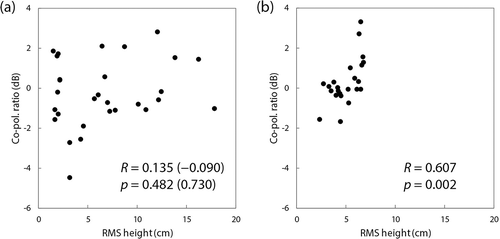
(Figure 11(a-b)) show the scatterplots of the RMS height of the snow-covered sea ice and ${\gamma }_{VVHH}$ for the ice campaigns conducted in 2017 and 2018, respectively. ${\gamma }_{VVHH}$ depends on the surface roughness, dielectric constant of the surface, and dominant scattering mechanism of sea ice (Mäkynen and Hallikainen 2004; Scharien et al. 2012). For the 2017 ice campaign, the correlation between ${\gamma }_{VVHH}$ and RMS height was very weak (R values of 0.135 for all RMS height values and −0.090 for RMS heights <6.9 cm), which was attributed to the influence of a low backscattering close to the NESZ. The ${\gamma }_{VVHH}$ and RMS height of sea ice for the 2018 ice campaign showed a higher but not stronger correlation (R value of 0.607), although the backscattering coefficients were higher than the NESZ value because of the mid-incidence angle. Previous studies with C-band showed that ${\gamma }_{VVHH}$ increases with increasing surface roughness of sea ice (Drinkwater et al. 1991; Mäkynen and Hallikainen 2004), whereas Wakabayashi et al. (2004) used L-band polarimetric SAR data and reported that the surface roughness contribution to co-polarized backscatter is canceled in the calculation of ${\gamma }_{VVHH}$. (Figure 11(b)) shows that the ${\gamma }_{VVHH}$ at the X-band with a mid-incidence angle does not reflect the macroscale surface roughness of the snow-covered sea ice.

Figure 11. Scatterplots of co-polarization ratio (${\gamma }_{VVHH}$) versus RMS height for the (a) 2017 and (b) 2018 sea ice campaigns. The values enclosed within parentheses in figure (a) represent the R and p values for RMS heights lower than 6.9 cm.

4.2. Correlations between polarimetric features and RMS height

The relationships of RMS height to $\phi$ and $\rho$ for the 2017 and 2018 ice campaigns are shown in (Figures 12and 13) respectively. $\phi$ and $\rho$ were reported to be sensitive to the surface roughness of sea ice and to decrease with increasing roughness (Wakabayashi et al. 2004; Gill and Yackel 2012; Moen et al. 2013; Fors et al. 2016b). For the 2017 ice campaign, however, $\phi$ and $\rho$ showed R values less than 0.6 with the RMS height of sea ice (Figures 12aand 13a). This is because the changes in $\phi$ and $\rho$ caused by surface roughness are small at a high incidence angle (Wakabayashi et al. 2004). The scattering components close to the noise level due to the high incidence angle can also contribute to the low correlations.

Figure 12. Scatterplots of co-polarization phase difference ($\phi$) versus RMS height for the (a) 2017 and (b) 2018 sea ice campaigns. The values enclosed within parentheses in figure (a) represent the R and p values for RMS heights lower than 6.9 cm.

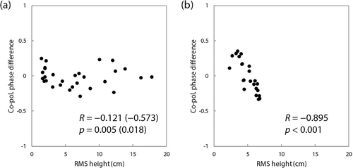
Figure 13. Scatterplots of co-polarization correlation coefficient ($\rho$) versus RMS height for the (a) 2017 and (b) 2018 sea ice campaigns. The values enclosed within parentheses in figure (a) represent the R and p values for RMS heights lower than 6.9 cm.

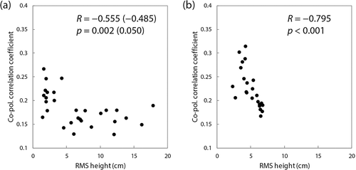
$\phi$ and $\rho$ were reported to show good correlations with the sea ice surface roughness at a lower incidence angle (Wakabayashi et al. 2004). For the ice campaign conducted in 2018, the $\phi$ and $\rho$ derived from the mid-incidence angle TDX SAR data were strongly correlated with the RMS height of sea ice, showing R values of −0.895 and −0.795, respectively (Figures 12b and 13b). These strong relationships are in agreement with the results that have been reported in previous studies (Wakabayashi et al. 2004; Gill and Yackel 2012; Brekke, Grahn, and Doulgeris 2015; Fors et al. 2016b).

4.3. Feasibility of using X-band dual-polarimetric SAR for sea ice surface roughness investigations

The intensity- and polarimetry-based features derived from the TSX and TDX dual-polarimetric SAR data were compared with the RMS height of the first-year sea ice with dry snow cover measured by the terrestrial 3D laser scanning experiments in the MIZ of the Chukchi Sea in summer. The X-band dual-polarimetric SAR features derived at a high incidence angle were not significantly correlated with the RMS height (<17.9 cm), which was mainly because of low radar backscattered signals that were observed close to the noise level. Meanwhile, the SAR features derived at a mid-incidence angle, except for the co-polarization ratio, showed a statistically significant correlation with the RMS height (<6.9 cm) of the investigated sea ice surface. At the mid-incidence angle, backscattering at HH polarization and co-polarization phase difference was the most promising among the intensity- and polarimetry-based SAR features, respectively, for investigation of the RMS height of the snow-covered sea ice with macroscale surface roughness in summer.

The dual-polarimetric X-band SAR features obtained at the mid-incidence angle (for the 2018 ice campaign) were found to be more feasible for characterizing the summer sea ice with dry snow cover for RMS heights lower than 7 cm than those derived at the high incidence angle (for the 2017 ice campaign). However, values of RMS height higher than 7 cm were not observed in the 2018 campaign, and we could not investigate the relationship between the SAR features obtained at the mid-incidence angle and a higher RMS height. For the late-summer first-year sea ice, the C-band co-polarized backscattering coefficients and co-polarization ratio at a mid-incidence angle (38.2°) were strongly negatively correlated with the RMS height for height values lower than 30 cm (Fors et al. 2016b). In our observations, the X-band backscattering coefficients at the mid-incidence angle clearly showed an inverse relationship with the RMS height and were at least 6 dB higher than the noise level (Figure 9(c-d)). For RMS height values lower than 7 cm, the SAR features, except co-polarization ratio, showed more significant correlations with the RMS height at the mid-incidence angle than at the high incidence angle. Therefore, the X-band radar backscattering at a mid-incidence angle may be significantly correlated with the RMS height as the latter increases to at least the observed maximum for 2017 (17.9 cm). Further sea ice campaigns and acquisitions of mid-incidence angle SAR data, or radar backscattering modeling studies, are required for more accurate analysis of the relationships, but these are left for future work.

Surface roughness can vary greatly in space, even within a single ice floe. However, the area of sea ice over which the RMS height was analyzed was small (100 m × 150 m for each ice campaign), and might not have been enough to investigate the general characteristics of the SAR features for the macroscale surface roughness of sea ice. Nevertheless, the measured RMS height, ranging from 2 to 17 cm, seemed to reflect the macroscale surface roughness corresponding to the X-band wavelength. The errors in co-registration between the sea ice DSMs, UAV images, helicopter-borne images, and SAR images (<2 m) can be an impediment to accurate analysis of the relationship between the SAR features and the RMS height of sea ice. However, they were very small compared to the grid size in the RMS height investigation (15 m); thus, the results of statistical analysis of the correlation between the SAR features and the RMS height can be considered reasonable.

The results of the correlation analysis showed that the X-band SAR features at the mid-incidence angle are superior to those at the high incidence angle for investigating the RMS height of snow-covered first-year sea ice. In addition, we were able to identify which X-band features are sensitive to the macroscale surface roughness of sea ice. However, this study has limitations in the investigation of sea ice surface roughness. First, only one SAR data was acquired from each of the two sea ice campaigns. The ice campaigns were conducted in different locations and at different times, so the surface roughness of sea ice and the weather conditions were also different. For more accurate analysis of the correlation between sea ice surface roughness and SAR features by incidence angles, at least two SAR data with different incidence angles should be acquired from the same ice campaign. To this end, we tried to acquire two or more SAR images with different incidence angles and polarizations by predicting the drift of sea ice. However, the drift of sea ice was different from what was predicted, and the SAR imaging of the sea ice campaigns failed. The other limitation is the lack of information on snow properties such as density, wetness, and grain size, which significantly influences the microwave scattering mechanism and the interpretation of the relationship between SAR features and sea ice roughness. Unfortunately, only the depth of snow was measured during the sea ice campaigns, and it was estimated that the snow was dry by hand test. Our future works will include investigation of signals of Arctic summer sea ice surface roughness in SAR features at various frequencies and incidence angles in combination with information on the physical properties of snow and ice in future sea ice campaigns.

5. Conclusion

The characteristics of the macroscale surface roughness signatures of the sea ice with dry snow cover on the Chukchi Sea in summer were analyzed in terms of the RMS height in dual-polarimetric X-band SAR by using a 3D terrestrial laser scanner, a UAV, and a helicopter, and two TSX/TDX dual-polarimetric SAR datasets with different radar incidence angles. The 3D laser scanning experiments were conducted on the snow-covered sea ice to acquire very-high-resolution DSMs of them, which were used to compute the RMS heights of sea ice based on a grid size of 15 m. The co-polarized backscattering coefficients, co-polarization ratio, and co-polarization correlation coefficient of the snow-covered sea ice were computed from the TSX/TDX X-band dual-polarimetric SAR data, which were geometrically matched to the DSMs through a consecutive co-registration process by using the UAV and helicopter-borne photographs. The errors of the co-registration between the DSMs and SAR data were smaller than 2 m, which enabled a comparison of the SAR features and the RMS height of sea ice at a scale of 15 m × 15 m.

The SAR features derived from the X-band dual-polarimetric SAR data at a high incidence angle (49.5°) were not statistically correlated with the RMS height of the snow-covered sea ice. This may have been possibly caused by the low radar backscattering close to the noise level, which is due to the high incidence angle. Meanwhile, the SAR features of the X-band dual-polarimetric data acquired at a mid-incidence angle (36.1°), except for the co-polarization ratio, showed a statistically strong correlation with the RMS height of the snow-covered sea ice. The backscattering coefficient in HH polarization and the co-polarization phase difference was the most promising among the intensity- and polarimetry-based SAR features, respectively, and described the RMS height of the snow-covered sea ice with macroscale surface roughness. Our results demonstrate that X-band dual-polarimetric SAR features at a mid-incidence angle can reflect the surface roughness characteristics of snow-covered first-year sea ice in summer and can potentially be used for estimation of the roughness of sea ice in terms of RMS height.

Sea ice surface roughness can vary spatially and temporally even for the same ice floe. To investigate the spatiotemporal characteristics of sea ice surface roughness, satellite polarimetric SAR and field observation data need to be obtained for various regions and seasons. More satellite polarimetric SAR and in situ observation data will not only enhance our understanding of the sea ice roughness signatures in SAR but also enable the development of sea ice roughness estimation models based on SAR observations.

Acknowledgements

This research was supported by the Korea Polar Research Institute (KOPRI) through grant PE20080.

Disclosure statement

We declare that there are no conflicts of interest in the research.

Additional information

Funding

This work was supported by the Korea Polar Research Institute [PE20080].

References

- Andreas, E. L., M. A. Lange, S. F. Ackley, and P. Wadhams. 1993. “Roughness of Weddell Sea Ice and Estimates of the Air-ice Drag Coefficient.” Journal of Geophysical Research 98 (C7): 12439–12452. doi:10.1029/93JC00654.
- Bengtsson, L., K. I. Hodges, S. Koumoutsaris, M. Zahn, and N. Keenlyside. 2011. “The Changing Atmospheric Water Cycle in Polar Regions in a Warmer Climate.” Tellus A: Dynamic Meteorology and Oceanography 63 (5): 907–920. doi:10.1111/j.1600-0870.2011.00534.x.
- Bentoutou, Y., N. Taleb, K. Kpalma, and J. Ronsin. 2005. “An Automatic Image Registration for Applications in Remote Sensing.” IEEE Transactions on Geoscience and Remote Sensing 43 (9): 2127–2137. doi:10.1109/TGRS.2005.853187.
- Bi, H., X. Yang, Z. Li, and X. Zhou. 2013. “Sea Ice Small-scale Surface Roughness Estimation Based on AMSR-E Observations.” International Journal of Remote Sensing 34 (12): 4425–4448. doi:10.1080/01431161.2013.779043.
- Brekke, C., J. Grahn, and A. P. Doulgeris. 2015. “Quad-polarimetric SAR for Roughness and Deformation Characterization of Sea Ice at Hopen.” Paper Presented at the POLinSAR2015, Frascati, Italy, 26–30 January 2015.
- Castellani, G., M. Losch, M. Ungermann, and R. Gerdes. 2018. “Sea-ice Drag as a Function of Deformation and Ice Cover: Effects on Simulated Sea Ice and Ocean Circulation in the Arctic.” Ocean Modelling 128: 48–66. doi:10.1016/j.ocemod.2018.06.002.
- Castellani, G., C. Lüpkes, S. Hendricks, and R. Gerdes. 2014. “Variability of Arctic Sea-ice Topography and Its Impact on the Atmospheric Surface Drag.” Journal of Geophysical Research: Oceans 119: 6743–6762. doi:10.1002/2013JC009712.
- Dabboor, M., and T. Geldsetzer. 2014. “Towards Sea Ice Classification Using Simulated RADARSAT Constellation Mission Compact Polarimetric SAR Imagery.” Remote Sensing of Environment 140: 189–195. doi:10.1016/j.rse.2013.08.035.
- Dee, D. P., S. M. Uppala, A. J. Simmons, P. Berrisford, P. Poli, S. Kobayashi, U. Andrae, et al. 2011. “The ERA-Interim Reanalysis: Configuration and Performance of the Data Assimilation System.” Quarterly Journal of the Royal Meteorological Society 137 (656): 553–597. doi:10.1002/qj.828.
- Deems, J. S., T. H. Painter, and D. C. Finnegan. 2013. “Lidar Measurement of Snow Depth: A Review.” Journal of Glaciology 59 (215): 467–479. doi:10.3189/2013JoG12J154.
- Dierking, W. 2013. “Sea Ice Monitoring by Synthetic Aperture Radar.” Oceanography 26 (2): 100–111. doi:10.5670/oceanog.2013.33.
- Dierking, W., and T. Busche. 2006. “Sea Ice Monitoring by L-band SAR: An Assessment Based on Literature and Comparisons of JERS-1 and ERS-1 Imagery.” IEEE Transactions on Geoscience and Remote Sensing 44 (2): 957–970. doi:10.1109/TGRS.2005.861745.
- Dierking, W., O. Lang, and T. Busche. 2017. “Sea Ice Local Surface Topography from Single-pass Satellite InSAR Measurements: A Feasibility Study.” The Cryosphere 11 (4): 1967–1985. doi:10.5194/tc-11-1967-2017.
- Drinkwater, M., R. Kwok, D. P. Winebrenner, and E. Rignot. 1991. “Multifrequency Polarimetric Synthetic Aperture Radar Observations of Sea Ice.” Journal of Geophysical Research 96 (C11): 20679–20698. doi:10.1029/91JC01915.
- Du, Q., N. Raksuntorn, A. Orduyilmaz, and L. M. Bruce. 2008. “Automatic Registration and Mosaicking for Airborne Multispectral Image Sequences.” Photogrammetric Engineering and Remote Sensing 74 (2): 169–181. doi:10.14358/PERS.74.2.169.
- Eicken, H., T. C. Grenfell, D. K. Perovich, J. A. Richter-Menge, and K. Frey. 2004. “Hydraulic Controls of Summer Arctic Pack Ice Albedo.” Journal of Geophysical Research 109 (C8): C08007. doi:10.1029/2003JC001989.
- Eriksson, L. E. B., K. Borenäs, W. Dierking, A. Berg, M. Santoro, P. Pemberton, H. Lindh, and B. Karlson. 2010. “Evaluation of New Spaceborne SAR Sensors for Sea-ice Monitoring in the Baltic Sea.” Canadian Journal of Remote Sensing 36 (sup1): S56–S73. doi:10.5589/m10-020.
- FARO Technologies Inc. 2014. FARO Laser Scanner Focus3D X130 Manual. Lake Mary, FL: FARO Technologies Inc.
- Fisher, R., and V. I. Lytle. 1998. “Atmospheric Drag Coefficients of Weddell Sea Ice Computed from Roughness Profiles.” Annals of Glaciology 27: 455–460. doi:10.3189/1998AoG27-1-455-460.
- Fors, A. S., C. Brekke, A. P. Doulgeris, T. Eltoft, A. H. H. Renner, and S. Gerland. 2016a. “Late-summer Sea Ice Segmentation with Multi-polarisation SAR Features in C and X Band.” The Cryosphere 10 (1): 401–415. doi:10.5194/tc-10-401-2016.
- Fors, A. S., C. Brekke, S. Gerland, A. P. Doulgeris, and J. F. Beckers. 2016b. “Late Summer Arctic Sea Ice Surface Roughness Signatures in C-band SAR Data.” IEEE Journal of Selected Topics in Applied Earth Observations and Remote Sensing 9 (3): 1199–1215. doi:10.1109/JSTARS.2015.2504384.
- Fuller, M. C., T. Geldsetzer, J. P. S. Gill, J. J. Yackel, and C. Derksen. 2014. “C‐band Backscatter from a Complexly‐layered Snow Cover on First‐year Sea Ice.” Hydrological Processes 28 (16): 4614–4625. doi:10.1002/hyp.10255.
- Fung, A. K., and K. Chen. 2010. Microwave Scattering and Emission Models for Users. Norwood, MA: Artech House.
- Geldsetzer, T., and J. J. Yackel. 2009. “Sea Ice Type and Open Water Discrimination Using Dual Co-polarized C-band SAR.” Canadian Journal of Remote Sensing 35 (1): 73–84. doi:10.5589/m08-075.
- Gill, J. P. S., and J. J. Yackel. 2012. “Evaluation of C-band SAR Polarimetric Parameters for Discrimination of First-year Sea Ice Types.” Canadian Journal of Remote Sensing 38 (3): 306–323. doi:10.5589/m12-025.
- Goshtasby, A. 1988. “Registration of Images with Geometric Distortions.” IEEE Transactions on Geoscience and Remote Sensing 26 (1): 60–64. doi:10.1109/36.3000.
- Gupta, M., D. G. Barber, R. K. Scharien, and D. Isleifson. 2014. “Detection and Classification of Surface Roughness in an Arctic Marginal Sea Ice Zone.” Hydrological Processes 28 (3): 599–609. doi:10.1002/hyp.9593.
- Gupta, M., R. K. Scharien, and D. G. Barber. 2013. “C-band Polarimetric Coherences and Ratios for Discriminating Sea Ice Roughness.” International Journal of Oceanography 567182. doi:10.1155/2013/567182.
- Han, H., J. Im, M. Kim, S. Sim, J. Kim, D. J. Kim, and S. H. Kang. 2016. “Retrieval of Melt Ponds on Arctic Multiyear Sea Ice in Summer from TerraSAR-X Dual-polarization Data Using Machine Learning Approaches: A Case Study in the Chukchi Sea with Mid-incidence Angle Data.” Remote Sensing 8 (1): 57. doi:10.3390/rs8010057.
- Han, H., and H.-C. Kim. 2018. “Evaluation of Summer Passive Microwave Sea Ice Concentrations in the Chukchi Sea Based on KOMPSAT-5 SAR and Numerical Weather Prediction Data.” Remote Sensing of Environment 209: 343–362. doi:10.1016/j.rse.2018.02.058.
- Hong, S. 2010. “Detection of Small-scale Roughness and Refractive Index of Sea Ice in Passive Satellite Microwave Remote Sensing.” Remote Sensing of Environment 114 (5): 1136–1140. doi:10.1016/j.rse.2009.12.015.
- Hong, S., and I. Shin. 2010. “Global Trends of Sea Ice: Small-scale Roughness and Refractive Index.” Journal of Climate 23 (17): 4669–4676. doi:10.1175/2010JCLI3697.1.
- Hyun, C.-U., J.-H. Kim, H. Han, and H.-C. Kim. 2019. “Mosaicking Opportunistically Acquired Very High-resolution Helicopter-borne Images over Drifting Sea Ice Using COTS Sensors.” Sensors 19 (5): 1251. doi:10.3390/s19051251.
- Johansson, A. M., C. Brekke, G. Spreen, and J. A. King. 2018. “X-, C-, and L-band SAR Signatures of Newly Formed Sea Ice in Arctic Leads during Winter and Spring.” Remote Sensing of Environment 204: 162–180. doi:10.1016/j.rse.2017.10.032.
- Johansson, A. M., J. A. King, A. P. Doulgeris, S. Gerland, S. Singha, G. Spreen, and T. Busche. 2017. “Combined Observations of Arctic Sea Ice with Near-co-incident Co-located X-band, C-band, and L-band SAR Satellite Remote Sensing and Helicopter-borne Measurements.” Journal of Geophysical Research: Oceans 122: 669–691. doi:10.1002/2016JC012273.
- Kapsch, M. ‐. L., R. G. Graversen, T. Economou, and M. Tjernström. 2014. “The Importance of Spring Atmospheric Conditions for Predictions of the Arctic Summer Sea Ice Extent.” Geophysical Research Letters 41 (14): 5288–5296. doi:10.1002/2014GL060826.
- Kim, J.-I., C.-U. Hyun, H. Han, and H.-C. Kim. 2019. “Evaluation of Matching Costs for High-quality Sea-ice Surface Reconstruction from Aerial Images.” Remote Sensing 11 (9): 1055. doi:10.3390/rs11091055.
- Kim, J. W., D.-J. Kim, and B. J. Hwang. 2012. “Characterization of Arctic Sea Ice Thickness Using High-resolution Spaceborne Polarimetric SAR Data.” IEEE Transactions on Geoscience and Remote Sensing 50 (1): 13–22. doi:10.1109/TGRS.2011.2160070.
- Kim, M., J. Im, H. Han, J. Kim, S. Lee, M. Shin, and H.-C. Kim. 2015. “Landfast Sea Ice Monitoring Using Multisensor Fusion in the Antarctic.” GIScience & Remote Sensing 52 (2): 239–256. doi:10.1080/15481603.2015.1026050.
- Kim, Y.-S., R. G. Onstott, and R. K. Moore. 1984. “The Effect of a Snow Cover on Microwave Backscatter from Sea Ice.” IEEE Journal of Oceanic Engineering 9 (5): 383–388. doi:10.1109/JOE.1984.1145649.
- Kurz, N. T., N. Galin, and M. Studinger. 2014. “An Improved CryoSat-2 Sea Ice Freeboard Retrieval Algorithm through the Use of Waveform Fitting.” The Cryosphere 8 (4): 1217–1237. doi:10.5194/tc-8-1217-2014.
- Lang, W., P. Zhang, J. Wu, Y. Shen, and X. Yang. 2016. “Incidence Angle Correction of SAR Sea Ice Data Based on Locally Linear Mapping.” IEEE Transactions on Geoscience and Remote Sensing 54 (6): 3188–3199. doi:10.1109/TGRS.2015.2513159.
- Lee, J. S., and E. Pottier. 2009. Polarimetric Radar Imaging: From Basics to Applications. Boca Raton, FL: CRC press.
- Leigh, S., Z. Wang, and D. A. Clausi. 2014. “Automated Ice–water Classification Using Dual Polarization SAR Satellite Imagery.” IEEE Transactions on Geoscience and Remote Sensing 52 (9): 5529–5539. doi:10.1109/TGRS.2013.2290231.
- Lindsay, R., M. Wensnahan, A. Schweiger, and J. Zhang. 2014. “Evaluation of Seven Different Atmospheric Reanalysis Products in the Arctic.” Journal of Climate 27 (7): 2588–2606. doi:10.1175/JCLI-D-13-00014.1.
- Liu, C., J. Chao, W. Gu, Y. Xu, and F. Xie. 2015. “Estimation of Sea Ice Thickness in the Bohai Sea Using a Combination of VIS/NIR and SAR Images.” GIScience & Remote Sensing 52 (2): 115–130. doi:10.1080/15481603.2015.1007777.
- Lu, P., Z. Li, B. Cheng, and M. Leppäranta. 2011. “A Parameterization of the Ice-ocean Drag Coefficient.” Journal of Geophysical Research 116 (C7): C07019. doi:10.1029/2010JC006878.
- Lüpkes, C., V. M. Gryanik, J. Hartmann, and E. L. Andreas. 2012. “A Parametrization, Based on Sea Ice Morphology, of the Neutral Atmospheric Drag Coefficients for Weather Prediction and Climate Models.” Journal of Geophysical Research: Atmosphere 117 (D13): D13112. doi:10.1029/2012JD017630.
- Lüpkes, C., V. M. Gryanik, A. Rösel, G. Birnbaum, and L. Kaleschke. 2013. “Effect of Sea Ice Morphology during Arctic Summer on Atmospheric Drag Coefficients Used in Climate Models.” Geophysical Research Letters 40 (2): 446–451. doi:10.1002/grl.50081.
- Maksimovich, E., and T. Vihma. 2012. “The Effect of Surface Heat Fluxes on Interannual Variability in the Spring Onset of Snow Melt in the Central Arctic Ocean.” Journal of Geophysical Research 117 (C7): C07012. doi:10.1029/2011JC007220.
- Mäkynen, M., and M. Hallikainen. 2004. “Investigation of C-and X-band Backscattering Signatures of Baltic Sea Ice.” International Journal of Remote Sensing 25 (11): 2061–2086. doi:10.1080/01431160310001647697.
- Mäkynen, M., and J. Karvonen. 2017. “Incidence Angle Dependence of First-year Sea Ice Backscattering Coefficient in Sentinel-1 SAR Imagery over the Kara Sea.” IEEE Transactions on Geoscience and Remote Sensing 55 (11): 6170–6181. doi:10.1109/TGRS.2017.2721981.
- Mäkynen, M. P., M. H. Similä, J. Karvonen, M. T. Hallikainen, and M. T. Hallikainen. 2002. “Incidence Angle Dependence of the Statistical Properties of C-band HH-polarization Backscattering Signatures of the Baltic Sea Ice.” IEEE Transactions on Geoscience and Remote Sensing 40 (12): 2593–2605. doi:10.1109/TGRS.2002.806991.
- Manninen, A. T. 1997. “Surface Roughness of Baltic Sea Ice.” Journal of Geophysical Research: Oceans 102 (C1): 1119–1139. doi:10.1029/96JC02991.
- Moen, M.-A. N., S. Anfinsen, A. P. Doulgeris, A. H. H. Renner, and S. Gerland. 2015. “Assessing Polarimetric SAR Sea-ice Classifications Using Consecutive Day Images.” Annals of Glaciology 56 (69): 285–294. doi:10.3189/2015AoG69A802.
- Moen, M.-A. N., A. P. Doulgeris, S. Anfinsen, A. H. H. Renner, N. Hughes, S. Gerland, and T. Eltoft. 2013. “Comparison of Automatic Segmentation of Full Polarimetric SAR Sea Ice Images with Manually Drawn Ice Charts.” The Cryosphere 7 (6): 1693–1705. doi:10.5194/tc-7-1693-2013.
- Mortin, J., G. Svensson, R. G. Graversen, M.-L. Kapsch, J. C. Stroeve, and L. N. Boisvert. 2016. “Melt Onset over Arctic Sea Ice Controlled by Atmospheric Moisture Transport.” Geophysical Research Letters 43 (12): 6636–6642. doi:10.1002/2016GL069330.
- Nakamura, K., H. Wakabayashi, S. Uto, K. Naoki, F. Nishio, and S. Uratsuka. 2006. “Sea-ice Thickness Retrieval in the Sea of Okhotsk Using Dual-polarization SAR Data.” Annals of Glaciology 44: 261–268. doi:10.3189/172756406781811420.
- Nakamura, K., H. Wakabayashi, S. Uto, S. Ushio, and F. Nishio. 2009. “Observation of Sea-ice Thickness Using ENVISAT Data from Lützow-Holm Bay, East Antarctica.” IEEE Geoscience and Remote Sensing Letters 6 (2): 277–281. doi:10.1109/LGRS.2008.2011061.
- Nghiem, S. V., R. Kwok, S. H. Yueh, and M. R. Drinkwater. 1995. “Polarimetric Signatures of Sea Ice: 1. Theoretical Model.” Journal of Geophysical Research 100 (C7): 13665–13679. doi:10.1029/95JC00937.
- Nolin, A. W., F. M. Fetterer, and T. A. Scambos. 2002. “Surface Roughness Characterizations of Sea Ice and Ice Sheets: Case Studies with MISR Data.” IEEE Transactions on Geoscience and Remote Sensing 40 (7): 1605–1615. doi:10.1109/TGRS.2002.801581.
- Nolin, A. W., and E. Mar. 2019. “Arctic Sea Ice Surface Roughness Estimated from Multi-angular Reflectance Satellite Imagery.” Remote Sensing 11 (1): 50. doi:10.3390/rs11010050.
- Paul, S., S. Willmes, M. Hoppmann, P. A. Hunkeler, C. Wesche, M. Nicolaus, G. Heinemann, and R. Timmermann. 2015. “The Impact of Early-summer Snow Properties on Antarctic Landfast Sea-ice X-band Backscatter.” Annals of Glaciology 56 (69): 263–273. doi:10.3189/2015AoG69A715.
- Peterson, I. K., S. J. Prinsenberg, and J. S. Holladay. 2008. “Observations of Sea Ice Thickness, Surface Roughness and Ice Motion in Amundsen Gulf.” Journal of Geophysical Research 113 (C6): C06016. doi:10.1029/2007JC004456.
- Ramjan, S., T. Geldsetzer, R. Scharien, and J. Yackel. 2018. “Predicting Melt Pond Fraction on Landfast Snow Covered First Year Sea Ice from Winter C-band SAR Backscatter Utilizing Linear, Polarimetric and Texture Parameters.” Remote Sensing 10 (10): 1603. doi:10.3390/rs10101603.
- Ressel, R., A. Frost, and S. Lehner. 2015. “A Neural Network-based Classification for Sea Ice Types on X-band SAR Images.” IEEE Journal of Selected Topics in Applied Earth Observations and Remote Sensing 8 (7): 3672–3680. doi:10.1109/JSTARS.2015.2436993.
- Ressel, R., and S. Singha. 2016. “Comparing near Coincident Space Borne C and X Band Fully Polarimetric SAR Data for Arctic Sea Ice Classification.” Remote Sensing 8 (3): 198. doi:10.3390/rs8030198.
- Ressel, R., S. Singha, S. Lehner, A. Rösel, and G. Spreen. 2016. “Investigation into Different Polarimetric Features for Sea Ice Classification Using X-band Synthetic Aperture Radar.” IEEE Journal of Selected Topics in Applied Earth Observations and Remote Sensing 9 (7): 3131–3143. doi:10.1109/JSTARS.2016.2539501.
- Scharien, R. K., J. Landy, and D. G. Barber. 2014. “First-year Sea Ice Melt Pond Fraction Estimation from Dual-polarisation C-band SAR–Part 1: In Situ Observations.” The Cryosphere 8 (6): 2147–2162. doi:10.5194/tc-8-2147-2014.
- Scharien, R. K., and J. J. Yackel. 2005. “Analysis of Surface Roughness and Morphology of First-year Sea Ice Melt Ponds: Implications for Microwave Backscatter.” IEEE Transactions on Geoscience and Remote Sensing 43 (12): 2927–2939. doi:10.1109/TGRS.2005.857896.
- Scharien, R. K., J. J. Yackel, D. G. Barber, M. Asplin, M. Gupta, and D. Isleifson. 2012. “Geophysical Controls on C Band Polarimetric Backscatter from Melt Pond Covered Arctic First-year Sea Ice: Assessment Using High-resolution Scatterometry.” Journal of Geophysical Research: Oceans 117 (C9): C00G18. doi:10.1029/2011JC007353.
- Singh, D., K. P. Singh, I. Herlin, and S. K. Sharma. 2003. “Ground—based Scatterometer Measurements of Periodic Surface Roughness and Correlation Length for Remote Sensing.” Advances in Space Research 32 (11): 2281–2286. doi:10.1016/S0273-1177(03)90555-2.
- Stroeve, J. C., T. Markus, J. A. Maslanik, D. J. Cavalieri, A. J. Gasiewski, J. F. Heinrichs, J. Holmgren, D. K. Perovich, and M. Sturm. 2006. “Impact of Surface Roughness on AMSR-E Sea Ice Products.” IEEE Transactions on Geoscience and Remote Sensing 44 (11): 3103–3116. doi:10.1109/TGRS.2006.880619.
- Swan, A. M., and D. G. Long. 2012. “Multiyear Arctic Sea Ice Classification Using QuikSCAT.” IEEE Transactions on Geoscience and Remote Sensing 50 (9): 3317–3326. doi:10.1109/TGRS.2012.2184123.
- Swift, C. T. 1999. “Seasat Scatterometer Observations of Sea Ice.” IEEE Transactions on Geoscience and Remote Sensing 37 (2): 716–723. doi:10.1109/36.752188.
- Toyota, T., S. Ono, K. Cho, and K. I. Ohshima. 2011. “Retrieval of Sea-ice Thickness Distribution in the Sea of Okhotsk from ALOS/PALSAR Backscatter Data.” Annals of Glaciology 52 (57): 177–184. doi:10.3189/172756411795931732.
- Ulaby, F. T., R. K. Moore, and A. K. Fung. 1982. Microwave Remote Sensing: Active and Passive, Vol. 2, Radar Remote Sensing and Surface Scattering and Emission Theory. Norwood: Artech House.
- Von Saldern, C., C. Haas, and W. Dierking. 2006. “Parameterization of Arctic Sea-ice Surface Roughness for Application in Ice Type Classification.” Annals of Glaciology 44: 224–230. doi:10.3189/172756406781811411.
- Wakabayashi, H., T. Matsuoka, K. Nakamura, and F. Nishio. 2004. “Polarimetric Characteristics of Sea Ice in the Sea of Okhotsk Observed by Airborne L-band SAR.” IEEE Transactions on Geoscience and Remote Sensing 42 (11): 2412–2425. doi:10.1109/TGRS.2004.836259.
- Wang, C., R. M. Graham, K. Wang, S. Gerland, and M. A. Granskog. 2019. “Comparison of ERA5 and ERA-Interim Near-surface Air Temperature, Snowfall and Precipitation over Arctic Sea Ice: Effects on Sea Ice Thermodynamics and Evolution.” The Cryosphere 13 (6): 1661–1679. doi:10.5194/tc-13-1661-2019.
- Werninghaus, R., and S. Buckreuss. 2010. “The TerraSAR-X Mission and System Design.” IEEE Transactions on Geoscience and Remote Sensing 48 (2): 606–614. doi:10.1109/TGRS.2009.2031062.
- Wesslén, C., M. Tjernström, D. H. Bromwich, G. de Boer, A. M. L. Ekman, L.-S. Bai, and S.-H. Wang. 2014. “The Arctic Summer Atmosphere: An Evaluation of Reanalyses Using ASCOS Data.” Atmospheric Chemistry and Physics 14 (5): 2605–2624. doi:10.5194/acp-14-2605-2014.
- Zagorchev, L., and A. Goshtasby. 2006. “A Comparative Study of Transformation Functions for Nonrigid Image Registration.” IEEE Transactions on Image Processing 15 (3): 529–538. doi:10.1109/TIP.2005.863114.
- Zakhvatkina, N., A. Korosov, S. Muckenhuber, S. Sandven, and M. Babiker. 2017. “Operational Algorithm for Ice–water Classification on Dual-polarized RADARSAT-2 Images.” The Cryosphere 11 (1): 33–46. doi:10.5194/tc-11-33-2017.
- Zhang, X., W. Dierking, J. Zhang, J. Meng, and H. Lang. 2016. “Retrieval of the Thickness of Undeformed Sea Ice from Simulated C-band Compact Polarimetric SAR Images.” The Cryosphere 10 (4): 1529–1545. doi:10.5194/tc-10-1529-2016.