Local-scale agricultural drought monitoring with satellite-based multi-sensor time-series

ABSTRACT

Globally, drought constitutes a serious threat to food and water security. The complexity and multivariate nature of drought challenges its assessment, especially at local scales. The study aimed to assess spatiotemporal patterns of crop condition and drought impact at the spatial scale of field management units with a combined use of time-series from optical (Landsat, MODIS, Sentinel-2) and Synthetic Aperture Radar (SAR) (Sentinel 1) data. Several indicators were derived such as Normalized Difference Vegetation Index (NDVI), Normalized Difference Moisture Index (NDMI), Land Surface Temperature (LST), Tasseled cap indices and Sentinel-1 based backscattering intensity and relative surface moisture. We used logistic regression to evaluate the drought-induced variability of remotely sensed parameters estimated for different phases of crop growth. The parameters with the highest prediction rate were further used to estimate thresholds for drought/non-drought classification. The models were evaluated using the area under the receiver operating characteristic curve and validated with in-situ data. The results revealed that not all remotely sensed variables respond in the same manner to drought conditions. Growing season maximum NDVI and NDMI (70–75%) and SAR derived metrics (60%) reflect specifically the impact of agricultural drought. These metrics also depict stress affected areas with a larger spatial extent. LST was a useful indicator of crop condition especially for maize and sunflower with prediction rates of 86% and 71%, respectively. The developed approach can be further used to assess crop condition and to support decision-making in areas which are more susceptible and vulnerable to drought.

KEYWORDS:

• Crop stress
• Sentinel-1
• Landsat-8
• Sentinel 2
• logistic regression
• data fusion

Introduction

Increasing crop production and resilient agriculture are essential to meet the rising food demand. To close the gap between potential and actual yield, it is critical to understand how climate extremes impact crop condition in a spatially explicit and scalable manner. Crop production changes and particularly crop loss related to weather variability have always been of interest for farmers, governments, and decision-makers who aim to reduce these impacts triggered by natural disasters and extreme events, in order to take actions for mitigation and to support food security in general (Kogan, Adamenko, and Guo 2013). One of the extreme events having an impact on crop production is drought which bears food and water security concerns globally (Sadegh et al. 2017).

Drought is a complex slow-onset natural disaster that can last over a notable period of time (weeks to months) (Mishra et al. 2015; Zhang et al. 2017). Although there is no universally accepted definition of drought, it is most commonly characterized by a precipitation deficit (Wardlow, Anderson, and Verdin 2012). It significantly alters several sectors, including water quantity and quality. It also influences food, water, and energy security and can subsequently have broad socio-economic effects.

In the past decades, several studies discussed the derivation of drought-related metrics based on hydrological variables such as precipitation and soil moisture (Patel, Chopra, and Dadhwal 2007; Bolten et al. 2010). To derive a drought indicator, often hydrological variables were used in order to estimate the extent of an anomaly or difference from a reference (AghaKouchak et al. 2015). One of the first indices developed was the Palmer Drought Severity Index (PDSI) (Palmer 1965) which enabled the assessment of relative drought severity. Another widely used drought metric is the Standardized Precipitation Index (SPI) (Guttman 1998, Zargar et al. 2011).

Remote Sensing (RS) data have been widely used to monitor drought impact and to derive parameters along with climatological indices (IDMP 2016; Rao et al. 2017; Vicente-Serrano, Beguería, and López-Moreno 2009; Bhuiyan et al. 2017; Peng et al. 2013). Its main advantage is the availability of temporally and spatially continuous information over large areas. This is an advantage for vegetation condition monitoring at a large scale compared to in-situ measurements which can be costly, labor-intensive, and limited to rather smaller areas. Optical RS data have been used to explore the link between photosynthetic rate and optical properties of the plant leaves by estimation of vegetation indices (VI). The most commonly used vegetation indices are the Normalized Difference Vegetation Index (NDVI) and Enhanced Vegetation Index (EVI) which indicate the vegetation condition through the ratio of near-infrared and visible bands. Based on these indices, Vegetation Condition Index (VCI) can be derived, which uses NDVI or EVI of the current time relating it to long-term minimum and maximum (Kogan 2018).

Besides the frequent use of NDVI (Karnieli et al. 2010; Klisch and Atzberger 2016; van Hoek et al. 2016) studies explored the sensitivity of other VIs to vegetation condition change, such as indices incorporating the shortwave infrared (SWIR) band. Notably, it was demonstrated that indices derived from NIR and SWIR bands (such as NDWI, NDMI) (Ji et al. 2011) can be used to detect moisture condition of vegetation canopies and are reported to be more sensitive to the onset of drought stress as compared to commonly used NDVI (Gu et al. 2007; Chen, Huang, and Jackson 2005; Olmos-Trujillo et al. 2020). In general, the integration of several data sources such as remotely sensed indices, climate, land cover has been discussed to be more effective in vegetation stress monitoring than single indicator-based analyses (Wardlow, Anderson, and Verdin 2012; Tadesse et al. 2017).

Although there are examples of multivariate drought analysis (Enenkel et al. 2016; Wardlow, Anderson, and Verdin 2012; Wu, Qu, and Hao 2015), there is still a need for the use of multisource high-resolution data. The integration of remotely sensed information from optical, infrared, and microwave portions of the spectrum could provide valuable, complementary information regarding drought severity (Zhang et al. 2017). Synthetic aperture radar (SAR) applications for crop monitoring have only rarely been used as compared to optical data (Moran et al. 2012; Schroeder et al. 2016). Some studies have demonstrated the use of microwave sensors for vegetation monitoring in general, but the spatial resolution of these datasets is coarse. Only recently, finer resolution SAR data, such as Sentinel-1 data have been used to assess the sensitivity of backscatter to crop dynamics (Urban et al. 2018; Veloso et al. 2017; Vreugdenhil et al. 2018). In order to derive methods using dense time-series of SAR and optical data, there is a need to study their temporal behavior for a variety of widely cultivated crops. As backscatter is affected by water content and roughness of the land surface (i.e. soil, leaf and stem moisture content, geometry, and structural properties such as size and orientation) it may be sensitive to drought (Schroeder et al. 2016).

Recent studies reported fluctuations in crop production related to extreme weather conditions in Ukraine, the target area in this study. Reports highlighted the occurrence of more intense and frequent droughts in recent years (Adamenko and Prokopenko 2011; Skakun et al. 2015; Kogan, Adamenko, and Guo 2013). This climate fluctuation (e.g. temperature increase, precipitation variability) reduced production by up to 50% for winter crops and up to 75% in summer crops (Adamenko and Prokopenko 2011). Severe droughts were observed in 2003, 2007, 2015, and 2017 (Ivits et al. 2014; Skakun et al. 2015). However, continuous monitoring of croplands throughout the growing season is still needed, to identify the key characteristics of drought impact at a spatial scale of field management units.

Drought impact generally increases when the lack of precipitation is coupled with heat waves enhancing the vegetation’s evaporative stress (Ahmadalipour et al. 2017). In the context of this study, it was aimed to understand the impact of moisture scarcity and increased evaporative demand due to heat stress. In this regard, the overall aim was to study the possibility of the use of high-resolution remotely sensed time-series for observing drought impact. The specific objectives of the study were (i) to investigate features derived from optical and SAR imagery for drought impact monitoring, (ii) to study the temporal variability of time-series during the growing season under drought and non-drought conditions and (iii) to investigate the spatial variability of drought impact and the agreement of drought characteristics derived from different sensors.

Materials and methods

Study area

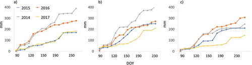
Three study areas were selected in the Kiev region: Bila Tserkva, Mironivka, and Yagotin districts (Figure 1). Agricultural fields and cultivated areas comprise more than 70% of the area in each district (“State Statistics Service of Ukraine,” n.d.). Primary crops grown in these regions are winter wheat, maize, soybean, and sunflower (Kussul et al. 2018). The agricultural production is highly associated with favorable meteorological conditions, as rainfed agriculture is predominant in these regions. In dry years, precipitation significantly reduces from 400 mm to 170 mm during the growing season (Figure 2). The majority of field crops, including grains and sunflower, are not irrigated in the study area.

Figure 1. Study areas: (a) Bila Tserkva, (b) Mironivka (c) Yahotyn districts.

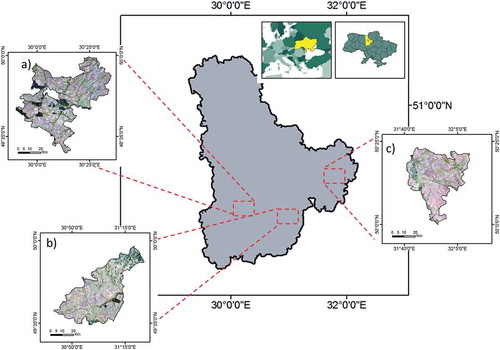
During four growing seasons, suboptimal hydrological conditions were observed in 2015 and 2017 (Figure 2). Topography in this area is mostly flat with slopes in the range of 0–2%. The soils in the area are mostly chernozems (Black soils), which are rich in organic matter and highly fertile.

Figure 2. Accumulated values of precipitation during the main crop growth period between April and September in (a) Bila Tserkva, (b) Mironivka (c) Yahotyn regions.

Data

Satellite imagery

Our analysis focused on the 2014–2017 period, which was determined by the availability of datasets encompassing consecutive growing seasons with different hydroclimatic conditions. Thirty meter Landsat-based (L8) time-series metrics that capture the seasonal variations of crops were acquired and analyzed using Google Earth Engine (GEE) cloud computing platform (Gorelick et al. 2017). The number of valid observations of optical data series might have been reduced due to poor atmospheric conditions and cloud cover. For this reason, observations from MODIS (250 m resolution) along with Landsat were integrated. This denser time-series are used to improve the quality of the output (F. Gao, Wang, and Masek 2013).

Cross-polarized Sentinel-1 C-band SAR images (S1) were also used due to their sensitivity to the attributes of a target surface such as dielectric properties and roughness (Schroeder et al. 2016). With a high spatial resolution of 5 m by 20 m (resampled to 10 m spacing for GRDH products) and a frequent revisit, S1 can be used for effective mapping and monitoring of croplands. Temporal coverage of S1 varies across the globe, but when filtering for ascending or descending mode as well as specific relative orbit, observations are available every 12 days in this particular study area. In order to test the interoperability of Sentinel-2 (S2) data with previously discussed data collections, Level-1 C (L1 C) TOA data were integrated which is also available in GEE data catalog. It provides data with high spatial resolution (10 m, 20 m, and 60 m) and frequent revisit time of 5 days at the equator under cloud-free conditions (based on constellation) and about 7–12 days in the study areas. Although the data were available for only two growing seasons, S2 imagery was still used in the analysis to test the comparability of data from different optical sensors.

Additional data

A suite of ancillary data was also compiled and used to quantitatively link crop condition and crop growth dynamics with different factors. These data sets consisted of agrometeorological observations along with land use maps. The agrometeorological data (e.g. temperature, precipitation, in-situ phenological observations) were acquired from the State Hydrometeorological Services of Ukraine for the period from 2014 to 2017 (“Ukrainian Hydrometeorological Center, Ministry of Ukraine for Emergencies ” n.d.). In addition, land use maps of the study area from 2014 to 2017 were provided by Space Research Institute (SRI) of the National Academy of Sciences of Ukraine (NASU) (Kussul et al. 2018). Additionally, in-situ observations of drought-impacted fields were acquired comprising 20 fields from 2015, 19 fields for 2017, and 14 fields from 2016 non-drought conditions from Bila Tserkva district (provided by Bila Tserkva National Agrarian University).

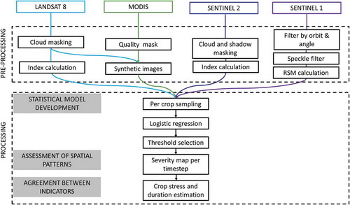
Figure 3. Workflow for drought-induced crop condition monitoring using multi-sensor data (RS stands for Remote Sensing, LST for Land Surface Temperature, RSM for Relative surface moisture).

Methods

The workflow for crop condition monitoring and estimation of drought characteristics was based on the analysis of relevant metrics derived from Sentinel-2, Landsat-8, and backscatter time-series based on Sentinel-1 (Figure 3).

Data pre-processing

To overcome the frequently missing data in Landsat time-series due to cloud cover we used MODIS and Landsat data to predict synthetic Landsat imagery for the time steps when MODIS was available. The primary selection criterion of Landsat and MODIS data pairs was their acquisition date. Both images should be acquired with the shortest temporal delay (F. Gao, Wang, and Masek 2013). With the closest pair, synthetic Landsat images were predicted based on pixel-wise linear regression (He et al. 2018). Synthetic NIR and red bands were further used for the calculation of metrics. Prior to analysis, Fmask (Function of mask) (Zhu, Wang, and Woodcock 2015) and cloud-mask flags were used for clouds and cloud shadow detection in the Landsat and MODIS imagery. For Sentinel-2 time-series we used the QA60 bitmask band which contains cloud information to mask out opaque and cirrus clouds. In addition, we used modified Temporal Dark Outlier Mask method and applied this to Sentinel-2 observations (Housman et al. 2018).

The Sentinel-1 σ₀ time-series analysis was carried out following the pre-processing of the SAR imagery. The Sentinel-1 data is available with some pre-processing applied (“Google Earth Engine API, Sentinel-1 Algorithms” n.d.) following the steps implemented in the Sentinel-1 toolbox. This pre-processing included thermal noise removal, radiometric calibration, and terrain correction. To reduce the impact of differences in viewing geometry and the orientation of the radar beam, the ascending and descending overpasses were used separately. For each location, the images were further filtered by the orbit, as the difference in orbit and incidence angles can induce changes in backscattering that are not related to geometric or dielectric properties of the target. To further reduce the effects of incidence angle variations on the backscatter, we eliminated observations with very shallow and steep incidence angles. We applied GammaMap filter to reduce speckle with the 7 × 7 kernel size (Lopes et al. 1990).

Derivation of RS parameters

Following the pre-processing of each image collection, we derived parameters based on vegetation index time-series, such as NDVI and NDMI. The latter was estimated based on NIR and SWIR (1.55–1.75 μm) (Olmos-Trujillo et al. 2020). Landsat-based NDVI was further used to derive information on the timing of green-up, senescence, and length of the growing season. These metrics were derived by estimating the DOY (day of a year) of the first NDVI observation during the growing season, which had lower/higher values than a defined threshold. Besides the aggregation of these metrics throughout the crop growth period (maximum, amplitude) as a proxy of overall condition, we studied crop condition at specific growth stages. For this, we calculated local changes of VIs within 20-day and the ratio of S1 backscatter change. For optical data, simple bi-temporal change detection was applied between before and after image acquisition time, while for SAR data change detection with the log-ratio approach was applied (R. J. Dekker 1998; Ajadi, Meyer, and Webley 2016). Taking into consideration the frequency of different observations, a 20-day interval was chosen, as this window allowed to capture changes in data acquired with all sensors (i.e. Landsat with 16-day observation, Sentinel-2 with 12-day observation). To investigate the thermal conditions of the vegetation, we used a single-channel method to derive LST based on Landsat imagery. NDVI-based surface emissivity information was used (Jimenez-Munoz and Sobrino 2010). Another metric that we investigated was the Landsat-based tasseled-cap transformation (TCT). TCT is an empirical transformation that captures critical physical characteristics of vegetation. We mainly used the wetness which is mostly linked to a combination of moisture conditions and vegetation structure. Relative surface moisture was estimated using the minimum and maximum backscatter values observed over the study period, which is considered to be equivalent to the dry reference (5th percentile) and wet reference (95th percentile) (Urban et al. 2018; Wagner, Lemoine, and Rott 1999). Thus, crop condition was described by several metrics derived from Landsat (NDVI, NDMI), the combined use of Landsat and MODIS (NDVI), Sentinel 2 and Sentinel 1 (Table 1).

Table 1. Main RS indicators tested for agricultural drought monitoring, where L8 stands for Landsat 8 observations, S2 for Sentinel 2, S1 for Sentinel-1, and L8+ MOD for Synthetic Landsat products.

Indicator	Sensor
Normalized Difference Vegetation Index	L8, S2, L8+ MOD
Normalized Difference Moisture Index	L8 ((Band 5 – Band 6)/(Band 5 + Band 6)), S2 ((Band 8 – Band 11)/(Band 8 + Band 11))
Backscatter	S1 (VH, VV)
Relative Surface Moisture	S1 (VV)
Tasseled-cap wetness	L8
Land surface temperature	L8
Phenometerics (green up, senescence, length, amplitude)	L8

Model development

We used logistic regressions to further examine crop condition and subsequent classification of drought impact in three disturbance levels based on the comparison of parameters from different conditions. In logistic regression, the probability of the outcome classes of a binary variable is modeled as a function of predictor variables. In this study, the binary outcome variable was presence (coded as 1) or absence (coded as 0) of drought. The logistic regression model was applied on sets of 20 samples for each crop in each region from their respective growing seasons. The only exception was soybean, for which the number of samples was less (28 observations less than the other crops), as in 2014, 2016, and 2017 the required number of representative fields (based on size, uniform cover) in study areas was not possible to collect. The initial drought events were identified based on historical studies and in-situ weather data. 2015 and 2017 were known to be drought years that affected large areas. Additionally, non-drought years were represented by the years 2014 and 2016 (Figure 2).

One of the challenges for the comparison of drought and non-drought conditions is the estimation of relevant thresholds that discriminate between drought and non-drought conditions, as well as varying levels of drought impact level, namely low, moderate, and severe as they can be different among different crop types, locations, and seasons. Typically, a relative VI value or a deviation of a VI value from a baseline is used as an indicator of drought. Crop rotations in the study area and related year to year changes in crop type made a comparison of indicators based on optical and SAR data difficult. Instead of deriving these indicators from different years at the same location, we compared the condition of the respective crop from different locations in different years. The output of the logistic regression was used to evaluate the drought-induced variability of remotely sensed parameters. The variables with the highest prediction rate were further used to estimate the thresholds for drought/non-drought classification. The models were evaluated using the area under the receiver operating characteristic (ROC) curve (AUC). AUC is a performance measure that considers all classification thresholds and shows if the probability of drought versus non-drought condition was correctly estimated by the logistic model (Powers 2011). The AUC ranges in values between 0 (model with wrong predictions) and 1 (model with perfect predictive ability). For each variable which yielded in a statistically significant result (p < 0.05) and satisfactory prediction accuracy, we derived a value at which the parameter discriminated drought and non-drought conditions. Based on these values, crop-specific thresholds for three levels were subsequently estimated. Using the binary drought/non-drought information derived for each time step, the length of drought was estimated based on the consecutive occurrence of drought for at least two timesteps. We validated the results derived from different parameters with the in-situ field data (53 fields in total) from 2015 to 2017. Finally, the agreement of outputs based on the different sensors was estimated. For this, the rasters for each timestep were resampled to the same resolution (30 m). Then, an array representing the drought/non-drought condition was created for each pixel. The total number of instances of drought in each array was calculated.

Results and discussion

Comparing the parameters extracted from different sensors

Remotely sensed time-series were used to derive indicators from a single data source (Landsat, Sentinel-1, and Sentinel-2) or fused series (Landsat/MODIS) and to assess drought-induced properties during 2014–2017. Among the variables tested in this study, NDMI, LST, and SAR-based relative moisture index had a significant impact on the prediction of drought occurrence. The accuracy of different models varied based on region, crop of interest, and remotely sensed derivatives.

In general, within all models, maize was affected the most compared to other crops. This can be explained by the fact that crops are characterized by a different sensitivity to water-deficiency (Zhang et al. 2017). NDVI and NDMI from different sensors exhibited similar results (i.e. AUC, prediction rate) for positive and negative predictions when applying the logistic model. Particularly, NDVI and NDMI accuracies ranged between 50% and 70% and 52 and 75%, respectively. These results are in line with other studies and can be explained with the properties of SWIR that reflect changes in water content. The lowest accuracies were observed for soybean, with an AUC value of 0.57 due to a lower number of samples.

The MODIS/Landsat-based methods were less accurate compared to results derived from Sentinel 2 and Landsat. One possible explanation is the higher intrapixel heterogeneity at the MODIS scale, which results in an underestimation of drought impact. As a result, best MODIS/Landsat-based models produced satisfactory results, with an AUC value of 0.72.

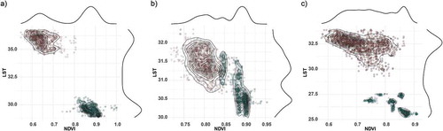
Local parameters (e.g. short-term maximum, amplitude within a month) describing within seasonal changes, especially those from mid growth period, were sensitive to drought as well. The only constraint for this was the decreasing number of samples, due to masked values in the optical data set. LST was significantly higher for crops under unfavorable conditions during mid-season of 2017. This was observed for maize and sunflower with the highest AUC values 0.86 and 0.79, respectively. As a result, all drought-affected fields could be discriminated (Figure 4). This is in agreement with several studies reporting that the period around anthesis is particularly sensitive to heat stress in nearly all crops (Luo 2011). The link between vegetation indices and LST is attributed to changes in the proportion of vegetation cover and moisture conditions, showing that surface temperature may quickly increase with drought stress (Johnson 2014).

Figure 4. NDVI/LST density plots for (a) maize, (b) soybean and (c) sunflower during the mid-growing season in 2017 (red) and 2016 (green) derived from Landsat-8.

Although differences in the length of the growing season were observed among drought and non-drought years, they were not statistically significant. Furthermore, tasseled cap wetness did not yield statistically significant results and so this was not used for further analysis. Including SAR input variables into the logistic model resulted in satisfactory performance with an AUC value of 0.65 and an accuracy of 60% only for maize. Best results were acquired from observations during the tasseling and silking period.

Temporal variability of RS metrics during drought and non-drought years

Two major drought occurrences differing in intensity, timing, duration, and location were examined over the three study sites in Ukraine between 2014 and 2017. The results of this study illustrate that optical time-series, including NDVI, MDMI, play a primary role in determining drought occurrence.

Figure 5. Time-series of NDVI derived from optical sensors for (a) Maize, (b) Sunflower, (c) Soy, (d) Wheat with blue depicting non-drought conditions (2016) and black drought conditions (2017).

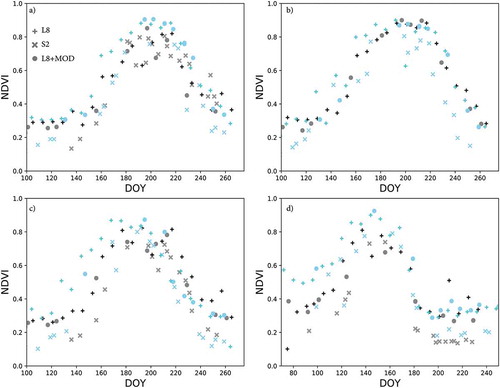
The most pronounced and significant changes were observed during the peak growing season and corresponded to anthesis and ripening stages of summer crops (Figure 5). The NDVI derived from different sensors, in general, was similar for both drought and non-drought conditions. The local amplitudes of NDVI were high in drought-affected fields reaching a value of 0.4. When using the SAR backscattering signal, higher fluctuations of intensity in drought-affected fields of maize were observed. For the other crops, the backscattering intensity was highly variable. This was most prominent for wheat. Particularly, lower backscatter during the non-drought condition was observed, which can be caused by increased attenuation. Backscattering intensity is a function of the geometry and the dielectric properties of a crop. As crop height and water content are changing throughout the growing season, it is generally difficult to decompose drought factors. Crops’ growth period is visible as an increase in reflectivity in the VH band (Figure 6). Backscatter generally increases as water content in vegetation increases. Similarly, backscatter intensity decreases with the decline of wet biomass, which could be observed in this study at the end of the growing season.

Figure 6. Time-series of backscattering coefficient for (a) Maize, (b) Sunflower, (c) Soy, (d) Wheat with blue depicting non-drought conditions (2016) and black drought conditions (2017).

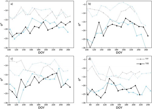
The sensitivity of VV backscatter to soil moisture in maize (Figure 6a) can be explained by larger row spacing on maize fields. Because of this, bare soil remains visible until far in late spring and so VV backscatter is not attenuated by vegetation and can be still affected by soil moisture. Similar results have been reported by other studies (Vreugdenhil et al. 2018).

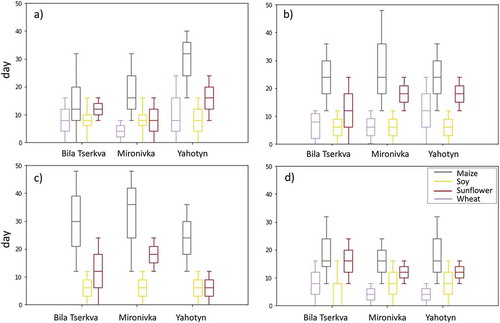
In this study, the maximum drought duration identified varied among different drought indicators (Figure 7). Based on our analysis, the maximum drought duration appeared to be higher in the SAR-based variables than in the optical indices. Maize was the most sensitive to a drought of 1 month occurring in July, which corresponds with silking and early reproductive stages. This agrees with other studies, where NDVI was evaluated for maize response to drought (R. Wang et al. 2016). For wheat, we observed high sensitivity, particularly in June. These results are in line with agricultural statistics and coarse resolution analysis based on FAO Agricultural Stress index (FAO, GIEWS Agricultural Stress Index, 2018). Even though large areas of wheat with suboptimal conditions were observed in 2015 especially in Bila Tserkva region, this was not reflected in the yield statistics which did not depict drastic yield decrease. This might be explained by the recovery of the crop due to sufficient rainfall and optimal thermal conditions during the subsequent stages of crop growth following the deficit of precipitation at the end of May and the start of June. For further understanding of the winter wheat response to drought hazard, the study of conditions during the winter months is still needed.

One of the limiting factors for the estimation of drought duration was the temporal frequency of remotely sensed observations. This was critical for cases when periods of precipitation deficit were shorter than the revisit time of the sensor. As a result, drought-induced changes were not fully depicted by the indicator.

Figure 7. Length of the drought estimated in 2017 from (a) Landsat NDMI (b) Sentinel 2 NDMI, (c) Sentinel 1, (d) L8+ MOD NDVI.

The results from the present study indicate, that VIs were not sensitive to drought stress at early growth stages. Although considered as moderately drought tolerant, we observed drought impacts on sunflower fields in three regions.

In general, derivatives from optical sensors reported similar timing of the start of drought. On the contrary, SAR derived onset of crop stress appeared 12–24 days earlier than those derived from optical data. Coupled with the declined precipitation during the growing season as well as reduced crop yields, this indicates that drought-induced properties of time-series can be characterized based on temporal metrics. Temporal features showed that different crops experience different intensities of drought impact (Figure 8). Moreover, the described drought-induced properties were more prevailing in different regions of the study, as opposed to local management differences, which would be allocated to specific smaller areas.

Spatial distribution of drought impact

For each of the identified drought events, the corresponding areas being affected by recurrent drought were mapped. The results identified areas that were affected by drought when using different indicators for different crops ranging from 20% (for soybean) to 44% (maize) in 2017. In general, areas affected by drought varied for different crops. We observed the highest affected areas for maize, for both 2015 and 2017, whereas the areas for other summer crops (sunflower and soy) comprised 23–30% of the cultivated area. These estimates were different compared to the tests on non-drought years, where areas under sub-optimal conditions were less than 10%. The only exception was soybean, in which approximately 16% of the cultivated area under severe, moderate, and mild stress were observed, although the year of 2016 exhibited more favorable conditions. Depiction of these false-positive stressed areas can be caused by different management practices and cultivar change which were not examined in this study.

Figure 8. Spatially explicit drought mapping series based on Landsat time-series in June, July, and August during two sub-optimal growing seasons (a)-(c) in 2015 and (d)-(f) in 2017.

The drought-impacted areas as derived from remotely sensed crop condition variables also differed with time (Figure 8). In the case of 2015, we identified larger affected areas at the end of the growing season, whereas in 2017, the drought impact could be observed at earlier stages of the growing season. For summer crops, the drought impact could be observed during mid-growing season in 2017. Specifically, the distribution of the drought-impacted fields based on different data such as NDMI is illustrated, which reached high accuracies of up to 75% for maize (Figure 9). Based on optical data, drought-impacted fields of different crops can generally be identified. In the case of relative surface moisture derived from Sentinel 1, accurate results were achieved in this study only for maize.

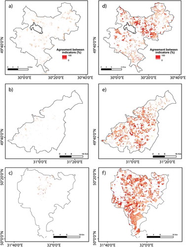
The agreement maps based on peak growing season (July) for maize show that in the majority of the fields, the indicators exhibited more than 50% agreement for 2017. This shows that data from different sensors indicate a similar condition for the crop and are comparable, and thus further integration of the datasets is feasible (Figure 10). Whereas for 2015, both the detected drought-impacted fields and the pixel-based percentage agreement between five indicators are lower, which can be due to the later onset of the drought.

The major environmental drivers that affected crop productivity were used to assess the results of the study. Firstly, we checked the total precipitation during the critical stages throughout the growing season (April–August) which was 50–180 mm less. However, precipitation was not evenly distributed during the growing season, and there were periods without rain during start-mid July.

Examination of several crops showed that in different regions of the study area yields decreased significantly in 2017 relative to the years with no drought condition. Mainly, for soybean, a 26–30% decrease was recorded and sunflower yields were 17–26% less, whereas maize and wheat yields decreased by 16–40% and 20–33%, respectively. The yield losses, in general, were less in 2015, especially for wheat and sunflower comprising 7–10% compared to non-drought years. Nevertheless, in 2015 maize and soy had a 20% yield decrease.

Figure 9. Drought-impacted crops in 2017 derived from (a)-(c) Sentinel 1 based Relative Surface Moisture and (d)-(f) Sentinel 2 based NDMI during the peak of the growing season (July).

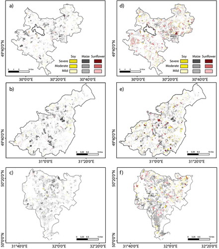
Figure 10. Percentage agreement between different indicators (a)-(c) in July 2015 (LST, S1, L8 NDMI, L8 NDVI, MOD+L8 NDVI) and (d)-(f) 2017 (LST, S1, L8 NDMI, S2 NDMI, MOD+L8 NDVI).

Potentials and limitations of the proposed approach

Although the results of the logistic model show sufficient accuracy (~70%) and the number of estimated drought-impacted fields was in good agreement with field data (correct allocation in drought/non-drought class for 75% of the fields with optical data), there is still need for larger validation datasets. Furthermore, certain factors may have contributed to some uncertainties in the estimates of drought impact and its timing. In general, agricultural land cover is characterized by substantial variations within relatively short time intervals. Even though some of these variations might have been caused by agricultural practices (e.g. individual irrigation not reflected in the statistics, fertilizer use), plant disease, cultivar change, the study allowed to detect drought-induced changes in crop condition. Another issue is the integration of parameters such as soil moisture which would be verified based on in-situ measurements. Furthermore, the temporal granularity of remotely sensed data can affect the accuracy of the estimated duration of drought. Especially with optical data, cloud cover can reduce the number of images applicable in the time-series. Further fusion of the datasets, such as Sentinel 2 integration with Landsat, can significantly increase the temporal frequency of data for dense time-series analyses (Chastain et al. 2019; Claverie 2015). Calibration of models and evapotranspiration derivation, as well as integration of different combined indices such as Temperature Vegetation Dryness Index (TVDI) (Z. Gao, Gao, and Chang 2011), Normalized Multi-band Drought Index (NMDI) (L. Wang and Qu 2007) can further improve large-scale monitoring and understanding of vegetation stress and overall dynamics during the growing season.

Nevertheless, our results contribute to the general understanding of climate-induced variations in crop condition by quantifying spatial and temporal variability in drought for major crops in three study areas. Considering that the study was conducted in a real environment instead of controlled field experiments, as well as assuming the uncertainties, such as cloud cover, this study highlights the feasibility of crop condition monitoring at a farm management scale in a wider range of environmental conditions and scales. Such understanding of spatio-temporal variability makes it possible to identify both trends: where and when drought-induced properties can be observed with satellite remote sensing, and how sensitivity to drought has evolved over time. This may help mitigate drought response at field, county, state, and national levels. In the present study, approximately 45% of the cropping areas were associated with sub-optimal growing condition in the key stages of crop phenology and growth. The results of the study may be used to further develop agricultural management strategies that help mitigating impacts of drought on agricultural production, especially at larger spatial scales.

Conclusions

The current study introduces new sets of parameters for crop condition monitoring and thereby demonstrates the potential of optical and SAR data to assess crop conditions at spatial scales that can support decision-making even beyond fields and farms. The combined use of RS data from SAR and multispectral Sentinel-2, together with Landsat and lower resolution MODIS time-series, provides opportunities for promising applications in crop monitoring. It especially allows the derivation of crop variables that indicate sensitivity to drought-related stress in croplands. Derived drought-induced crop condition is influenced by crop type and the timing of the drought. The findings show that moisture index, SAR backscatter, and land surface temperature could explain drought occurrence and impact level in crops. These dense time-series can be further used for crop water use estimation and near real-time crop water requirement estimation. The advancement of large area soil moisture and evapotranspiration estimation and the use of harmonized Landsat and Sentinel-2 time-series can further improve operational crop water management. The applicability of the method can be further investigated by upscaling and applying it over larger areas as well as testing it on other crops. The methods demonstrated here can be applied to areas requiring early warning of food shortage or improved agricultural monitoring to ensure greater sustainability within the agriculture sector.

Acknowledgements

We thank Tatyana Adamenko and Grygoriy Melnik for their support with in-situ data collection. We are grateful to Guido Lüchters for his help with the statistical analysis. 

Disclosure statement

No potential conflict of interest was reported by the authors.

Funding

The research support was provided by the German Federal Ministry of Education and Research (Project: GlobeDrought, grant no. 02WGR1457F BMBF Project ID: 02WGR1457A-F).

Data availability statement

The raw imagery is available from the Google Earth Engine data catalog (https://developers.google.com/earth-engine/datasets) (Landsat 8 Surface Reflectance, MOD09Q1.006 Terra Surface Reflectance, Sentinel-2 MSI, Sentinel-1 SAR GRD). Sharing of supporting in-situ datasets is subject to third party permission. They may be available on request providing permission is granted by the corresponding organizations.

References

- Adamenko, T., and A. Prokopenko. 2011. “Monitoring Droughts and Impacts on Crop Yield in Ukraine from Weather and Satellite Data.” In Use of Satellite and In-Situ Data to Improve Sustainability, edited by F. Kogan, A. Powell, and O. Fedorov, 3–9. Springer Netherlands: NATO Science for Peace and Security Series C: Environmental Security. doi:10.1007/978-90-481-9618-0_1.
- AghaKouchak, A., A. Farahmand, F. S. Melton, J. Teixeira, M. C. Anderson, B. D. Wardlow, and C. R. Hain. 2015. “Remote Sensing of Drought: Progress, Challenges and Opportunities.” Reviews of Geophysics 53 (2): 2014RG000456. doi:10.1002/2014RG000456.
- Ahmadalipour, A., H. Moradkhani, H. Yan, and M. Zarekarizi. 2017. “Remote Sensing of Drought: Vegetation, Soil Moisture, and Data Assimilation.” In Remote Sensing of Hydrological Extremes, edited by V. Lakshmi, 121–149. Springer Remote Sensing/Photogrammetry. Cham: Springer International Publishing. doi:10.1007/978-3-319-43744-6_7.
- Ajadi, O. A., F. J. Meyer, and P. W. Webley. 2016. “Change Detection in Synthetic Aperture Radar Images Using a Multiscale-Driven Approach.” Remote Sensing 8 (6): 482. doi:10.3390/rs8060482.
- Bhuiyan, C., A. K. Saha, N. Bandyopadhyay, and F. N. Kogan. 2017. “Analyzing the Impact of Thermal Stress on Vegetation Health and Agricultural Drought – A Case Study from Gujarat, India.” GIScience & Remote Sensing 54 (5): 678–699. doi:10.1080/15481603.2017.1309737.
- Bolten, J. D., W. T. Crow, X. Zhan, T. J. Jackson, and C. A. Reynolds. 2010. “Evaluating the Utility of Remotely Sensed Soil Moisture Retrievals for Operational Agricultural Drought Monitoring.” IEEE Journal of Selected Topics in Applied Earth Observations and Remote Sensing 3 (1): 57–66. doi:10.1109/JSTARS.2009.2037163.
- Chastain, R., I. Housman, J. Goldstein, and M. Finco. 2019. “Empirical Cross Sensor Comparison of Sentinel-2A and 2B MSI, Landsat-8 OLI, and Landsat-7 ETM+ Top of Atmosphere Spectral Characteristics over the Conterminous United States.” Remote Sensing of Environment 221 (February): 274–285. doi:10.1016/j.rse.2018.11.012.
- Chen, D., J. Huang, and T. J. Jackson. 2005. “Vegetation Water Content Estimation for Corn and Soybeans Using Spectral Indices Derived from MODIS Near- and Short-Wave Infrared Bands.” Remote Sensing of Environment 98 (2): 225–236. doi:10.1016/j.rse.2005.07.008.
- Claverie, M. 2015. “A Harmonized Landsat-Sentinel-2 Surface Reflectance Product: A Resource for Agricultural Monitoring.” In. Agu. https://agu.confex.com/agu/fm15/webprogram/Paper85646.html
- Dekker, R. J. 1998. “Speckle Filtering in Satellite SAR Change Detection Imagery.” International Journal of Remote Sensing 19 (6): 1133–1146. doi:10.1080/014311698215649.
- Enenkel, M., C. Steiner, T. Mistelbauer, W. Dorigo, W. Wagner, L. See, C. Atzberger, S. Schneider, and E. Rogenhofer. 2016. “A Combined Satellite-Derived Drought Indicator to Support Humanitarian Aid Organizations.” Remote Sensing 8 (4): 340. doi:10.3390/rs8040340.
- n.d. “FAO,GIEWS, Earth Observation,Seasonal Global Indicators,METOP, NDVI, ASIS, VHI, VCI,ECWMF, Agricultural Stress Index, NDVI Anomaly,Vegetation Condition Index,Vegetation Health Index,Estimated Precipitation,Precipitation AnomalyMap.” Accessed 10 November 2018. http://www.fao.org/giews/earthobservation/asis/index_1.jsp?lang=en
- Gao, F., P. Wang, and J. Masek. 2013. “Integrating Remote Sensing Data from Multiple Optical Sensors for Ecological and Crop Condition Monitoring.” In, 8869: 886903-886903–8. https://doi.10.1117/12.2023417
- Gao, Z., W. Gao, and N.-B. Chang. 2011. “Integrating Temperature Vegetation Dryness Index (TVDI) and Regional Water Stress Index (RWSI) for Drought Assessment with the Aid of LANDSAT TM/ETM+ Images.” International Journal of Applied Earth Observation and Geoinformation 13 (3): 495–503. doi:10.1016/j.jag.2010.10.005.
- Google Earth Engine API, Sentinel-1 Algorithms. n.d. “Google Developers.” Accessed 9 November 2018. https://developers.google.com/earth-engine/sentinel1
- Gorelick, N., M. Hancher, M. Dixon, S. Ilyushchenko, D. Thau, and R. Moore. 2017. “Google Earth Engine: Planetary-Scale Geospatial Analysis for Everyone.” Remote Sensing of Environment 202: 18–27. doi:10.1016/j.rse.2017.06.031.
- Gu, Y., J. F. Brown, J. P. Verdin, and B. Wardlow. 2007. “A Five-Year Analysis of MODIS NDVI and NDWI for Grassland Drought Assessment over the Central Great Plains of the United States.” Geophysical Research Letters 34 (6). doi:10.1029/2006GL029127.
- Guttman, N. B. 1998. “Comparing the Palmer Drought Index and the Standardized Precipitation Index1.” JAWRA Journal of the American Water Resources Association 34 (1): 113–121. doi:10.1111/j.1752-1688.1998.tb05964.x.
- He, M., J. Kimball, M. Maneta, B. Maxwell, A. Moreno, S. Beguería, X. Wu, et al. 2018. “Regional Crop Gross Primary Productivity and Yield Estimation Using Fused Landsat-MODIS Data.” Remote Sensing 10 (3): 372. doi:10.3390/rs10030372.
- Housman, I., R. Chastain, M. Finco, I. W. Housman, R. A. Chastain, and M. V. Finco. 2018. “An Evaluation of Forest Health Insect and Disease Survey Data and Satellite-Based Remote Sensing Forest Change Detection Methods: Case Studies in the United States.” Remote Sensing 10 (8): 1184. doi:10.3390/rs10081184.
- Ivits, E., S. Horion, R. Fensholt, and M. Cherlet. 2014. “Drought Footprint on European Ecosystems between 1999 and 2010 Assessed by Remotely Sensed Vegetation Phenology and Productivity.” Global Change Biology 20 (2): 581–593. doi:10.1111/gcb.12393.
- Ji, L., L. Zhang, B. K. Wylie, and J. Rover. 2011. “On the Terminology of the Spectral Vegetation Index (NIR − SWIR)/(NIR + SWIR).” International Journal of Remote Sensing 32 (21): 6901–6909. doi:10.1080/01431161.2010.510811.
- Jimenez-Munoz, J. C., and J. A. Sobrino. 2010. “A Single-Channel Algorithm for Land-Surface Temperature Retrieval from ASTER Data.” IEEE Geoscience and Remote Sensing Letters 7 (1): 176–179. doi:10.1109/LGRS.2009.2029534.
- Johnson, D. M. 2014. “An Assessment of Pre- and within-Season Remotely Sensed Variables for Forecasting Corn and Soybean Yields in the United States.” Remote Sensing of Environment 141 (February): 116–128. doi:10.1016/j.rse.2013.10.027.
- Karnieli, A., R. T. Nurit Agam, M. A. Pinker, M. L. Imhoff, G. G. Gutman, N. Panov, and A. Goldberg. 2010. “Use of NDVI and Land Surface Temperature for Drought Assessment: Merits and Limitations.” Journal of Climate 23 (3): 618–633. doi:10.1175/2009JCLI2900.1.
- Klisch, A., and C. Atzberger. 2016. “Operational Drought Monitoring in Kenya Using MODIS NDVI Time Series.” Remote Sensing 8 (4): 267. doi:10.3390/rs8040267.
- Kogan, F. 2018. Remote Sensing for Food Security. Cham: Springer International Publishing.
- Kogan, F., T. Adamenko, and W. Guo. 2013. “Global and Regional Drought Dynamics in the Climate Warming Era.” Remote Sensing Letters 4 (4): 364–372. doi:10.1080/2150704X.2012.736033.
- Kussul, N., L. Mykola, A. Shelestov, and S. Skakun. 2018. “Crop Inventory at Regional Scale in Ukraine: Developing in Season and End of Season Crop Maps with Multi-Temporal Optical and SAR Satellite Imagery.” European Journal of Remote Sensing 51 (1): 627–636. doi:10.1080/22797254.2018.1454265.
- Lopes, A., E. Nezry, R. Touzi, and H. Laur. 1990. “Maximum A Posteriori Speckle Filtering And First Order Texture Models In Sar Images.” In 10th Annual International Symposium on Geoscience and Remote Sensing, 2409–2412, College Park, Maryland, USA. https://doi.10.1109/IGARSS.1990.689026
- Luo, Q. 2011. “Temperature Thresholds and Crop Production: A Review.” Climatic Change 109 (3): 583–598. doi:10.1007/s10584-011-0028-6.
- Mishra, A. K., A. V. M. Ines, N. N. Das, C. P. Khedun, V. P. Singh, B. Sivakumar, and J. W. Hansen. 2015. “Anatomy of a Local-Scale Drought: Application of Assimilated Remote Sensing Products, Crop Model, and Statistical Methods to an Agricultural Drought Study.” Journal of Hydrology, Drought Processes, Modeling, and Mitigation 526 (July): 15–29. doi:10.1016/j.jhydrol.2014.10.038.
- Moran, M. S., L. Alonso, J. F. Moreno, M. P. Cendrero Mateo, D. F. de la Cruz, and A. Montoro. 2012. “A RADARSAT-2 Quad-Polarized Time Series for Monitoring Crop and Soil Conditions in Barrax, Spain.” IEEE Transactions on Geoscience and Remote Sensing 50 (4): 1057–1070. doi:10.1109/TGRS.2011.2166080.
- Olmos-Trujillo, E., J. González-Trinidad, H. Júnez-Ferreira, A. Pacheco-Guerrero, C. Bautista-Capetillo, C. Avila-Sandoval, and E. Galván-Tejada. 2020. “Spatio-Temporal Response of Vegetation Indices to Rainfall and Temperature in A Semiarid Region.” Sustainability 12 (5): 1939. doi:10.3390/su12051939.
- Palmer, W. 1965. “Meteorological Drought.” US. Weather Bureau Res. Paper, no. 45, 1–58.
- Patel, N. R., P. Chopra, and V. K. Dadhwal. 2007. “Analyzing Spatial Patterns of Meteorological Drought Using Standardized Precipitation Index.” Meteorological Applications 14 (4): 329–336. doi:10.1002/met.33.
- Peng, C., L. Di, M. Deng, W. Han, and A. Yagci. 2013. “A Comprehensive Agricultural Drought Stress Monitoring Method Integrating MODIS and Weather Data (A Case Study of Iowa).” In 2013 Second International Conference on Agro-Geoinformatics (Agro-Geoinformatics), 147–152, Fairfax, VA, USA. https://doi.10.1109/Argo-Geoinformatics.2013.6621898
- Powers, D. M. 2011. “Evaluation: From Precision, Recall and F-Measure to ROC, Informedness, Markedness and Correlation.”
- Rao, M., Z. Silber-Coats, S. Powers, L. Fox III, and A. Ghulam. 2017. “Mapping Drought-Impacted Vegetation Stress in California Using Remote Sensing.” GIScience & Remote Sensing 54 (2): 185–201. doi:10.1080/15481603.2017.1287397.
- Sadegh, M., C. Love, A. Farahmand, A. Mehran, M. J. Tourian, and A. AghaKouchak. 2017. “Multi-Sensor Remote Sensing of Drought from Space.” In Remote Sensing of Hydrological Extremes, edited by V. Lakshmi, 219–247. Springer Remote Sensing/Photogrammetry. Cham: Springer International Publishing. doi:10.1007/978-3-319-43744-6_11.
- Schroeder, R., K. C. McDonald, M. Azarderakhsh, and R. Zimmermann. 2016. “ASCAT MetOp-A Diurnal Backscatter Observations of Recent Vegetation Drought Patterns over the Contiguous U.S.: An Assessment of Spatial Extent and Relationship with Precipitation and Crop Yield.” Remote Sensing of Environment 177 (May): 153–159. doi:10.1016/j.rse.2016.01.008.
- Skakun, S., N. Kussul, A. Shelestov, and O. Kussul. 2015. “The Use of Satellite Data for Agriculture Drought Risk Quantification in Ukraine.” Geomatics, Natural Hazards and Risk: 1–18. doi:10.1080/19475705.2015.1016555.
- State Statistics Service of Ukraine. n.d. Accessed 19 October 2018. http://www.ukrstat.gov.ua/
- Tadesse, T., C. Champagne, B. D. Wardlow, T. A. Hadwen, J. F. Brown, G. B. Demisse, Y. A. Bayissa, and A. M. Davidson. 2017. “Building the Vegetation Drought Response Index for Canada (Vegdri-canada) to Monitor Agricultural Drought: First Results.” GIScience & Remote Sensing 54 (2): 230–257. doi:10.1080/15481603.2017.1286728.
- Ukrainian Hydrometeorological Center,Ministry of Ukraine for Emergencies. n.d. Accessed 27 April 2020. https://meteo.gov.ua/en/33345/hmc/hmc_main/,01030,Kyiv,str.Zolotovoritska,6-B
- Urban, M., C. Berger, T. Mudau, K. Heckel, J. Truckenbrodt, V. O. Odipo, I. Smit, et al. 2018. “Surface Moisture and Vegetation Cover Analysis for Drought Monitoring in the Southern Kruger National Park Using Sentinel-1, Sentinel-2, and Landsat-8.” Remote Sensing 10 (9): 1482. doi:10.3390/rs10091482.
- van Hoek, M., L. Jia, J. Zhou, C. Zheng, and M. Menenti. 2016. “Early Drought Detection by Spectral Analysis of Satellite Time Series of Precipitation and Normalized Difference Vegetation Index (NDVI).” Remote Sensing 8 (5): 422. doi:10.3390/rs8050422.
- Veloso, A., S. Mermoz, A. Bouvet, T. Le Toan, M. Planells, J.-F. Dejoux, and E. Ceschia. 2017. “Understanding the Temporal Behavior of Crops Using Sentinel-1 and Sentinel-2-like Data for Agricultural Applications.” Remote Sensing of Environment 199 (September): 415–426. doi:10.1016/j.rse.2017.07.015.
- Vicente-Serrano, S. M., S. Beguería, and J. I. López-Moreno. 2009. “A Multiscalar Drought Index Sensitive to Global Warming: The Standardized Precipitation Evapotranspiration Index.” Journal of Climate 23 (7): 1696–1718. doi:10.1175/2009JCLI2909.1.
- Vreugdenhil, M., W. Wagner, B. Bauer-Marschallinger, I. Pfeil, I. Teubner, C. Rüdiger, and P. Strauss. 2018. “Sensitivity of Sentinel-1 Backscatter to Vegetation Dynamics: An Austrian Case Study.” Remote Sensing 10 (9): 1396. doi:10.3390/rs10091396.
- Wagner, W., G. Lemoine, and H. Rott. 1999. “A Method for Estimating Soil Moisture from ERS Scatterometer and Soil Data.” Remote Sensing of Environment 70 (2): 191–207. doi:10.1016/S0034-4257(99)00036-X.
- Wang, L., and J. J. Qu. 2007. “NMDI: A Normalized Multi-Band Drought Index for Monitoring Soil and Vegetation Moisture with Satellite Remote Sensing.” Geophysical Research Letters 34 (20). doi:10.1029/2007GL031021.
- Wang, R., K. Cherkauer, L. Bowling, R. Wang, K. Cherkauer, and L. Bowling. 2016. “Corn Response to Climate Stress Detected with Satellite-Based NDVI Time Series.” Remote Sensing 8 (4): 269. doi:10.3390/rs8040269.
- Wardlow, B. D., M. C. Anderson, and J. P. Verdin. 2012. Remote Sensing of Drought: Innovative Monitoring Approaches. Boca Raton: CRC Press.
- Wu, D., J. J. Qu, and X. Hao. 2015. “Agricultural Drought Monitoring Using MODIS-Based Drought Indices over the USA Corn Belt.” International Journal of Remote Sensing 36 (21): 5403–5425. doi:10.1080/01431161.2015.1093190.
- Zargar, A., R. Sadiq, B. Naser, and F. I. Khan. 2011. “A Review of Drought Indices.” Environmental Reviews 19 (NA): 333–349. doi:10.1139/a11-013.
- Zhang, X., N. Chen, J. Li, Z. Chen, and D. Niyogi. 2017. “Multi-Sensor Integrated Framework and Index for Agricultural Drought Monitoring.” Remote Sensing of Environment 188 (January): 141–163. doi:10.1016/j.rse.2016.10.045.
- Zhu, Z., S. Wang, and C. E. Woodcock. 2015. “Improvement and Expansion of the Fmask Algorithm: Cloud, Cloud Shadow, and Snow Detection for Landsats 4–7, 8, and Sentinel 2 Images.” Remote Sensing of Environment 159 (March): 269–277. doi:10.1016/j.rse.2014.12.014.