Analyzing ice dynamics using Sentinel-1 data at the Solheimajoküll Glacier, Iceland

ABSTRACT

The climate in southern Iceland has warmed over the last 70 years, resulting in accelerated glacier dynamics at the Solheimajoküll glacier. In this study, we compare glacier terminus locations from 1973 to 2018, to changes in climate across the study area, and we derive ice-surface velocities (2015–2018) from satellite remote-sensing imagery (Sentinel-1) using the offset-tracking method. There have been two regional temperature trends in the study period: cooling (1973–1979) and warming (1980–2018). Our results indicate a time lag of about 20 years between the onset of glacier retreat (−53 m/year since 2000) and the inception of the warming period. Seasonally, the velocity time series suggest acceleration during the summer melt season since 2016, whereas glacier velocities during accumulation months were constant. The highest velocities were observed at high elevations where the ice-surface slope is the steepest. We tested several scenarios to assess the hydrological time response to glacier accelerations, with the highest correlations being found between one and 30 days after the velocity estimates. Monthly correlation analyses indicated inter-annual and intra-annual variability in the glacier dynamics. Additionally, we investigate the linkage between glacier velocities and meltwater outflow parameters as they provide useful information about internal processes in the glacier. Velocity estimates positively correlate with water level and negatively correlate with water conductivity between April and August. There is also a disruption in the correlation trend between water conductivity and ice velocity in June, potentially due to a seasonal release of geothermal water.

KEYWORDS:

• Climate conditions
• glacier velocity
• offset-tracking method
• Sentinel-1
• remote sensing

1. Introduction

Satellite remote sensing is a cost-effective tool for monitoring global climate and related impacts (Rose et al. 2015). Satellite data effectively monitor inaccessible areas, capturing events such as glacier surges (De Angelis and Skvarca 2003), enabling delimitation of wet snow from glacier ice (Nesje and Dahl 2016; Ryan et al. 2019), mapping ice-flow velocity (Kraaijenbrink et al. 2016) and the retreat/advance of glacier termini (Sigurđsson, Jónsson, and Jóhannesson 2007). Despite the capacity of optical imagery to monitor glaciers (Racoviteanu, Williams, and Barry 2008), the presence of clouds is a notable limitation (Eberhardt et al. 2016). Satellites with Synthetic Aperture Radar (SAR) sensors are therefore important for monitoring the cryosphere (Bermudez et al. 2018) because they are not reliant on solar illumination and are quite independent of weather conditions (Bermudez et al. 2018). Thus, SAR imagery is particularly beneficial where optical image availability is limited by cloud cover and/or polar night (Winsvold et al. 2018). Sentinel-1A and Sentinel-1B satellites were launched (2014 and 2016, respectively) to continue with ESA´s Earth observation program using SAR methods (Mattar et al. 1998; Rott, Rack, and Nagler 2007; Erten et al. 2009; Yasuda and Furuya 2013). Sentinel-1 satellites enhance key characteristics of previous ESA-SAR satellites (ERS and Envisat) in terms of data reliability, revisit time and geographic coverage (Torres et al. 2012).

Glacier advance or retreat depend on mass balance, which is impacted by climate (Dowdeswell et al. 1997). According to Anderson et al. (2019), about 11% of Iceland is covered by glaciers (~ 3600 km³ of ice). If all this ice melted, the mean sea level would rise by ~ 1 cm (Björnsson and Pálsson 2008; Björnsson et al. 2013). The Icelandic ablation season typically lasts three to 4 months (June to mid-September). During this period, the most important factors that affect glacier mass balance are solar radiation and air temperature (Houghton 2004), whereas precipitation is the most important factor during the accumulation season (October to May). Other factors may also alter the mass balance of glaciers, including geothermal or volcanic activity, debris on the glacier surface, and calving (Sigurđsson, Jónsson, and Jóhannesson 2007). In Iceland, a negative mass balance has been reported since 1997 for most non-surge type glaciers, which has resulted in glacier terminus retreat. This coincides with climate shifts where the rate of advance or retreat of glaciers is accompanied by delays of a few years (Sigurđsson, Jónsson, and Jóhannesson 2007). Continued climate warming accelerates runoff from Iceland´s glaciers while many glaciers are forecast to nearly disappear over the next 100–200 years (Jóhannesson et al. 2004; Björnsson 2017).

The Solheimajoküll glacier has one of the longest and most glacier fluctuation records in Iceland (Staines et al. 2015). Jaenicke et al. (2006) observed correlation between annual mean air temperature and glacier mass balance at this glacier, indicating negative mass-balance as mean air-temperature increases. Some estimations suggest an overall volume loss of 18.9 ± 1.6 km³ (~55 km²) for the entire Mýrdalsjökull ice cap between 1960 and 2010 (Gunnlaugsson et al. 2016). In this context, ice-surface lowering for Solheimajoküll would be about 10–15 m height between 1960 and 2010, while neighboring outlets such as Klifurárjökull and Goðalandsjökull have lost up to 120 m of elevation at their margins (Gunnlaugsson et al. 2016). In July 1953, Eyþórsson et al. (1953) carried out one of the first in-situ measurements of ice velocities at Solheimajoküll, recording values from 0.56 to 1.24 m/day during the ablation period. A more recent study found that surface velocities were ≤ 0.2 m for a time period of 73 days (between 30^th April and 11 July 2013) (James, How, and Wynn 2016). Furthermore, they detected a temporal disconnect between ice surface lowering and glacier movement mechanisms. Since 1995, this glacier has retreated over 750 m (Schomacker et al. 2012).

In the Solheimajoküll glacier, meltwater reaches the glacier bed through moulins and crevasses (Björnsson, Pálsson, and Guðmundsson 2000; Snorrason, Finnsdóttir, and Moss 2002; Wynn et al. 2015). Meltwater routing through a glacier can impact ice dynamics, runoff characteristics and water quality in space and time (Irvine‐Fynn et al. 2011). The ability of surface meltwater to access the subglacial drainage system is affected by temperature, crevasse distribution, and volume of surface meltwater generated (Chu 2014). Most of the meltwater is efficiently transported by supraglacial streams to crevasses and moulins (Roberts et al. 2000, 2002), although some meltwater can be seasonally stored in supraglacial lakes at surface depressions (Gudmundsson, 2003; Selmes, Murray, and James 2011; Sergienko 2013). These lakes can hydrofracture and rapidly drain (< 2 days) resulting in significant meltwater influx to en/subglacial drainage systems (Van der Veen, 2007; Das et al. 2008; Tedesco et al. 2013; Stevens et al. 2015). The subsequent connections can quickly develop efficient subglacial channels to the ice-bed interface (Nienow et al. 2017), reduce glacier basal friction (Rippin et al. 2005; Hoffman et al. 2016), and enhance glacier velocity (Andreason 1985; Bartholomaus, Anderson, and Anderson 2008; Hoffman et al. 2016).

Nevertheless, there are many uncertainties about meltwater transport through glaciers (Lemke et al. 2007). While flow paths of subglacial meltwater drainage close over winter months because of ice deformation and creep (Holden 2005), they open in summer as the meltwater becomes sufficiently turbulent to cause melting of the overlying ice faster than the rate of creep closure (Fountain and Walder 1998; Davison et al. 2019). As the melt season progresses, water pressure drops as the subglacial drainage system becomes increasingly efficient, with a subsequent channel enlargement up-glacier (Nienow, Sharp, and Willis 1998; Nienow et al. 2017). Seasonal meltwater outflow is lagged relative to the beginning of the ablation season (Irvine‐Fynn et al. 2011). The nature and timing of this lag is determined by the mechanics of the outflow constriction and/or by the volume of meltwater produced or stored within the glacier prior to and during the initial ablation period (Wadham et al. 2001; Hodson et al. 2005). Water quality parameters also provide useful information about internal processes in the glacier (Brown 2002). Water temperature in glacier-fed rivers varies spatially and temporally with changes in air temperature and solar radiation (Mellor et al. 2017). These seasonal patterns can be altered by ice-melt contributions to runoff, with a decrease in summer water temperatures as a result of higher discharge rates (Dussaillant et al. 2010; Bolton 2013). Sólheimajökull is prone to jökulhlaups from the Katla volcanic system (Tweed 2000), which produces sudden floods at the glacier surface and the glacier terminus (Roberts et al. 2003). The Jökulsà á Sólheimasandi drains Solheimajoküll glacier and is considered one of the most dangerous rivers in Iceland (Grove 2013). The 1999 jökulhlaup reached a peak discharge of 1700 m³/s at 4 km downstream of the glacier terminus, and returned to previous river flow conditions (< 100 m³/s) within a day (Sigurðsson, Zóphóníasson, and Ísleifsson 2000; Russell et al. 2010; Guan et al., 2015). Currently, Icelandic authorities measure water level and electric conductivity in glacier-fed proglacial rivers to detect floods or jökulhlaups (Kristmannsdóttir et al. 1999; Sigurðsson et al. 2011).

In this study, we evaluate changes in the glacial terminus location of the Solheimajoküll glacier, southern Iceland, using optical satellite images. We then compare terminus advance and retreat to regional climate. Second, we derive the ice-surface velocity over a four-year period (2015–2018) using SAR offset-tracking with Sentinel-1 data. We compare glacier velocity to river gauge data to investigate how glacier hydrology is linked to ice dynamics.

2. Study area

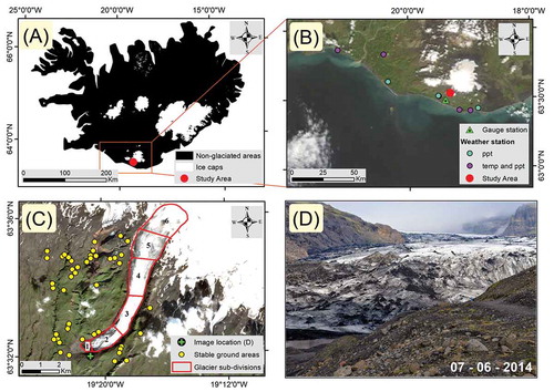
Sólheimajoküll is an 8-km long outlet glacier (Figure 1) with a mean thickness of 270 m that drains the Mýrdalsjökull ice cap in Southern Iceland (Staines et al. 2015). The glacier descends from 1350 to 100 m above sea level, where it terminates in a proglacial lake (Le Heron and Etienne 2005), which drains south through the Jökulsá á Sólheimasandi river to the Atlantic Ocean (Schomacker et al. 2012).

According to the Köppen climate classification (Kottek et al. 2006), Iceland has a polar tundra climate with a mean annual air temperature of 5.5°C and mean annual precipitation of 1610 mm (Source: Icelandic Meteorological Office station at Vatnsskarðshólar for the period 1949–2018). Over 80% of annual precipitation (rain and snow) falls between late September and May (Björnsson 1979). This is referred to as the accumulation period (Sigurđsson, Jónsson, and Jóhannesson 2007). During this time, as much as 10,000 mm/year of precipitation may fall across the central Mýrdalsjökull ice cap (Crochet et al. 2007).

Figure 1. (a) Location of ice caps in Iceland (white), non-glaciated areas (black) and study region (red). (b) Location of weather stations and gauge station in southern Iceland overlaid atop a true color composite image from Terra-MODIS (500 m spatial resolution) acquired on 18 August 2018. Blue circles are stations that record precipitation (ppt) only. Purple circles are stations that record ppt and temperature (temp). Stations are discussed in section 3: data is available at: https://en.vedur.is. (c) True color composite (band 4-3-2) Sentinel-2 satellite image acquired on 8 August 2018 overlaid with glacier sub-divisions (red lines) from the Randolph Glacier Inventory (RGI Consortium 2017) and 44 stable proglacial ground control points used for ice velocity uncertainty analysis (yellow). Green symbol specifies location of photo in (d), which is of the Solheimajokull glacier terminus taken on 7 June 2014 (photo by: Anikó Veres).

3. Data

To determine the advance and retreat of the glacier terminus, 21 multispectral satellite images (Landsat 1–8, Sentinel 1–2) were acquired from USGS Earth Explorer (https://earthexplorer.usgs.gov) and Copernicus scientific data hub (https://scihub.copernicus.eu) (Table S1). The requirements specified for image selection include: (1) < 60 m image spatial resolution, (2) cloud-free in the study area, and (3) acquisition date during or close to the ablation period. During years with more than one image that meets our selection criteria, we selected an end of melt season image. To classify glacial ice, false-color composite images were generated using the near-infrared band as the red channel, the green band as the green channel, and the blue band as the blue channel. Given that Landsat 1 MSS did not have a blue band, a composite image was established as the near-infrared band in the red channel, the red band in the green channel, and the green band in the blue channel.

We downloaded 113 Sentinel-1A Level 1 Interferometric WideSwath (IW) Ground Range Detected (GRD) images (Table S2), with ascending pass direction, at dual polarization, collected between Feb-2015 and Dec-2018 (~ two images per month). These images have 20 m spatial resolution, and only co-polarized bands of each SAR image were used (Schellenberger et al. 2016; Sánchez-Gámez and Navarro 2017).

Climatological data (temperature and precipitation) were obtained from the Icelandic Met Office (IMO) for eight weather stations located in Southern Iceland (https://en.vedur.is/climatology/data/#aa), which have been collecting weather data since 1949 (Table 1). The Icelandic weather observation network has changed over the last 30 years, with human observations being replaced by electronic sensors and data loggers. This improves data quality and traceability (Von Löwis and Þorvaldsson 2018), resulting in higher uncertainties for older measurements (Von Löwis and Þorvaldsson 2018; Jónsson and Garđarsson 2001). See Jónsson and Garđarsson (2001) for additional information about meteorological observations in Iceland.

Table 1. Weather station names, coordinates (decimal degrees), measurement period and variables measured (temp-temperature, ppt-precipitation).

Station name	Latitude (°)	Longitude (°)	Time period	Measured variables
Vatnsskarðshólar	63.424° N	−19.183°	1949–2018	temp,ppt
Skógar	63.527° N	−19.510°	1966–2011	ppt
Vík í Mýrdal	63.418° N	−19.008°	1961–2013	temp,ppt
Hella	63.834° N	−20.399°	1958–2004	temp,ppt
Kerlingardalur	63.433° N	−18.882°	2000–2017	ppt
Drangshlíðardalur	63.529° N	−19.520°	2012–2018	ppt
Eyrarbakki	63.866° N	−21.149°	1958–2016	temp,ppt
Bergþórshvoll	63.637° N	−20.332°	1962–1990	ppt

We also used hydrological records of water level (cm), temperature (°C) and conductivity (μS/cm) collected at gauge V263 on the Jökulsá á Sólheimasandi river located near the glacier terminus. These data are collected by the IMO, and are available at: http://vmkerfi.vedur.is/vatn/index.html. Note that the dynamic relationship between water level and discharge can be determined via mathematical relationships (Kumar 2011).

4. Methodology

4.1. Glacier terminus locations

The glacier terminus locations between 1973 and 2018 were manually mapped using optical satellite imagery (Table S1) and ESRI ArcMAP 10.4 GIS software. Advance and retreat cycles were measured relative to the terminus location, digitized in a Landsat-1 image acquired on 19 August 1973. Retreat was estimated relative to the central flow line of the glacier.

4.2. Glacier surface velocities

We used the Sentinel Application Platform (SNAP) software v6.0 developed by ESA (Serco Italia 2018) to measure glacier velocities. First, orbit data were appended to each image using the operator Orbit File. Second, the background energy generated by the sensor (i.e. thermal noise) was removed using look-up tables associated to each data product. Third, images were radiometrically calibrated. This procedure allows for comparison of SAR images acquired by the same sensor at different times. Thus, the images represent backscatter values (sigma nought, dB) in each pixel. We co-registered 112 image pairs in a consecutive manner over the study period. In each pair, the older image was assigned as the master and the newer image as the slave. For orthorectification, we used the 10 m resolution LMI Digital Elevation Model created by the National Land Survey of Iceland in 2016 (https://atlas.lmi.is/LmiData). Surface velocities were calculated using an offset-tracking algorithm, which estimates the movement of glacier surfaces between two consecutive pairs of co-registered SAR intensity images (master and slave), in both slant-range and azimuth direction (Strozzi et al. 2002). Horizontal ice displacements were estimated by determining the intensity cross-correlation peaks between patches of an image pair using a moving window (Wendleder, Friedl, and Mayer 2018). We used the offset-tracking algorithm implemented in the ESA SNAP software (Veci 2015; SNAP software, 2017). We thus assessed the velocity of the glacier in m/day within the time interval between image acquisitions. Given the local features of the study area, the offset-tracking algorithm was customized with registration window sizes of 60 × 60 pixels and a Ground Control Point (GCP) grid-spacing of 20 × 20 pixels (200 x 200 m), generating a total of 335 grid-points on the glacier surface. Velocity estimates of low confidence were discarded during the process using a cross-correlation coefficient threshold of 0.1. We set an approximation of the glacier’s maximum velocity of 5 m/day based on previous works (Eyþórsson et al. 1953; James, How, and Wynn 2016). The algorithm replaces velocity outliers by a new offset, which is computed as the local-weighted average within a window of four pixels, centered at the invalid GCP (Serco Italia 2018).

In addition, we removed erroneous offsets using a similar and combined routine described in Burgess et al. (2012) and Lüttig, Neckel, and Humbert (2017). The Randolph Glacier Inventory 6.0 (RGI Consortium 2017) was used to remove all off-ice vectors and to divide the glacier surface into sub-divisions according to the orientation of the glacier flow (Figure 1(c)). Thus, we highlight both the velocity gradient across the glacier, and the seasonal variations of the velocities. The algorithm then discards any displacement vector if its orientation differs by 24, 18 or 12 degrees from the average orientation computed over surrounding values (Burgess et al. 2012: Lippl, Vijay, and Braun 2018). In our case, these values were the data-points within a moving window of 25 pixels (5 x 5 pixels) with a pixel resolution of 200 × 200 m. In an effort to obtain the maximum number of velocity data-points and the lowest standard deviation, the orientation filter was run for four different angle values: 30, 24, 18, and 12 degrees. The last filter applied to delete the remaining low confidence estimates was based on Lüttig, Neckel, and Humbert (2017). We kept the data-points only when the absolute difference between the individual velocity point and the median velocity of the moving window was less than three times the standard deviation. The 30-degree threshold value reported the best trade-off in terms of variability and number of points filtered (Table S3), and Table S4 shows the percentage of the offsets removed by the applied filters (30-degree angle and velocity filter) per image-pair. We corrected topographical distortions and re-projected the SAR images using the Range–Doppler Terrain Correction operator (external digital elevation model: LMI 10 m, National Land Survey of Iceland and Map projection: WGS84utm27N).

We estimated the velocity uncertainty for each image pair following the same procedure as Wendleder, Friedl, and Mayer (2018), extracting displacement values at 44 distributed spots on non-glaciated surfaces (see Figure 1(c)). The suitable points were manually identified using an RGB image from Sentinel-2 (collected 18 August 2018). Mean uncertainties of the displacement fields per seasonal stack are provided in Table S5. Geographical data were represented using ArcMap ESRI and R software (R Core Team 2017).

River gauge data were compared with glacier velocities. We used five different time-response scenarios to choose the time-interval with the highest correlation. Scenario 0 relates glacier velocity estimates to water data during the same time period, i.e. between master and slave acquisition dates. The other four scenarios investigate time-delay intervals between velocity and hydrology data using the slave acquisition date (in each image pair) as reference. We therefore test 0–15 days after each slave acquisition date (scenario 15), 15–30 days (scenario 30), 30–45 days (scenario 45) and 45–60 days (scenario 60). This method allows us to calculate the correlation coefficient of each water parameter with respect to the velocity estimates and to evaluate which time scenario best represents the time lag between glacier dynamics and gauge data.

5. Results

5.1. Glacier terminus advance and retreat

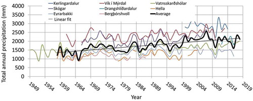
We analyzed temperature and precipitation records in southern Iceland. Temperature records indicate a cooling period from the early 1950s until the late 1970s, followed by a warming trend (Figure 2). Precipitation records report two different trends. From the early 50s until the mid-60s, precipitation rates remained constant between the range 1000–1500 mm/year (Figure 3). However, the average precipitation started to increase after the mid-60s to between 1500 and 2500 mm/year.

Figure 2. Mean annual temperature at four weather stations in southern Iceland (blue, green, red and purple lines). The annual average of the four stations is also plotted (black line). Linear fit for the annual average is given for the periods 1958–1979 and 1980–2019 (gray line).

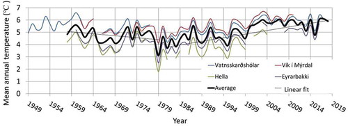
Figure 3. Total annual precipitation (mm we) measured at eight weather stations in southern Iceland. The average of the cumulative annual values at each station is plotted (black line). The linear fit of the average is also shown (gray line).

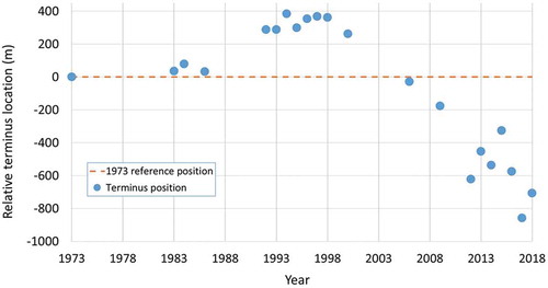
The advance and retreat of the glacier terminus location over 45 years is shown in Figure 4. The earliest satellite image dates from August 1973, since when the glacier terminus has retreated approximately 685 m. There are two dominant trends: the glacier advanced from 1973 to 1998, and has since continued to retreat. Over the last 18 years, the Solheimajoküll glacier has retreated 970 m. In the same period, the mean annual temperature has ranged from 4.7 to 6.1°C. These persistent high temperatures are unprecedented across the meteorological station (Figure 2).

Figure 4. Solheimajoküll glacier terminus advance and retreat (m) relative to the 1973 position (blue dots). Positive values represent glacier advance and negative values glacier retreat. Table S1 lists collection date and satellite data used for terminus mapping.

5.2. Glacier surface velocities

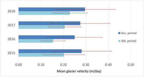
The ice velocity of the Solheimajoküll glacier during ablation (Jun – Sept) and accumulation (Oct – May) periods between 2015 and 2018 is plotted in Figure 5. The mean velocity was 0.28 ± 0.13 m/day during the accumulation period, dropping to 0.20 ± 0.07 m/day during the ablation period. Surface velocity during the ablation period has increased since 2016. In addition, uncertainty is higher during accumulation periods when rates remain relatively constant, ranging from 0.26 ± 0.10 to 0.30 ± 0.15 m/day.

Figure 5. Mean glacier surface velocity (m/day) for accumulation (Acc., dark-blue) and ablation (Abl., light-blue) periods from 2015 to 2018. Mean uncertainty is plotted in red.

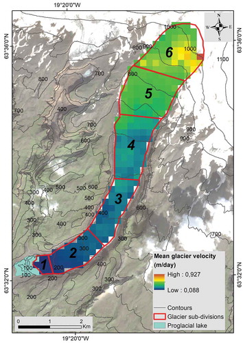
Surface velocity tends to be fastest at higher ice-surface elevations (Table S6 and Figure 6). For example, sub-division 1 has a mean velocity of 0.10 m/day (Std. = 0.05), while sub-divisions 2, 3, 4, 5 and 6 have increasingly faster average velocities of 0.14 m/day (Std. = 0.06), 0.18 m/day (Std. = 0.09), 0.23 m/day (Std. = 0.12), 0.38 m/day (Std. = 0.16), and 0.49 m/day (Std. = 0.22).

Figure 6. Mean ice velocity for the Solheimajoküll glacier tongue, Iceland mapped using Sentinel-1 synthetic aperture radar (SAR) images collected between February 2015 and March 2018. Surface topography contours are represented by gray lines, the proglacial lake location is shown (blue) and glacier sub-divisions are mapped atop the average velocity layer. Background image corresponds to Sentinel-2 acquired on 8 August 2018.

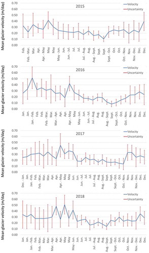
Figure 7 shows the mean ice velocity (m/day) and mean uncertainty (m/day) for Solheimajoküll glacier estimated at each image pair between 2015 and 2018. The highest velocities with the lowest uncertainties were recorded from mid-April to June.

Figure 7. Mean glacier velocities of Solheimajoküll (blue) estimated at each image pair from 2015 to 2018 (m/day), and mean uncertainties (red) over the same period (m/day).

Ice velocities were compared to hydrological data following different time-response scenarios. Table 2 shows the average values of air temperature and hydrological data for the accumulation and ablation periods. The Pearson correlation coefficient can be used to evaluate the statistical relationship between two continuous variables, indicating the magnitude and direction of the association (Schober, Boer, and Schwarte 2018). It ranges from −1 (negative correlation) to 1 (positive correlation), with values close to zero indicating no correlation. Figure 8 shows the correlation coefficient calculated between glacier velocities and water parameters for each time-lag tested.

Figure 8. Evaluation of time lag potentials, tested as 0, 15, 30, 45, and 60 day lags. The Pearson correlation coefficient is calculated between Solheimajoküll glacier ice velocity and hydrological parameters, including: mean water level (MeanWL, blue), mean water temperature (MeanWT, yellow), and mean water conductivity (MeanWC, pink). Reference lines (dashed green) indicate moderate positive and negative correlation values among variables (Corder and Foreman 2009).

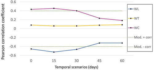
Table 2. Average values of water level (WL), water temperature (WT), water conductivity (WC) and air temperature (AT) for the accumulation (Acc.) and ablation (Abl.) periods.

Period	Mean WL (cm)	Mean WT (°C)	Mean WC (μS/cm)	Mean AT (°C)
Acc.	390.55	2.4	115.14	3.6
Abl.	414.00	2.9	75.94	9.9

Moderate correlations were found for water conductivity and water level in scenarios 0, 15, and 30, whereas after 30 days from the slave acquisition date, there is no significant correlation with glacier velocities. The mean water temperature indicated no correlation across all the time scenarios tested. Thus, the time-lag between glacier velocities and gauge data would be better explained using the temporal coverage of scenarios 0, 15, and 30 altogether using all the available data. To further investigate the seasonality of the time-lag, we split the dataset by months of the year. Table 3 shows the correlation coefficients between glacier velocities and water data across scenarios 0, 15, 30, 45, and 60, discarding winter months from the analysis given their high uncertainty.

Table 3. Pearson correlation coefficients for the relation of glacier velocities and gauge data (MeanWL: mean water level, MeanWT: mean water temperature and MeanWC: mean water conductivity) by months across scenarios 0, 15, 30, 45, and 60. Note that winter months (Nov., Dec., Jan., Feb. and Mar.) have not been included in the table due to the high uncertainties associated to those glacier velocities.

			Mean WL
Month	Scenario 0	Scenario 15	Scenario 30	Scenario 45	Scenario 60
Apr.	0.77	0.41	0.39	0.41	0.37
May.	−0.21	−0.17	−0.27	−0.28	−0.25
Jun.	0.09	0.19	0.12	0.25	0.29
Jul.	0.45	0.36	0.36	0.35	0.32
Aug.	0.74	0.59	0.45	0.37	0.35
Sep.	0.23	−0.25	−0.55	−0.47	−0.35
Oct.	−0.78	−0.81	−0.77	−0.76	−0.75
			Mean WT
Month	Scenario 0	Scenario 15	Scenario 30	Scenario 45	Scenario 60
Apr.	0.60	0.23	0.22	0.23	0.25
May.	−0.16	−0.08	−0.05	−0.04	−0.04
Jun.	−0.21	−0.28	−0.29	−0.29	−0.29
Jul.	0.76	0.80	0.80	0.80	0.80
Aug.	0.50	0.37	0.36	0.37	0.34
Sep.	0.06	0.23	0.21	0.17	0.15
Oct.	−0.25	−0.38	−0.47	−0.53	−0.57
			Mean WC
Month	Scenario 0	Scenario 15	Scenario 30	Scenario 45	Scenario 60
Apr.	−0.54	−0.36	−0.38	−0.41	−0.39
May.	−0.04	−0.16	−0.18	−0.22	−0.18
Jun.	0.10	0.38	0.52	0.60	0.58
Jul.	−0.36	−0.30	−0.31	−0.41	−0.48
Aug.	0.17	0.10	−0.08	−0.04	−0.02
Sep.	0.25	0.03	0.15	0.29	0.33
Oct.	0.60	0.63	0.67	0.81	0.87

Water temperature was positively correlated with ice velocity in April, July and August, and negatively correlated in October. There was no correlation in May, June and September. Scenarios 0 and 15 presented the highest scores across the correlated months, with the exception of October (scenario 60). Figures S2 and S3 show a positive correlation between air and water temperature, although the latter usually reaches its maximum in May or June (1–2 months before air temperature does), just when the water level begins to increase as the glacier drainage becomes more efficient.

The mean water level showed a positive correlation with ice velocity in April, July and August (scenario 0), and a negative correlation in September and October (scenarios 15 and 30). Between August and September, there was a transitional period after which the glacier decelerates as the water level increases, indicating the beginning of the stagnant phase of the glacier. It is worth noting a break in the trend of the temporal analysis (May and June), which can be explained by the temporal decorrelation of glacier dynamics across years (e.g. meltwater onset, glacier drainage evolution). To better visualize these temporal decorrelations, we plotted all the velocity estimates with respect to their associated water parameters (using scenario 0, 15 and 30 altogether) and aggregated them by months of the year (Fig. S5-7).

Glacier velocities had a moderate negative correlation with water conductivity for April (scenario 0) and July (scenario 60), while strong positive correlations were found in June (scenario 45) and October (scenario 60). Water level and water conductivity displayed a typically negative correlation (Fig. S1, S4). However, as the river partly drains meltwater generated by geothermal activity under Mýrdalsjökull ice cap, both water variables might be positively correlated for short periods of the year.

6. Discussion

6.1. Glacier terminus analysis

There have been two regional temperature trends that correlate with glacier dynamics. There was a cooling period from 1949 to 1979 (Figure 2), which coincided with an advance of Icelandic glaciers until the 1990s (Sigurđsson, Jónsson, and Jóhannesson 2007), followed by a warming period which continues today. Satellite imagery shows similar patterns in the extent of the Solheimajoküll glacier (Figure 4), which has been retreating since the early 21^st century. There is a time lag between the end of the cooling period (by 1979) and the retreat of the glacier termini (after 1998). This is explained by Crochet et al. (2007), who indicate that glacier termini do not react immediately to mass-balance changes, but with a delay of a few years. From 1996 to 2010, glacier volume decreased by 0.106 km³ (Staines et al. 2015), confirming the negative mass balance of the Solheimajoküll glacier. The observed glacier extent (Figure 4) is then affected by climate changes in the study area (Mackintosh, Dugmore, and Hubbard 2002; Crochet et al. 2007; Staines et al. 2015). Between 2000 and 2018, Solheimajoküll retreated at ~ 53 m/year, which is comparable to many other glacier change rates in Iceland (Chandler, Evans, and Roberts 2016).

6.2. Glacier surface velocities

Ice-surface velocity (Jóhannesson et al. 2004) and summer temperatures (Huss et al. 2008) are indicators of glacier retreat. Seasonal analysis of Solheimajoküll velocities suggests a slight acceleration during the ablation season since 2016, whereas velocities during the accumulation season remained constant. The spatial analysis of the 4-year period indicates a velocity increase relative to the terminus distance (Table S6), ranging from 0.10 m/day (Std. = 0.05) to 0.49 m/day (Std. = 0.22) on average. Maximum velocities were detected at high elevations where the ice-surface slope is steepest (Figure 6), consistent with observations of other glaciers (Sam et al. 2018; Fan et al. 2019). The 4-year surface velocity average was 0.26 ± 0.11 m/day (Table S6), which is similar to results obtained by Eyþórsson et al. (1953) and James, How, and Wynn (2016) at Solheimajoküll, reporting speeds of 0.06 to 1.24 m/day. The latter study used oblique time-lapse imagery at Solheimajoküll to retrieve a mean ice velocity of 0.17 ± 0.02 m/day in a time period of 73 days (May to July). The highest velocities with the lowest uncertainties were recorded from mid-April to June (Figure 7). During the accumulation season, glacier velocities were constant (Figure 5), consistent with a closure of the subglacial drainage system.

Glacier velocity can be measured by manual survey (e.g. in-situ stakes), ground-based cameras or remote-sensing techniques (Watson and Quincey 2015). Manual surveys can achieve centimeter accuracy, but have notable limitations including cost, glacier access, hazardous debris coverage glaciers, added to which they are time-consuming to conduct (Watson and Quincey 2015). Ground-based camera methods pose other challenges such as limited solar illumination during winter, snow cover, weather variability or ground instability (James, How, and Wynn 2016). Similarly, cloud cover can be a handicap in optical satellite remote sensing. Hence, SAR imagery from Sentinel-1 coupled with the proposed offset-tracking technique is a convenient and cost-effective tool for monitoring glacier velocities. The main uncertainties derived from the offset-tracking method include ionospheric disturbances, geocoding, co-registration errors, and/or environmental factors (Rankl, Kienholz, and Braun 2014; Nagler et al. 2015). It is therefore important to assess the velocity uncertainty of each image pair estimating displacement values over non-moving terrain; avoiding snow, ice, river beds, terraces or vegetation (Rankl, Kienholz, and Braun 2014).

In southern Iceland, the ground is snow covered most of the year, while during summer, vegetation covers stable rock outcrops. Given this, we used a high-resolution DEM (10 m) with co-registration to mitigate the effect of snow and vegetation (Barazzetti, Scaioni, and Gianinetto 2014). Nevertheless, some of the velocities measured (e.g. during snowy months) should be interpreted with caution given uncertainty in the co-registration of image pairs.

We used five time-response scenarios to identify time-lags between Solheimajoküll surface velocity and downstream water quantity and quality parameters (Fig. 8). Overall, a 30-day time-window exhibited the highest correlation between velocity and water parameters. To address glacier evolution across the year, we investigated the direction and magnitude of the correlations between glacier velocities and gauge data, and tested the proposed time-lag scenarios by months. Thus, we infer the efficiency of the subglacial system as a reduction in ice velocity as the melt season progresses. Table 3 suggests that time lags between ice velocities and gauge data are variable throughout the year, and may also vary across different years (Fig. S5-7).

For the water level parameter, we obtained positive correlations between glacier velocities and gauge data from April, July and August, and negative correlations during September and October (Table 3), indicating that the drainage system becomes more efficient as the melt season progresses and ice velocities decelerate. In April, July and August, the correlations decreased from scenario 0 to scenario 60, indicating a rapid time response between glacier velocities and water level. Glacier velocities may be influenced by a seasonal increase in air temperature (Figure S3), which likely enhances meltwater drainage from the surface, increasing basal motion. Many studies have demonstrated that meltwater runoff is highly sensitive to air temperature (Lang 1973; Sun et al. 2015; Li et al. 2016). The lag time between both variables varies across months in the melting season and is not uniform for different glaciers (Xie et al. 2006; Li et al. 2016). However, meltwater production can be modulated by the glacier hydrological, non-channelized ice-surface conditions (weathering crust, firn, albedo, etc.) (Lampkin and VanderBerg 2014; Dragosics et al. 2016; Lenaerts et al. 2017; Nienow et al. 2017). Between August and September, velocity estimates indicate a deceleration, likely attributed to the drainage system becoming more efficient, which results in decreases in basal water pressure. Table 3 indicates time lags between 15 and 30 days for September and October. These results concur with previous studies such as Vincent and Moreau (2016) who relate ice-flow velocities to subglacial water runoff changes at a seasonal scale. In the latter study, they observed glacier velocity increase during the beginning of the ablation period, which then decreased as the subglacial drainage system became efficient at the end of the melt season. Thus, Solheimajoküll velocities observed from May to August would be conditioned by an increase in the basal water pressure at the ice–bed interface, which reduces basal friction (Boulton et al. 2007, Paterson 2016). September and October ice velocities tend to decrease as the subglacial drainage system becomes more efficient. This implies that the amount of basal water pressure decrease and basal friction increases (Boulton et al. 2007).

Water level and conductivity generally negatively correlated with ice velocity (Fig. S1, S4), suggesting that geothermal water contribution to river discharge is minimal. Significant geothermal or volcanic events often positively correlate with discharge and conductivity in glacial rivers (Lawler, Björnsson, and Dolan 1996; Kristmannsdóttir et al. 1999). The dynamic relationship between water level and discharge can be determined via mathematical relationships (Kumar 2011). Unlike water level, the highest positive correlations between ice velocity and water conductivity were obtained under scenario 45 (June) and 60 (July and October) indicating a longer time response. April and July evidence negative correlations as the water level increases. It is worth noting the positive correlation found in June, which contrasts with the negative correlations of April and July. Han et al. (2015) observed a similar relationship between conductivity and discharge in the early ablation season. The positive correlation found in June suggests a seasonal release of geothermal water generated during the accumulation season. Despite the negative conductivity trend during April, May and June (Fig. S4), some disruptions in the mean values (with temporary increases) were found in the time series: 4^th-31 July 2015, 18^th-15 July 2016 and 20^th-17 July 2018. The fraction of geothermal water is much smaller than meltwater runoff during the summer melt season (Han et al. 2015). Winter gauge data are more sensitive to variations in water conductivity; hence, weak anomalies caused by geothermal or volcanic activity are easier to identify. A sudden rise in water conductivity might be related to the leakage of geothermal fluids into the subglacial drainage network (Lawler, Björnsson, and Dolan 1996; Kristmannsdóttir et al. 1999), although site-specific monitoring of meltwater conductivity is required to determine a precursor threshold for volcanic events and jökulhlaups (Tuladhar 2017). Lawler, Björnsson, and Dolan (1996) observed hydrochemical perturbations and a sudden significant increase in flow of the Jökulsá á Sólheimasandi river with a time lag of 11 days after detecting subglacial geothermal fluid injection under Myrdalsjökull, the parent ice cap of Solheimajoküll. Sudden changes in subglacial water flow also affect glacier velocities after geothermal and/or volcanic episodes. For instance, Magnússon et al. (2010) detected a glacier velocity decrease of more than 50% after a jökulhlaup at a glacier outlet in the Vatnajökull ice cap. In Iceland, this type of glacial outburst flood may originate from meltwater generated by geothermal heat flux, atmospheric processes or volcanic eruptions (Björnsson 2009).

In summary, we propose a methodology to monitor surface glacier velocities using the open-access SNAP software. The velocity-time series at the Solheimajoküll glacier suggest acceleration during the summer melt season since 2016, whereas glacier velocities during accumulation months were constant. The hydrological time response to glacier accelerations was found to be between one and thirty days after the velocity estimates. Additionally, the analysis of glacier terminus locations indicates a retreat rate of −53 m/year since 2000, which is comparable to many other glacier change rates in Iceland.

7. Conclusions

In this study, we investigate linkages between the climate of southern Iceland and Solheimajoküll glacier dynamics. We show that Sentinel-1 is a cost-effective technology for monitoring glacier dynamics, regardless of weather or solar conditions.

Variations in mean annual temperatures have resulted in advances and retreats of the Solheimajoküll terminus over the last 50 years. A time lag of approximately 19 years is identified between the end of the cooling period (1979) and the onset of terminus retreat (1998). Glacier retreat at Solheimajoküll coincides with the gradual increase in mean annual temperatures in southern Iceland over the last 40 years or so, and indicates a change in regional climate.

Our velocity estimates suggest an acceleration during the ablation period since 2016, whereas velocities during accumulation periods remain constant. The highest velocities were observed at high elevations, where the slope is the steepest. We tested several scenarios to assess the hydrological time response after glacier velocity, and the highest correlations were found between one and thirty days. Monthly correlations suggest inter-annual and intra-annual variability in the glacier dynamics. Glacier velocities positively correlated with water level from April to August, but negatively correlated with water conductivity. We also noted a temporary disruption in correlations between water conductivity and June glacier velocities. The water level and conductivity time series may suggest a seasonal release of geothermal water generated during the accumulation season.

Author contributions

Conceptualization, D.G. and J.C.; Methodology, D.G. and P.S.; Formal Analysis, D.G., P.S. and M.U.; Validation, D.G., P.S. and M.U.; Data Curation, D.G., J.S. and J.C., Writing—Original Draft Preparation, D.G., Writing—Review & Editing, D.G., P.S., J.C, J.S. and M.U.; Supervision, J.S. and J.C.; Project Administration, J.S.

Acknowledgements

The authors wish to acknowledge the support provided by the Copernicus Research and User Support Service (RUS), and would like to thank the European Space Agency (ESA) and the National Aeronautics and Space Administration (NASA) for offering free access to satellite imagery. In addition, we wish to express our gratitude to the Icelandic Met Office (Veðurstofa Íslands) for providing free-access data about the past climate of Iceland, as well as hydrological data from river gauge stations. We also thank the anonymous reviewers for their constructive comments, which helped us enormously in improving the manuscript and rendering its final form.

Disclosure statement

All authors declare that they have no conflict of interest.

Supplementary material

Supplemental data for this article can be accessed here.

Additional information

Funding

This work did not receive any funding.

References

- Anderson, L. S., Á. Geirsdóttir, G. E. Flowers, A. D. Wickert, G. Aðalgeirsdóttir, and T. Thorsteinsson. 2019. “Controls on the Lifespans of Icelandic Ice Caps.” Earth and Planetary Science Letters 527: 115780. doi:10.1016/j.epsl.2019.115780.
- Andreason, J. O. 1985. “Seasonal Surface‐velocity Variations on a Sub‐polar Glacier in West Greenland.” Journal of Glaciology 31 (109): 319–323. doi:10.1017/S0022143000006651.
- Barazzetti, L., M. Scaioni, and M. Gianinetto. 2014. “Automatic Co-registration of Satellite Time Series via Least Squares Adjustment.” European Journal of Remote Sensing 47 (1): 55–74. doi:10.5721/EuJRS20144705.
- Bartholomaus, T. C., R. S. Anderson, and S. P. Anderson. 2008. “Response of Glacier Basal Motion to Transient Water Storage.” Nature Geoscience 1 (1): 33. doi:10.1038/ngeo.2007.52.
- Bermudez, J. D., P. N. Happ, D. A. B. Oliveira, and R. Q. Feitosa. 2018. “SAR to Optical Image Synthesis for Cloud Removal with Generative Adversarial Networks.” ISPRS Annals of Photogrammetry, Remote Sensing & Spatial Information Sciences 4: 1.
- Björnsson, H. 1979. “Glaciers in Iceland.” Jokull 29: 74–80.
- Björnsson, H. 2009. Jokulhlaups in Iceland: Sources, Release and Drainage, 50–64. Cambridge: Megaflooding on Earth and Mars. Cambridge University Press.
- Björnsson, H. 2017. “Glaciers of the Central Highlands.” In The Glaciers of Iceland. Atlantis Advances in Quaternary Science, Vol. 2. Paris: Atlantis Press. doi:10.2991/978-94-6239-207-6_6.
- Björnsson, H., and F. Pálsson. 2008. “Icelandic Glaciers.” Jökull 58: 365–386.
- Björnsson, H., F. Pálsson, and M. T. Guðmundsson. 2000. “Surface and Bedrock Topography of the Mýrdalsjökull Ice Cap.” Jökull 49: 29–46.
- Björnsson, H., F. Pálsson, S. Gudmundsson, E. Magnússon, G. Adalgeirsdóttir, T. Jóhan-nesson, E. Berthier, O. Sigurdsson, and T. Thorsteinsson. 2013. “Contribution of Icelandic Ice Caps to Sea Level Rise: Trends and Variability since the Little Ice Age.” Geophysical Research Letters 40 (8): 1546–1550. doi:10.1002/grl.50278.
- Bolton, L. J. 2013. “Temperature Variations of Runoff from Highly-glacierised Alpine Basins.” Doctoral dissertation, University of Salford). Accessed March 15 2020. http://usir.salford.ac.uk/id/eprint/30248
- Boulton, G. S., R. Lunn, P. Vidstrand, and S. Zatsepin. 2007. “Subglacial Drainage by Groundwater-channel Coupling, and the Origin of Esker Systems: Part 1—glaciological Observations.” Quaternary Science Reviews 26 (7–8): 1067–1090. doi:10.1016/j.quascirev.2007.01.007.
- Braithwaite, R. J., and O. B. Olesen. 1989. “Calculation of Glacier Ablation from Air Temperature, West Greenland.” Glacier Fluctuations and Climatic Change, Springer, Dordrecht 219–233. doi:10.1007/978-94-015-7823-3_15.
- Brown, G. H. 2002. “Glacier Meltwater Hydrochemistry.” Applied Geochemistry 17 (7): 855–883. doi:10.1016/S0883-2927(01)00123-8.
- Burgess, E. W., R. R. Forster, C. F. Larsen, and M. Braun. 2012. “Surge Dynamics on Bering Glacier, Alaska, in 2008–2011.” The Cryosphere 6 (6): 1251–1262. doi:10.5194/tc-6-1251-2012.
- Chandler, B. M., D. J. Evans, and D. H. Roberts. 2016. “Recent Retreat at a Temperate Icelandic Glacier in the Context of the Last~ 80 Years of Climate Change in the North Atlantic Region.” Arktos 2 (1): 24. doi:10.1007/s41063-016-0024-1.
- Chu, V. W. 2014. “Greenland Ice Sheet Hydrology.” Progress in Physical Geography: Earth and Environment 38 (1): 19–54. doi:10.1177/0309133313507075.
- Consortium, R. G. I. 2017. Randolph Glacier Inventory – A Dataset of Global Glacier Outlines: Version 6.0: Technical Report, Global Land Ice Measurements from Space. Colorado, USA: Digital Media. doi:10.7265/N5-RGI-60.
- Corder, G. W., and D. I. Foreman. 2009. “Nonparametric Statistics for Non‐statisticians.” John Wiley & Sons, Inc. doi:10.1002/9781118165881.
- Crochet, P., T. Jóhannesson, T. Jónsson, O. Sigurðsson, H. Björnsson, F. Pálsson, and I. Barstad. 2007. “Estimating the Spatial Distribution of Precipitation in Iceland Using a Linear Model of Orographic Precipitation.” Journal of Hydrometeorology 8 (6): 1285–1306. doi:10.1175/2007JHM795.1.
- Das, S. B., I. Joughin, M. D. Behn, I. M. Howat, M. A. King, D. Lizarralde, and M. P. Bhatia. 2008. “Fracture Propagation to the Base of the Greenland Ice Sheet during Supraglacial Lake Drainage.” Science 320 (5877): 778. doi:10.1126/science.1153360.
- Davison, B. J., A. J. Sole, S. J. Livingstone, T. R. Cowton, and P. W. Nienow. 2019. “The Influence of Hydrology on the Dynamics of Land-terminating Sectors of the Greenland Ice Sheet.” Frontiers in Earth Science 7: 10. doi:10.3389/feart.2019.00010.
- De Angelis, H., and P. Skvarca. 2003. “Glacier Surge after Ice Shelf Collapse.” Science 299 (5612): 1560–1562. doi:10.1126/science.1077987.
- Dowdeswell, J. A., J. O. Hagen, H. Björnsson, A. F. Glazovsky, W. D. Harrison, P. Holmlund, and R. H. Thomas. 1997. “The Mass Balance of circum-Arctic Glaciers and Recent Climate Change.” Quaternary Research 48 (1): 1–14. doi:10.1006/qres.1997.1900.
- Dragosics, M., O. Meinander, T. Jónsdóttír, T. Dürig, G. De Leeuw, F. Pálsson, and T. Thorsteinsson. 2016. “Insulation Effects of Icelandic Dust and Volcanic Ash on Snow and Ice.” Arabian Journal of Geosciences 9 (2): 126. doi:10.1007/s12517-015-2224-6.
- Dussaillant, A., G. Benito, W. Buytaert, P. Carling, C. Meier, and F. Espinoza. 2010. “Repeated Glacial-lake Outburst Floods in Patagonia: An Increasing Hazard?” Natural Hazards 54 (2): 469–481. doi:10.1007/s11069-009-9479-8.
- Eberhardt, I. D. R., B. Schultz, R. Rizzi, I. D. A. Sanches, A. R. Formaggio, C. Atzberger, and L. A. José Barreto. 2016. “Cloud Cover Assessment for Operational Crop Monitoring Systems in Tropical Areas.” Remote Sensing 8 (3): 219. doi:10.3390/rs8030219.
- Einarsson, B. 2012. “Available Discharge Time-series from Glacier-covered Catchments in Iceland.” Veðurstofa Íslands Technical Report. Accessed April 28 2019. http://ncoe-svali.org/xpdf/be_2012_01.pdf
- Erten, E., A. Reigber, O. Hellwich, and P. Prats. 2009. “Glacier Velocity Monitoring by Maximum Likelihood Texture Tracking.” IEEE Transactions on Geoscience and Remote Sensing 47 (2): 394–405. doi:10.1109/TGRS.2008.2009932.
- ESRI. 2016. ArcMap 10.4. Redlands, CA: Environmental Systems Research Institute.
- Eyþórsson, J., H. Lister, R. Jarvis, M. McDonald, I. W. Paterson, R. Walker, and N. Í Reykjavík. 1953. “Sólheimajökull: Report of the Durham University Iceland Expedition 1948.” Acta Naturalia Islandica 1 (8). Accessed March 25 2019. http://hdl.handle.net/10802/10050
- Fan, J., Q. Wang, G. Liu, L. Zhang, Z. Guo, L. Tong, Z. Perski. 2019. “Monitoring and Analyzing Mountain Glacier Surface Movement Using SAR Data and A Terrestrial Laser Scanner: A Case Study of the Himalayas North Slope Glacier Area.” Remote Sensing 11 (6): 625. doi:10.3390/rs11060625.
- Fountain, A. G., and J. S. Walder. 1998. “Water Flow through Temperate Glaciers.” Reviews of Geophysics 36 (3): 299–328. doi:10.1029/97RG03579.
- Grove, J. M. 2013. Little Ice Ages. Routledge. 1 (2). ISBN 9780203770245 doi:10.4324/9780203770269.
- Guan, M., N. G. Wright, P. A. Sleigh, and J. L. Carrivick. 2015. “Assessment of hydro-morphodynamic modelling and geomorphological impacts of a sediment-charged jökulhlaup, at Sólheimajökull, Iceland”. Journal of Hydrology 530: 336–349. https://doi.org/10.1016/j.jhydrol.2015.09.062
- Gudmundsson, G. H. 2003. “Transmission of Basal Variability to a Glacier Surface.” Journal of Geophysical Research: Solid Earth 108 (B5): 2253. doi:10.1029/2002JB002107.
- Gunnlaugsson, Á. Þ., E. Magnússon, P. Pálsson, J. M. C. Belart, and Þ. Árnadóttir. 2016. “Surface Elevation Changes of Mýrdalsjökull Ice-cap: 1960-2010.” Accessed March 25 2019. http://www.norvol.hi.is/~thora/Mass_loss_of_Myrdalsjokull_ice_cap_RH11_2016.pdf
- Han, T., X. Li, M. Gao, M. Sillanpää, H. Pu, and C. Lu. 2015. “Electrical Conductivity during the Ablation Process of the Glacier No. 1 At the Headwaters of the Urumqi River in the Tianshan Mountains.” Arctic, Antarctic, and Alpine Research 47 (2): 327–334. doi:10.1657/AAAR00C-13-138.
- Hodson, A., J. Kohler, M. Brinkhaus, and P. Wynn. 2005. “Multi-year Water and Surface Energy Budget of a High-latitude Polythermal Glacier: Evidence for Overwinter Water Storage in a Dynamic Subglacial Reservoir.” Annals of Glaciology 42: 42–46. doi:10.3189/172756405781812844.
- Hoffman, M. J., L. C. Andrews, S. F. Price, G. A. Catania, T. A. Neumann, M. P. Lüthi, and B. Morriss. 2016. “Greenland Subglacial Drainage Evolution Regulated by Weakly Connected Regions of the Bed.” Nature Communications 7 (1): 1–12. doi:10.1038/ncomms13903.
- Holden, J., Ed. 2005. An Introduction to Physical Geography and the Environment. Essex: Pearson Education.
- Houghton, J. 2004. Mass Balance of the Cryosphere: Observations and Modelling of Contemporary and Future Changes. Cambridge University Press. doi:10.1017/CBO9780511535659.
- Huss, M., A. Bauder, M. Funk, and R. Hock. 2008. “Determination of the Seasonal Mass Balance of Four Alpine Glaciers since 1865.” Journal of Geophysical Research: Earth Surface 113 (F1): F1. doi:10.1029/2007JF000803.
- Irvine‐Fynn, T. D. L., A. J. Hodson, B. J. Moorman, G. Vatne, and A. L. Hubbard. 2011. “Polythermal Glacier Hydrology.” A Review, Rev. Geophys 49: RG4002. doi:10.1029/2010RG000350.
- Irvin-Fynn, T. D. L., B. J. Moorman, I. C. Willis, I. C. Sjogren, A. J. Hodson, P. N. Mumford, and J. L. M. Williams. 2005. “Geocryological Processes Linked to High Arctic Proglacial Stream Suspended Sediment Dynamics: Examples from Bylot Island, Nunavut, and Spitsbergen, Svalbard.” Hydrological Processes 19 (1): 115–135. doi:10.1002/hyp.5759.
- Jaenicke, J., C. Mayer, K. Scharrer, U. Münzer, and Á. Gudmundsson. 2006. “The Use of Remote-sensing Data for Mass-balance Studies at Mýrdalsjökull Ice Cap, Iceland.” Journal of Glaciology 52 (179): 565–573. doi:10.3189/172756506781828340.
- James, M. R., P. How, and P. M. Wynn. 2016. “Pointcatcher Software: Analysis of Glacial Time-lapse Photography and Integration with Multitemporal Digital Elevation Models.” Journal of Glaciology 62 (231): 159–169. doi:10.1017/jog.2016.27.
- Jóhannesson, T., G. Adalgeirsdóttir, H. Björnsson, F. Pálsson, and O. Sigurdsson 2004. “Response of Glaciers and Glacier Runoff in Iceland to Climate Change.” In Nordic Hydrological Conference 2004 (NHC-2004), 651–660. Accessed March 25 2019. https://www.researchgate.net/profile/Gudfinna_Adalgeirsdottir/publication/242398661_RESPONSE_OF_GLACIERS_AND_GLACIER_RUNOFF_IN_ICELAND_TO_CLIMATE_CHANGE/links/0046353c55d5c63c7c000000/RESPONSE-OF-GLACIERS-AND-GLACIER-RUNOFF-IN-ICELAND-TO-CLIMATE-CHANGE.pdf
- Jónsson, T., and H. Garđarsson. 2001. “Early Instrumental Meteorological Observations in Iceland.” Climatic Change 48 (1): 169–187. doi:10.1023/A:1005617512142.
- Kottek, M., J. Grieser, C. Beck, B. Rudolf, and F. Rubel. 2006. “World Map of the Köppen-Geiger Climate Classification Updated.” Meteorologische Zeitschrift 15 (3): 259–263. doi:10.1127/0941-2948/2006/0130.
- Kraaijenbrink, P., S. W. Meijer, J. M. Shea, F. Pellicciotti, S. M. De Jong, and W. W. Immerzeel. 2016. “Seasonal Surface Velocities of a Himalayan Glacier Derived by Automated Correlation of Unmanned Aerial Vehicle Imagery.” Annals of Glaciology 57 (71): 103–113. doi:10.3189/2016AoG71A072.
- Kristmannsdóttir, H., A. Björnsson, S. Pálsson, and Á. E. Sveinbjörnsdóttir. 1999. “The Impact of the 1996 Subglacial Volcanic Eruption in Vatnajökull on the River Jökulsá Á Fjöllum, North Iceland.” Journal of Volcanology and Geothermal Research 92 (3–4): 359–372. doi:10.1016/S0377-0273(99)00056-6.
- Kumar, A. 2011. “Stage-Discharge Relationship.” In Encyclopedia of Snow, Ice and Glaciers. Encyclopedia of Earth Sciences Series, edited by V. P. Singh, P. Singh, and U. K. Haritashya. Dordrecht: Springer. doi:10.1007/978-90-481-2642-2.
- Lampkin, D. J., and J. VanderBerg. 2014. “Supraglacial Melt Channel Networks in the Jakobshavn Isbræ Region during the 2007 Melt Season.” Hydrological Processes 28 (25): 6038–6053. doi:10.1002/hyp.10085.
- Lang, H. 1973. “Variations in the Relation between Glacier Discharge and Meteorological Elements.” versuchsanstalt fuer wasserbau, hydrologie und glaziologie, eth zuerich, 85–94. Accessed August 13 2020. http://hydrologie.org/redbooks/a095/iahs_095_0085.pdf
- Lawler, D. M., H. Björnsson, and M. Dolan. 1996. “Impact of Subglacial Geothermal Activity on Meltwater Quality in the Jökulsá Á Sólheimasandi System, Southern Iceland.” Hydrological Processes 10 (4): 557–577. doi:10.1002/(SICI)1099-1085(199604)10:4<557:aid-hyp392>3.0.CO;2-O.
- Le Heron, D. P., and J. L. Etienne. 2005. “A Complex Subglacial Clastic Dyke Swarm, Sólheimajökull, Southern Iceland.” Sedimentary Geology 181 (1–2): 25–37. doi:10.1016/j.sedgeo.2005.06.012.
- Lemke, P., J. Ren, R. B. Alley, I. Allison, J. Carrasco, G. Flato, and T. Zhang. 2007. Changes in Glaciers and Ice Caps. In Observations: Changes in Snow, Ice and Frozen Ground, in Climate Change 2007: The Physical Science Basis—Contribution of Working Group I to the Fourth Assessment Report of the Intergovernmental Panel on Climate Change, edited by S. Solomon et al., 337–384. Cambridge, U. K: Cambridge Univ. Press.
- Lenaerts, J. T. M., S. Lhermitte, R. Drews, S. R. M. Ligtenberg, S. Berger, V. Helm, and M. Eijkelboom. 2017. “Meltwater Produced by Wind–albedo Interaction Stored in an East Antarctic Ice Shelf.” Nature Climate Change 7 (1): 58–62. doi:10.1038/nclimate3180.
- Li, S., T. Yao, W. Yang, W. Yu, and M. Zhu. 2016. “Melt Season Hydrological Characteristics of the Parlung No. 4 Glacier, in Gangrigabu Mountains, South‐east Tibetan Plateau.” Hydrological Processes 30 (8): 1171–1191. doi:10.1002/hyp.10696.
- Lippl, S., S. Vijay, and M. Braun. 2018. “Automatic Delineation of Debris-covered Glaciers Using InSAR Coherence Derived from X-, C-and L-band Radar Data: A Case Study of Yazgyl Glacier.” Journal of Glaciology 64 (247): 811–821. doi:10.1017/jog.2018.70.
- Lüttig, C., N. Neckel, and A. Humbert. 2017. “A Combined Approach for Filtering Ice Surface Velocity Fields Derived from Remote Sensing Methods.” Remote Sensing 9 (10): 1062. doi:10.3390/rs9101062.
- Mackintosh, A. N., A. J. Dugmore, and A. L. Hubbard. 2002. “Holocene Climatic Changes in Iceland: Evidence from Modelling Glacier Length Fluctuations at Sólheimajökull.” Quaternary International 91 (1): 39–52. doi:10.1016/S1040-6182(01)00101-X.
- Magnússon, E., H. Björnsson, H. Rott, and F. Pálsson. 2010. “Reduced Glacier Sliding Caused by Persistent Drainage from a Subglacial Lake.” The Cryosphere 4 (1): 13–20. doi:10.5194/tc-4-13-2010.
- Mattar, K. E., P. W. Vachon, D. Geudtner, A. L. Gray, I. G. Cumming, and M. Brugman. 1998. “Validation of Alpine Glacier Velocity Measurements Using ERS Tandem-mission SAR Data.” IEEE Transactions on Geoscience and Remote Sensing 36 (3): 974–984. doi:10.1109/36.673688.
- Mellor, C. J., S. J. Dugdale, G. Garner, A. M. Milner, and D. M. Hannah. 2017. “Controls on Arctic Glacier-fed River Water Temperature.” Hydrological Sciences Journal 62 (4): 499–514. doi:10.1080/02626667.2016.1261295.
- Nagler, T., H. Rott, M. Hetzenecker, J. Wuite, and P. Potin. 2015. “The Sentinel-1 Mission: New Opportunities for Ice Sheet Observations.” Remote Sensing 7 (7): 9371–9389. doi:10.3390/rs70709371.
- Nesje, A., and S. O. Dahl. 2016. Glaciers and Environmental Change. Routledge. doi:10.4324/9781315824833.
- Nienow, P., M. Sharp, and I. Willis. 1998. “Seasonal Changes in the Morphology of the Subglacial Drainage System, Haut Glacier d’Arolla, Switzerland.” Earth Surface Processes and Landforms: The Journal of the British Geomorphological Group 23 (9): 825–843. doi:10.1002/(SICI)1096-9837(199809)23:9<825::AID-ESP893>3.0.CO;2-2.
- Nienow, P. W., A. J. Sole, D. A. Slater, and T. R. Cowton. 2017. “Recent Advances in Our Understanding of the Role of Meltwater in the Greenland Ice Sheet System.” Current Climate Change Reports 3 (4): 330–344. doi:10.1007/s40641-017-0083-9.
- Paterson, W. S. B. 2016. “The Physics of Glaciers”. Elsevier. 9780080513867. Accessed February 05 2019. https://books.google.es/books?hl=es&lr=&id=vNmNDAAAQBAJ&oi=fnd&pg=PP1&dq=The+physics+of+glaciers&ots=D0dtd7AQ48&sig=db4TvRyLpQire3wzhxuN1xrrfcA#v=onepage&q=The%20physics%20of%20glaciers&f=false
- R Core Team. 2017. R: A Language and Environment for Statistical Computing. Vienna, Austria: R Foundation for Statistical Computing.
- Racoviteanu, A., M. Williams, and R. Barry. 2008. “Optical Remote Sensing of Glacier Characteristics: A Review with Focus on the Himalaya.” Sensors 8 (5): 3355–3383. doi:10.3390/s8053355.
- Rankl, M., C. Kienholz, and M. Braun. 2014. “Glacier Changes in the Karakoram Region Mapped by Multimission Satellite Imagery.” The Cryosphere 8 (3): 977–989. doi:10.5194/tc-8-977-2014.
- Rippin, D. M., I. C. Willis, N. S. Arnold, A. J. Hodson, and M. Brinkhaus. 2005. “Spatial and Temporal Variations in Surface Velocity and Basal Drag across the Tongue of the Polythermal Glacier Midre Lovénbreen, Svalbard.” Journal of Glaciology 51 (175): 588–600. doi::10.3189/172756505781829089.
- Roberts, M. J., A. J. Russell, F. S. Tweed, and O. Knudsen. 2000. “Ice Fracturing during Jökulhlaups: Implications for Englacial Floodwater Routing and Outlet Development.” Earth Surface Processes and Landforms 25 (13): 1429e1446. doi:10.1002/1096-9837(200012)25:13<1429::AID-ESP151>3.0.CO;2-K.
- Roberts, M. J., A. J. Russell, F. S. Tweed, and O. Knudsen. 2002. Controls on the Development of Supraglacial Floodwater Outlets during Jokulhlaups. 71–76. IAHS PUBLICATION. Accessed August 12 2020. http://hydrologie.org/redbooks/a271/iahs_271_071.pdf
- Roberts, M. J., F. S. Tweed, A. J. Russell, Ó. Knudsen, and T. D. Harris. 2003. “Hydrologic and Geomorphic Effects of Temporary Ice‐dammed Lake Formation during Jökulhlaups.” Earth Surface Processes and Landforms: The Journal of the British Geomorphological Research Group 28 (7): 723–737. doi:10.1002/esp.476.
- Rose, R. A., D. Byler, J. R. Eastman, E. Fleishman, G. Geller, S. Goetz, and J. Hewson. 2015. “Ten Ways Remote Sensing Can Contribute to Conservation.” Conservation Biology 29 (2): 350–359. doi:10.1111/cobi.12397.
- Rott, H., W. Rack, and T. Nagler. 2007. “Increased Export of Grounded Ice after the Collapse of Northern Larsen Ice Shelf, Antarctic Peninsula, Observed by Envisat ASAR.” IGARSS 1174–1176. doi:10.1109/IGARSS.2007.4423013.
- Russell, A. J., F. S. Tweed, M. J. Roberts, T. D. Harris, M. T. Gudmundsson, Ó. Knudsen, and P. M. Marren. 2010. “An unusual jökulhlaup resulting from subglacial volcanism, Sólheimajökull, Iceland”. Quaternary Science Reviews 29(11–12): 1363–1381. doi:10.1016/j.quascirev.2010.02.023
- Ryan, J. C., L. C. Smith, D. Van As, S. W. Cooley, M. G. Cooper, L. H. Pitcher, and A. Hubbard. 2019. “Greenland Ice Sheet Surface Melt Amplified by Snowline Migration and Bare Ice Exposure.” Science Advances 5 (3): eaav3738. doi:10.1126/sciadv.aav3738.
- Sam, L., A. Bhardwaj, R. Kumar, M. F. Buchroithner, and F. J. Martín-Torres. 2018. “Heterogeneity in Topographic Control on Velocities of Western Himalayan Glaciers.” Scientific Reports 8 (1): 1–16. doi:10.1038/s41598-018-31310-y.
- Sánchez-Gámez, P., and F. J. Navarro. 2017. “Glacier Surface Velocity Retrieval Using D-InSAR and Offset Tracking Techniques Applied to Ascending and Descending Passes of Sentinel-1 Data for Southern Ellesmere Ice Caps, Canadian Arctic.” Remote Sensing 9 (5): 442. doi:10.3390/rs9050442.
- Schellenberger, T., W. Van Wychen, L. Copland, A. Kääb, and L. Gray. 2016. “An Inter-comparison of Techniques for Determining Velocities of Maritime Arctic Glaciers, Svalbard, Using Radarsat-2 Wide Fine Mode Data.” Remote Sensing 8 (9): 785. doi:10.3390/rs8090785.
- Schober, P., C. Boer, and L. A. Schwarte. 2018. “Correlation Coefficients: Appropriate Use and Interpretation.” Anesthesia & Analgesia 126 (5): 1763–1768. doi:10.1213/ANE.0000000000002864.
- Schomacker, A., Í. Ö. Benediktsson, Ó. Ingólfsson, B. Friis, N. J. Korsgaard, K. H. Kjær, and J. K. Keiding. 2012. “Late Holocene and Modern Glacier Changes in the Marginal Zone of Sólheimajökull, South Iceland.” Jökull 62: 111–130. http://lup.lub.lu.se/record/3935702
- Selmes, N., T. Murray, and T. D. James. 2011. “Fast Draining Lakes on the Greenland Ice Sheet.” Geophysical Research Letters 38 (15): L15501. doi:10.1029/2011GL047872.
- Serco Italia SPA 2018. “Glacier Velocity with Sentinel-1– Peterman Glacier, Greenland (Version 1.1).” RUS Lectures. Accessed April 27 2019. https://rus-copernicus.eu/portal/wp-content/uploads/library/education/training/CRYO02_GlacierVelocity_Greenland_Tutorial.pdf
- Sergienko, O. V. 2013. “Glaciological Twins: Basally Controlled Subglacial and Supraglacial Lakes.” J Glaciol 59 (213): 3–8. doi:10.3189/2013JoG12J040.
- Sigurðsson, O., G. ;. Sigurðsson, B. B. Björnsson, E. P. Pagneux, S. Zóphóníasson, B. Einarsson, O. Þórarinsson, and T. Jóhannesson. 2011. “Flood Warning System and Jökulhlaups – Eyjafjallajökull.” Accessed March 30 2020. https://en.vedur.is/hydrology/articles/nr/2097
- Sigurðsson, O., S. Zóphóníasson, and E. Ísleifsson. 2000. ““Jökulhlaup Úr Sólheimajökuli 18 Júlí 1999.” Jökull 49: 75–80. https://jokulljournal.is/40-49/J49p75-80.pdf
- Sigurđsson, O., T. Jónsson, and T. Jóhannesson. 2007. “Relation between Glacier-termini Variations and Summer Temperature in Iceland since 1930.” Annals of Glaciology 46: 170–176. doi:10.3189/172756407782871611.
- SNAP - ESA Sentinel Application Platform v6.0. 2017. http://step.esa.int
- Snorrason, A., H. P. Finnsdóttir, and M. E. Moss. 2002. “The Extremes of the Extremes: Extraordinary Floods.” International Assn of Hydrological Sciences 271. doi:10.1177/030913330402800210.
- Staines, K. E., J. L. Carrivick, F. S. Tweed, A. J. Evans, A. J. Russell, T. Jóhannesson, and M. Roberts. 2015. “A Multi‐dimensional Analysis of Pro‐glacial Landscape Change at Sólheimajökull, Southern Iceland.” Earth Surface Processes and Landforms 40 (6): 809–822. doi:10.1002/esp.3662.
- Stevens, L. A., M. D. Behn, J. J. McGuire, S. B. Das, I. Joughin, T. Herring, M. A. King. 2015. “Greenland Supraglacial Lake Drainages Triggered by Hydrologically Induced Basal Slip.” Nature 522 (7554): 73–76. doi:10.1038/nature14480.
- Strozzi, T., A. Luckman, T. Murray, U. Wegmuller, and C. L. Werner. 2002. “Glacier Motion Estimation Using SAR Offset-tracking Procedures.” IEEE Transactions on Geoscience and Remote Sensing 40 (11): 2384–2391. doi:10.1109/TGRS.2002.805079.
- Sun, M., Z. Li, X. Yao, M. Zhang, and S. Jin. 2015. “Modeling the Hydrological Response to Climate Change in a Glacierized High Mountain Region, Northwest China.” Journal of Glaciology 61 (225): 127–136. doi:10.3189/2015JoG14J033.
- Tedesco, M., I. C. Willis, M. J. Hoffman, A. F. Banwell, P. Alexander, and N. S. Arnold. 2013. “Ice Dynamic Response to Two Modes of Surface Lake Drainage on the Greenland Ice Sheet.” Environmental Research Letters 8 (3): 34007. doi:10.1088/1748-9326/8/3/034007.
- Torres, R., P. Snoeij, D. Geudtner, D. Bibby, M. Davidson, E. Attema, and I. N. Traver. 2012. “GMES Sentinel-1 Mission.” Remote Sensing of Environment 120: 9–24. doi:10.1016/j.rse.2011.05.028.
- Tuladhar, A. 2017. “Assessing Seasonal and Spatial Variability in the Hydrogeochemistry of Glacial Meltwater in Iceland.” Masters Theses & Specialist Projects. Paper 1960. https://digitalcommons.wku.edu/theses/1960
- Tweed, F. 2000. “An Ice-dammed Lake in Jökulsárgil: Predictive Modelling and Geomorphological Evidence.” Jökull 48: 1–11. 0449–0576. http://eprints.staffs.ac.uk/id/eprint/1746
- Van der Veen, C. J. 2007. “Fracture Propagation as Means of Rapidly Transferring Surface Meltwater to the Base of Glaciers.” Geophysical Research Letters 34 (1): 1. doi:10.1029/2006GL028385.
- Veci, L. 2015. “Offset Tracking Tutorial, ESA Sentinel-1 Toolbox.” Toronto, Ontario: Array Systems Computing Inc. Accessed April 24 2019. http://step.esa.int/docs/tutorials/S1TBX%20Offset%20Tracking%20Tutorial.pdf
- Vincent, C., and L. Moreau. 2016. “Sliding Velocity Fluctuations and Subglacial Hydrology over the Last Two Decades on Argentière Glacier, Mont Blanc Area.” Journal of Glaciology 62 (235): 805–815. doi:10.1017/jog.2016.35.
- Von Löwis, S., and V. Þorvaldsson 2018. “Development of the Weather Observations Network at the Icelandic Meteorological Office.” 31st Nordic Meteorological Meeting. Accessed April 28 2019. http://vedur.org/wp-content/uploads/2018/09/O7_1_Loewis.pdf
- Wadham, J. L., R. Hodgkins, R. J. Cooper, and M. Tranter. 2001. “Evidence for Seasonal Subglacial Outburst Events at a Polythermal Glacier, Finsterwalderbreen, Svalbard.” Hydrological Processes 15 (12): 2259–2280. doi:10.1002/hyp.178.
- Watson, S., and D. Quincey. 2015. “Glacier Movement.” Geomorphological Techniques 3 (4): 1–13. Accessed June 20 2020. https://www.geomorphology.org.uk/sites/default/files/geom_tech_chapters/3.4.5_GlacierMovement.pdf
- Wendleder, A., P. Friedl, and C. Mayer. 2018. “Impacts of Climate and Supraglacial Lakes on the Surface Velocity of Baltoro Glacier from 1992 to 2017.” Remote Sensing 10 (11): 1681. doi:10.3390/rs10111681.
- Winsvold, S., A. Kääb, C. Nuth, L. M. Andreassen, W. Van Pelt, and T. Schellenberger. 2018. “Using SAR Data Time-series for Regional Glacier Mapping.” The Cryosphere 12 (3): 867–890. doi:10.5194/tc-12-867-2018.
- Wynn, P. M., D. J. Morrell, H. Tuffen, P. Barker, F. S. Tweed, and R. Burns. 2015. “Seasonal Release of Anoxic Geothermal Meltwater from the Katla Volcanic System at Sólheimajökull, Iceland.” Chemical Geology 396: 228–238. doi:10.1016/j.chemgeo.2014.12.026.
- Xie, C., Y. Ding, S. Liu, and C. Chen. 2006. “Response of Meltwater Runoff to Air-temperature Fluctuations on Keqikaer Glacier, South Slope of Tuomuer Mountain, Western China.” Annals of Glaciology 43: 275–279. doi:10.3189/172756406781812294.
- Yasuda, T., and M. Furuya. 2013. “Short-term Glacier Velocity Changes at West Kunlun Shan, Northwest Tibet, Detected by Synthetic Aperture Radar Data.” Remote Sensing of Environment 128: 87–106. doi:10.1016/j.rse.2012.09.021.