Spatiotemporal snow cover characterization and its linkage with climate change over the Chenab river basin, western Himalayas

ABSTRACT

Monitoring of snow cover variability is crucial because it is closely linked with mountain water resources, ecosystems, and climate change. For this, moderate-resolution imaging spectroradiometer (MODIS) daily snow cover products (SCPs, version 6) were used over the Chenab river basin (CRB) during 2001–2017. In these data, cloud cover is a significant problem that produces a discontinuity in spatial and temporal scale for long-term snow cover monitoring. Therefore, a sequential non-spectral composite methodology (with five successive steps) was applied to reduce cloud obscuration. Further, the cloud gap-filled SCPs were validated with the indirect method as well as high-resolution satellite data (Landsat-8). Results indicate that the cloud-removed SCPs show an overall efficiency of 92.8 $\pm$ 1.6% with an indirect approach, while an overestimation (9.3%) was observed between Landsat and MODIS snow cover area (SCA) along with higher correlation (R = 0.99, p < 0.001). The result shows an increasing trend (0.25% $\mathrm{y}\mathrm{r}-1$) of mean annual SCA during 2001–2017, while it is slightly decreasing since 2009 and was statistically insignificant. Moreover, the Snow Cover Day and nine indexes (from snow depletion curves) were derived for snow cover characterization, indicating that a shift or change in the snow accumulation period in terms of the seasonal snow cover in the recent decade. Furthermore, the linear relationships between SCA and climatic variables were established to identify the influence of snow cover distribution and its related snowmelt onset. The analysis demonstrated that the precipitation and net shortwave radiation (SWN) were increasing in the north-eastern region of the basin. However, the air temperature (${\mathrm{T}}_{\mathrm{a}}$) and wind speed showed a declining trend. Furthermore, associated uncertainty and sensitivity analyzes were performed, suggesting that the SCA is more sensitive to ${\mathrm{T}}_{\mathrm{a}}$. However, it may be less susceptible to precipitation during the melt season. Overall, this finding indicates the potential importance of climatic variables on the snow cover distribution that is essential for proper management of the hydrological system.

KEYWORDS:

• Climatic variability
• cloud gap-filling algorithm
• modis snow cover products
• snow cover variability
• trend analysis

1. Introduction

The mountain ranges of the Himalayan region are a great climatic barrier between India and its neighbors (Burbank et al. 2012; S. K. Singh, Rathore, and Bahuguna 2014), which is mainly known for its frozen freshwater in the form of glaciers and seasonal snow cover (Gao et al. 2019). This region receives a constant supply of freshwater for downstream livelihood from seasonal snowmelt in spring and autumn (Barnett, Adam, and Lettenmaier 2005), while peak glacier melts occur during the summer months and peak rainfall runoff occurs in the monsoon season (F. Zhang et al. 2019a; Immerzeel et al. 2009). Several studies have suggested a changing areal extent of seasonal snow cover, which further influences the melt-runoff (Mukhopadhyay 2012; Thapa et al. 2020; Bookhagen and Burbank 2010).

In the recent decade, many authors have highlighted the variability of snow cover over the Himalayan region (Hasson et al. 2014; D. K. Singh et al. 2018; Rathore et al. 2018a). However, some researchers have also reported about the change in temperature, precipitation, snowmelt, and river discharge apart from the Snow Cover Area (SCA) variability (Azmat et al. 2017; Snehmani et al. 2016; Butt, Assiri, and Waqas 2019; Tahir et al. 2015). They reported that there are both increasing and decreasing trends of SCA in different parts of the Himalayas, whereas a stable or increasing trend has been noted in the Karakoram region (Lin et al. 2017; Hewitt 2005; Tahir et al. 2016). It was also observed that the rapid change in SCA over the high-altitude region may be affecting glaciers along with the hydrological behavior of the basin (M. K. Singh, Thayyen, and Jain 2019). Therefore, the continuous monitoring of snow cover distribution at the regional and global scale is not only essential for managing water resources but is also significant for understanding the influence of climatic variability and environmental conservation.

In the Himalayan region, a limited number of in-situ observations are present for continuous snowfield measurement due to the complex topography. Therefore, satellite-based snow cover retrieval approaches offer a viable option to overcome this limitation. Several researchers have monitored SCA changes from Thematic Mapper (TM), Landsat Multispectral Scanner System (MSS), and Satellite Pour l’Observation de la Terre (SPOT) data (Hall et al. 1995; Kumar and Kumar 2016). However, many studies revealed that there are limitations of these sensors, including small swath, band resolution, and error in the spatio-temporal estimation of SCA (Dankers and De Jong 2004; Kulkarni et al. 2006). Contrary to this, several authors have used MODIS (Moderate Resolution Imaging Spectroradiometer) snow cover products (SCPs) for daily to monthly SCA monitoring, which shows higher accuracy in certain parts of the world (Hall and Riggs 2007; Jain, Goswami, and Saraf 2008; Liang et al. 2008; Xu et al. 2017). However, the high cloud contamination in the MODIS SCP is a significant problem in many applications. Hence, there is a need to improve MODIS SCPs using cloud gap-filling approaches, prior to use in SCA characterization. Several authors have developed numerous methodologies for the removal of cloud pixels from the data based on spatial, temporal, and topographical information (Gafurov and András 2009; X. Li et al. 2019a; Wang, Xie, and Liang 2008; Parajka et al. 2010; Marchane et al. 2015; Chen et al. 2020).

In this study, we have utilized a non-spectral composite methodology based on preexisting techniques (considering only higher accuracy > 90%) for cloud removal of MODIS SCPs over the Chenab river basin (CRB), western Himalayas during 2001–2017. Additionally, the cloud gap-filled data were validated with the indirect method presented by Gafurov and András (2009) as well as with the high-resolution satellite data (Landsat-8). The generated cloud-free images were then used to analyze the spatio-temporal distribution of SCA and its trends using different snow cover indicators. The advantage of this study includes the improvement in a long-term investigation of snow cover characteristics on a daily scale and its changing pattern irrespective of different topographic parameters (i.e., elevation, aspect, and slope). Additionally, the linkages between SCA and essential surface climatic variables were established over the region. Further, we present a comprehensive picture of qualitative changes in SCA and climatic variables in order to explore the runoff contribution.

2. Materials and methods

2.1 Study area

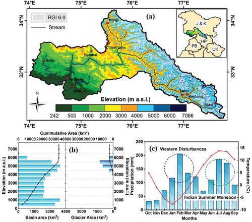
The Chenab River is a fourth-order basin of the great Indus River system, located in the foothills and very high, rugged mountains of the western Himalayas. The major part of the basin lies in the Indian Territory, whereas its lower part and outfall (into the Indus basin) are situated in Pakistan. In India, this river passes through two states, Himachal Pradesh, and Jammu & Kashmir, covering an area of ~7873 km² and ~22,323 km², respectively. The upper part of the basin lies between Zanskar and Pir Panjal ranges, whereas the lower part lies between Dhauladhar and the outer ranges of the Himalayas (P. Singh, Jain, and Naresh 1997). The eastern Hindukush, Karakorum and western Himalayas contributed ~50% of the total water supply originates from snow and glacier melt (Winiger, Gumpert, and Yamout 2005).

The Chenab River formed on the confluence of two streams, namely Chandra and Bhaga at Tandi, located in the Lahaul-Spiti district of Himachal Pradesh, India (Figure 1). These streams arise from snowfields on the opposite sides of the Baralacha Pass at an elevation of ~4900 m above sea level (a.s.l.) (P. Singh, Jain, and Naresh 1997). The CRB is elongated in shape and covers an area of 30,370 km². The total length of the Chenab River is approximately 974 km (Luqman et al. 2018), and it feeds several irrigation canals. The elevation of the basin varies widely from ~242 to 7066 m a.s.l., with an average of 2900 m a.s.l. However, the river gradient is excessively steep at its source and gradually decreases downstream. Additionally, the land use pattern of the basin involves forest and agriculture at an elevation of ~2500 m a.s.l., whereas higher elevation features subalpine and alpine conditions (Rao et al. 1997). The basin covers 2645 $\mathrm{k}{\mathrm{m}}^2$ of glaciers area, which mainly starts from an altitude of ~4000 m a.s.l. (RGI Consortium 2017).

Furthermore, the CRB lies in the boundary between two large-scale circulation patterns, i.e., the western disturbances and Indian summer monsoon system (Shekhar et al. 2010). Additionally, this basin is not only controlled by precipitation, but by changes in temperature also. For example, the climate of this basin varies from hot and moist, i.e., tropical, in the lower valley to cold temperatures at ~2000 m a.s.l. (Rao et al. 1997). Therefore, we have selected this basin for understanding the variability of meteorological variables and also the conflicting signals of climate change.

Figure 1. (a) Location map of the Chenab river basin and its location in India showing the altitude variation, drainage pattern, and glacier boundaries, (b) hypsometric curve of the basin and glacial area, and (c) mean monthly total precipitation and air temperature of ERA-5 reanalysis data extracted over the study area

2.2 Data used

2.2.1. MODIS snow cover products

In the present study, the MODIS daily snow cover products (SCPs) version 6 (V6) of Terra (MOD10A1) and Aqua (MYD10A1) were utilized over the study area from 1 January 2001 to 31 December 2017. We have selected the latest version of MODIS SCPs rather than the previous version 5 (V5) because Zhang et al. (2019b) found that V6 has higher accuracy than V5. The datasets were obtained from the NASA Earth data gateway customize service (https://search.earthdata.nasa.gov) with sinusoidal projection at 500-m grid resolution. The CRB comes under the MODIS tile number h24v05, i.e., horizontal 24 and vertical 5. For the observation period, a total of 6144 images for Terra and 5645 for Aqua were utilized while 65 and 15 images for Terra and Aqua were missing, respectively. Detailed information of MODIS SCP’s retrieved-snow-mapping algorithm is available at Riggs, Hall, and Roman (2016).

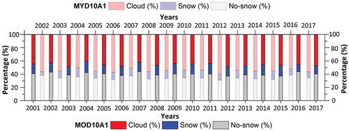
These data sets contain seven parameters (i.e., Normalized Difference Snow Index [NDSI] snow cover, raw NDSI, basic Quality Assessment [QA], algorithm flags QA, snow albedo, orbit pointer, and granule pointer) in Hierarchical Data Format (HDF). The NDSI snow cover parameter of both the sensors was used for snow cover mapping and monitoring. For this, we have used the global value of the NDSI threshold 0.4, which is still recommended (Riggs, Hall, and Román 2017; Riggs, Hall, and Roman 2016). The mean yearly percentage of the total geographical area, estimated for three new classes (i.e., cloud, snow, and no-snow) obtained from 9-standard MODIS classes (i.e., NDSI snow cover, Missing data, No decision, Night, Inland water, Ocean, Cloud, Detector saturated, and Fill). Overall, the mean cloud cover percentage of the total basin area in Aqua (54.9%) has accounted for 20.9% higher coverage than the Terra (45.4%) during the study period (Figure 2).

Figure 2. Mean annual percentage of the total geographical area calculated for cloud, snow, and no-snow classes during 2001–2017 for MOD10A1 (lower group) and 2002–2017 for MYD10A1 images (upper group)

2.2.2. Landsat-8 OLI satellite images

Due to scarcity of ground observations, numerous authors have used different high-resolution satellite data for validating the cloud gap-filled MODIS SCPs over various regions of the Himalayas (Hasson et al. 2014; Stillinger et al. 2019). Therefore, we have considered the Landsat-8 Operational Land Imager (OLI) images to validate the MODIS SCPs over the study period (2013–2017). A total of 47 cloud-free images were acquired (Path-147 and Row-38) from the United States Geological Survey (USGS) EarthExplorer, which is available at 30-m grid resolution and 16-day temporal scale (Table 1).

Table 1. Details of the Landsat-8 OLI data used for validation of the daily cloud-free MODIS SCA, from October 2013 to September 2017

Year	Date of image acquisition (DD/MM/YYYY)
2013	18/04/2013; 20/05/2013; 05/06/2013; 25/09/2013; 27/10/2013; 28/11/2013
2014	15/01/2014; 16/02/2014; 20/03/2014; 21/04/2014; 07/05/2014; 08/06/2014; 10/07/2014; 11/08/2014; 28/09/2014; 30/10/2014; 15/11/2014; 01/12/2014
2015	18/01/2015; 23/03/2015; 24/04/2015; 27/06/2015; 30/08/2015; 15/09/2015; 01/10/2015; 17/10/2015; 02/11/2015; 04/12/2015
2016	05/01/2016; 22/02/2016; 26/04/2016; 12/05/2016; 13/06/2016; 03/10/2016; 19/10/2016; 06/12/2016
2017	23/01/2017; 24/02/2017; 12/03/2017; 13/04/2017; 15/05/2017; 04/09/2017; 20/09/2017; 06/10/2017; 22/10/2017; 07/11/2017; 09/12/2017

2.2.3. ERA5-land reanalysis data

ERA5-Land is a global reanalysis dataset covering a period from 1981 to the present at 0.1º $\times$ 0.1º grid resolution with a monthly temporal scale. ERA5-Land provides a consistent view of the water and energy cycles at the surface level during several decades (C3S 2019). The performance of ERA-5 datasets were evaluated against the observed gridded datasets from the India Meteorological Department by Mahto and Mishra (2019), who reported that the ERA-5 performed better than other reanalysis products, thus it can be used for hydrological modeling over India. In this study, the total precipitation (${\mathrm{P}}_{\mathrm{t}}$), air temperature (${\mathrm{T}}_{\mathrm{a}}$), wind speed ($u$), and net shortwave radiation (SWN) were acquired in order to identify the influence of these variables on the spatial and temporal SCA over the CRB during two separate periods, i.e., 1981–2017 and 2001–2017.

2.2.4. Digital elevation model (DEM)

In this study, the void-filled Shuttle Radar Topography Mission (SRTM) digital elevation model (DEM) version 3.0 (~90 m spatial resolution) (Jarvis et al. 2008) was used to assess the topographical effect on SCA variation. The SRTM DEM was interpolated to the MODIS SCP’s spatial resolution of 500 m using the bilinear interpolation technique (suggested by Lopez-Burgos, Gupta, and Clark 2013). Vertical absolute and relative height error of the DEM was described to be less than $\pm$16 and $\pm$ 6 m respectively, while the circular absolute and relative geolocation error was $\pm$ 20 and $\pm$ 15 m, respectively, at a 90% confidence level (Farr et al. 2007; Rabus et al. 2003).

2.3 Methodology

2.3.1. Cloud removal methodology

To overcome the cloud gaps in the daily MODIS SCPs, we have selected and applied rigorous non-spectral cloud removal techniques over the extracted study area (Figure 4). The implemented methodology is a combination of high accuracy (> 90%) cloud reduction methods that are introduced by (Gafurov and András 2009; Wang et al. 2014) and partially adopted by (Parajka et al. 2010; Hasson et al. 2014; Paudel and Andersen 2011; Tran et al. 2019). These studies presented effective cloud removal techniques with the consideration of topographic and seasonal variability over the different regions. While these studies did include numerous cloud-gap filling steps in which each successive step reduced more cloud coverage, they also introduced a high probability of information loss (Gafurov and András 2009; Hasson et al. 2014). Therefore, we have produced a trade-off between cloud removal and information loss while considering the composite methodology of five different methods. The brief descriptions, theoretical accuracy, and functionality are discussed below.

The first step merged the MODIS Terra and Aqua images of the same day in order to minimize the short-term persistent cloud cover. We replaced the cloud pixels of the Terra image with the same day cloud-free pixels of the Aqua image by considering the Terra snow product as the primary image. This was done because the Terra image had experienced relatively less cloud coverage and had higher accuracy than the Aqua product (Hall et al. 2019). This step preferred more accurate and adequate snow cover than either observation could provide (Terra and Aqua). This may have occurred due to a short time difference (~3–4 h at the Equator) between these two sensors (Gafurov and András 2009).

The second step comprised the replacement of present-day cloud-pixels with a combination of two successive images (two forward and two backward). As for the temporal filling, three different temporal iterations were applied sequentially for snow and land pixels. In the first iteration, if both backward (t $-$ 1) and forward (t $+$ 1) images observed the same class (i.e., snow or no-snow) for the corresponding cloud pixel of the present image, then the cloudy pixel would be replaced by that class. Then, the second iteration applies a similar logic using images (t $-$ 1) and (t $+$ 2), followed by the third iteration using images (t $-$ 2) and (t $+$ 1). Here, we assumed that no snowmelt or snowfall occurred during the spans of different temporal iterations (Lopez-Burgos, Gupta, and Clark 2013). Moreover, the probability of rapid snowmelt was low because the present-day cloudy pixels limit the incoming shortwave radiation and diffuse the longwave radiation (Gafurov and András 2009). However, these assumptions showed significant disagreement in the transition zones as well as the transitional period. These changes were mainly attributed to the varying sun solar angle (Kahl, Dujardin, and Lehning 2019; Järvinen and Matti 2013), wind blow (Mott, Vionnet, and Thomas 2018), and avalanche events (Valero et al. 2018). These effects of sub-daily variation were not taken into account for this step due to the unavailability of sub-daily scale observation.

In the third step, the particular cloud cover pixel was replaced by the information from the eight nearest neighbor pixels, elevation, and aspect of the surrounding pixel. This method is explained by Gafurov and András (2009) and modified by Lopez-Burgos, Gupta, and Clark (2013). For the spatial filtering, we considered the two iteration processes sequentially for a 3 $\times$ 3 moving window in order to reduce the cloud cover. Also, numerous studies have suggested that this window size is optimal for cloud gap-filling (Gurung et al. 2011; Brooks, Wynne, and Thomas 2018; Chen et al. 2020). The first iteration removes a cloudy pixel; if any of this direct laying eight neighboring pixels covered by snow and their elevation was lower than the cloudy pixel with the same orientation, the cloudy pixel was assigned as a snow pixel. Also, if five out of eight neighboring pixels of the cloudy pixel showed snow/no-snow and a cloud pixel elevation was higher/lower from the minimum/maximum adjacent snow/no-snow elevation, then the cloudy pixel was reclassified as a snow/no-snow pixel.

In the fourth step, the regional snowline mapping approach (Parajka et al. 2010) utilized the aspect-wise elevation information to identify the snow/no-snow pixels correctly. For this, the cloudy pixels were assigned as snow or no-snow-based on their elevation, which was compared with the mean elevation of all the snow (${\mu }_s^h$) or no-snow (${\mu }_{ns}^h$) pixels in each aspect. The assumption of this filter is that at least 70% of the cloud-free pixel (Gafurov and András 2009) was present in a particular aspect; otherwise, this step would be skipped. In this approach, if the elevation of the cloudy pixel was above, the ${\mu }_s^h$ was classified as snow, and if the elevation was below, the ${\mu }_{ns}^h$ was assigned as no-snow. However, there would be no change in cloud pixels between the ${\mu }_s^h$ and ${\mu }_{ns}^h$ because the maximum uncertainty occurred in this transitional zone (Wang et al. 2009).

Although most of the cloud pixels were eliminated using the above-mentioned steps, additional remaining cloud pixels were also removed using a multi-day backward replacement method (Wang et al. 2014). In this approach, the cloud pixels on a current-day image were replaced by the cloud-free pixels of the previous day image and continuing until all the cloud pixels were removed. However, if the cloudy pixels were replaced by cloud-free pixels of a more extended previous-day image (i.e., cloud persistence continued), then the uncertainty of those pixels was increased.

Overall, the sequence of each subsequent step was considered based on their accuracy and their assumptions for cloud removal. Moreover, the combination of these steps was applied, and their outcomes were validated with the accuracy assessment methods.

2.3.2. Validation of methodology and their accuracy assessment

The best way to validate the composite cloud removal methodology was based on the in-situ measurement or ground truth data. However, the unavailability of continuous records and scarce measurement locations limited the validation with observatory data in the CRB. Therefore, the adopted methodology was validated using the indirect method suggested by Gafurov and András (2009) as well as high-resolution satellite data (Figure 4).

In the first (indirect) approach, a total of 186 images (157 belonging to Terra and 29 to Aqua) with less than 2% cloud cover from standard MODIS SCPs during the 17-year study period were utilized and filled with other dense cloud covered images. Then, the cloud-free images could be considered as “ground truth” observations for the corresponding cloud-filled images. Numerous authors have considered different sets of images for validation (Parajka and Blöschl 2008; Paudel and Andersen 2011; Dariane, Khoramian, and Santi 2017). Based on this, we selected a large number of images in order to better understand the accuracy of the composite methodology. However, the accuracy assessment results depended on the selection of the cloud-free images and their numbers in each month because of the snow cover condition variation in each month of the year. After applying the composite cloud removal methodology to the artificially generated cloud-covered images, we compared them with the corresponding cloud-free images. However, the first step (the combination of Terra and Aqua SCPs) was not validated due to the cloud cover differences between these two satellite images being very low within one day (Gafurov and András 2009). Further, the accuracy of the methodology was calculated by assessing the number of pixels reclassified correctly (i.e., snow to snow and no-snow to no-snow) and the number of pixels that was misclassified (i.e., snow to no-snow and no-snow to snow). Additionally, the overall accuracy was estimated by the percentage of correctly reclassified pixels to the total reclassified pixels in each image.

Second, for the validation method based on the high-resolution satellite data, the Landsat-8 OLI images were used to extract the snow region for the period 2013–2017. A total of 47 images of the different months were considered for the area comparison with corresponding cloud-free MODIS images. Therefore, binary snow cover maps were generated based on the reflectance bands (bands 3 and 6) of the Landsat satellite data with a threshold of NDSI [(band 3 $-$ band 6)/(band 3 $+$ band 6)] > 0.4, and the reflectance in band 5 (near-infrared) was > 0.11 for avoiding the water body. Then, we extracted the common snow-covered region from both datasets (MODIS and Landsat images) and compared them. Moreover, the relative error and mean absolute difference between these two datasets were calculated in order to assess the agreement (Hasson et al. 2014).

2.3.3. Snow cover indices

To investigate the snow cover change, one of the most popular indexes, i.e., Snow Cover Duration (SCD) was derived using the generated MODIS daily cloud-free images over the study period. The SCD is widely used in several studies to understand the interannual variations. Additionally, certain other indexes were estimated from the Snow Depletion Curves (SDCs), utilized by Dariane, Khoramian, and Santi (2017). The SDC was extracted by plotting the daily time-series of the SCA over the basin from September 1 to August 31. Hence, for the CRB, a total of 16 SDCs were obtained, one for each year. However, a five-day moving average of the SDC was also used to reduce the short-term snow cover variation. The details of the indexes used in this study (Figure 3) are explained as follows:

Figure 3. Conceptual diagram showing the snow depletion curve and defined snow indexes using daily cloud-free SCA between 1 September 2007 (Day-1) and 31 August 2008 (Day-366)

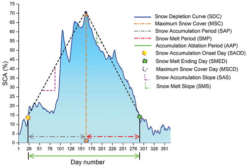
• Snow Accumulation Onset Day (SAOD): Considered as the day number from which snow accumulation started. The SAOD was estimated when the SCA exceeded 15% and remained above 15%. However, the shift in SAOD mainly occurred due to the precipitation and temperature changes.

• Snow Melt Ending Day (SMED): Considered as the day number that snow storage in the study area was depleted. The SMED was calculated when the SCA dropped below 15%, and was dependent on the amount of snow stored in the winter season, variability in solar radiation, and $T_a$ during the summer season.

• Accumulation-Ablation Period (AAP): Considered as the difference between the SAOD and SMED periods. It denoted the period of hydrological processes (snowfall and snowmelt) carried out in the basin.

• Maximum Snow Cover (MSC): Considered as the maximum extent of snow cover observed in a year. This index was mainly used to indicate the snow storage in the basin for that particular year.

• Maximum Snow Cover Day (MSCD): Considered as the day which MSC occurred.

• Snow Accumulation Period (SAP): Considered as the period from the SAOD to the MSCD.

• Snow Melt Period (SMP): Considered as the period between the MSCD and SMED. The SMP indicated the time taken by the snow stored in the basin to be depleted.

• Snow Accumulation Slope (SAS): Considered as equal to the ratio of MSC to SAP. SAS denoted the rate at which snow accumulation reached its maximum extent (i.e., the slope of the rising limb).

• Snow Melt Slope (SMS): Considered as the ratio of maximum snow cover extent (MSC) to the corresponding SMP. SMS was defined as a melting rate (i.e., the slope of the falling limb).

2.3.4. Statistical analysis

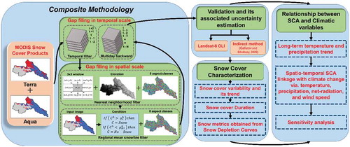
For the statistical analysis, the non-parametric Mann-Kendall (MK) trend (Mann 1945) and Sen’s slope estimator method (Sen 1968) were applied in monthly, seasonal, and annual time-series data of SCA and meteorological variables. Sen’s slope provides the rate of change over time-series data, whereas the MK test includes the monotonically increasing or decreasing trend. These trend detection methods are widely accepted in hydrology and meteorology time-series studies (Hamed 2009; Deng et al. 2018). The relationships of SCA with climatic variables were performed based on the Pearson correlation coefficient (R). Moreover, the daily MODIS SCA was classified into four seasons, i.e., December–January–February (DJF), March–April–May (MAM), June–July–August (JJA), and September–October–November (SON) in order to characterize the snow cover distribution in seasonal scale. Figure 4 shows the graphical representation of the overall workflow followed, including the cloud gap-filling composite methodology and the relationships between SCA and climatic variables.

Figure 4. Overall workflow of the methodology and analysis structure

3. Results

The present study produced cloud-free daily snow cover imagery using standard MODIS daily SCPs (Terra and Aqua) from 2001 to 2017. Here, we used preexisting techniques by considering only higher accuracy data (> 90%) for cloud removal. Moreover, the obtained results were validated by simulating the Gafurov and András (2009) method, and Landsat derived snow cover extent. Then, the generated cloud-free images were used to monitor the snow cover variability, dynamics, and its linkage with meteorological variables.

3.1 Validation of the cloud-free MODIS snow cover product

Firstly, the accuracy assessment was analyzed over 186 cloud-free MODIS images (157 for Terra and 29 for Aqua) by the indirect method. Several authors previously used the adopted methodology for accuracy assessment. The minimum, maximum, and mean accuracy achieved on images were 84.1%, 98.2%, and 93.1%, respectively, for the 157 Terra images, and 81.3%, 97.1%, and 91.3%, respectively, for the 29 Aqua images. The overall mean accuracy of the selected images (186 images) indicated higher efficiency in step-2 while lower in step-5 (Table 2). This may have occurred due to the longer time of backward image involvement which increased the persistent cloud days and produced uncertainty of the land features.

Table 2. Accuracy assessment of 186 images calculated for each step (from step 2 to 5) of the cloud removal methodology

Steps	Minimum	Maximum	Mean	Standard deviation	Kappa coefficient
2	89.1	98.3	94.2	1.21	0.91
3	86.3	96.6	93.3	1.65	0.86
4	84.3	97.6	94.1	1.78	0.83
5	81.2	94.5	89.8	1.61	0.81

The mean monthly accuracy of the selected images and their deviations were analyzed using the adopted methodology. Results indicate that the efficiency started decreasing from January (94.3%) and attained its minimum in July (90.5%) (Figure 5(a)). This may have occurred due to the variability of SCA being lower in the winter period as compared to other seasons (Gutzler and Rosen 1992). However, a lower accuracy was also observed in the transitional months, i.e., June, July, October, and November compared to other months. Similar results have been demonstrated by Li et al. (2019b) over the Tienshan Mountains using snow depth data. Moreover, a higher deviation was highlighted in July (1.9%). This could possibly be due to the monsoonal period, which may create a higher variation. The overall mean efficiency was obtained by about 92.8 $\pm$ 1.6%, with a kappa coefficient of 0.85 over the study period.

Figure 5. (a) Mean monthly accuracy of MODIS SCA using indirect method and (b) relative error between MODIS and Landsat SCA. The vertical line and bars represent the deviation and number of images, respectively, used for accuracy assessment

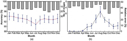
The second approach of cloud-free MODIS data validation included the area comparison between MODIS cloud-free images and Landsat snow cover extent over 2013–2017 (47 images). Validation results show that the mean absolute difference (MAD) between Landsat and MODIS SCA was approximately 2.4%, while the relative error ranged from −0.3% to 39.2%, with an average of 9.2% (Figure 5(b)). The estimated results indicate that the MODIS snow cover attained maximum overestimation in August (32.9%) and minimum in March (0.0%). Several authors have also reported an overestimation of MODIS snow cover with Landsat in different regions (Hasson et al. 2014; Tang et al. 2012). However, the underestimation was only slightly observed in January (0.1%). Besides, the MODIS cloud-free snow cover showed a higher correlation (R $=$ 0.99, p < 0.001) with Landsat data under clear sky conditions.

3.2 Effectiveness of the methodology

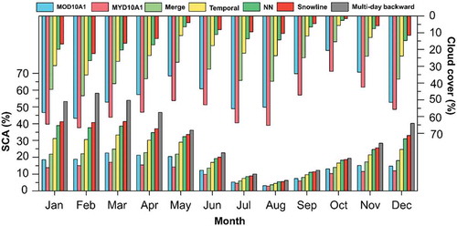
In this study, the effectiveness of individual steps was analyzed over the 17 years of data in order to demonstrate the amount of cloud removal and associated uncertainties. In standard SCPs, the percentage of cloud cover was higher in July and August and lower in October and May (Figure 6). This higher cloud obstruction might have occurred due to the influence of south-west summer monsoon, while the minimum obstruction may have been caused by the transition of the season (Padma Kumari and Goswami 2010). The mean cloud cover percentage of the basin area in standard MODIS Aqua was 20.9% higher than Terra; however, the mean SCA of Aqua was 30.6% less as compared to Terra SCP. This may have occurred due to the diurnal cycle of cloud cover that varies as well as increases throughout the day (Shang et al. 2018).

In the first step, the combination of Terra and Aqua snow products reduced the mean cloud cover from ~45.4% (Terra) and ~54.9% (Aqua) to 33.9% (combined products) of the total geographical area. However, the mean SCA was increased from 14.5% (for Terra) and 11.1% (for Aqua) to 16.2%. Overall, a five-step composite methodology reduced mean cloud cover by 33.9% (step-1), 20.4% (step-2), 13.4% (step-3), 8.3% (step-4) and ~0.0% (step-5). However, the mean SCA also progressively increased by 16.2%, 21.3%, 25.1%, 28.5%, and 33.6% in each subsequent step. However, in the last step, 30 previous-day images were used to remove almost all cloud pixels for the whole study area. This step removed the mean cloud cover from 8.3% (fourth step) to 5.1% (using first previous-day), 2.2% (using second previous-day), 1.8% (using third previous-day), and ~0.0% (using 30 previous-day images). This step considerably increased the mean SCA during the snow accumulation (December to March) and had no significant changes in the ablation season (July to September).

Figure 6. Month-wise progressive improvement obtained by the five different consecutive steps. The results are presented as mean SCA and cloud cover of the total study area during 2001–2017

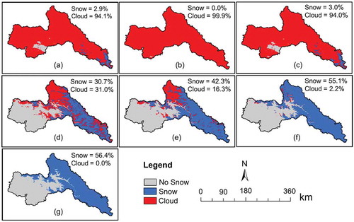
The performance of each subsequent step (from 1 to 5) for cloud removal was observed on a randomly selected date (12 March 2012), as shown in Figure 7. The standard Terra SCP observed 94.1% cloud cover (Figure 7(a)), whereas the Aqua satellite observed 99.9% of cloud coverage (Figure 7(b)) after a time difference of ~3 h. Obliviously, this percentage change in cloud cover reflected the continuous cloud movement dynamics. The implementation of the first step (combination of Terra and Aqua) removed 0.1% cloud cover from Terra and 5.9% from Aqua, while a total of 94.0% cloud cover remained (Figure 7(c)). The second step removed 63.0% cloud cover, while 31.0% remained (Figure 7(d)). However, the cloud coverage for the previous two, and the next two days was observed at 13%, 71%, 19%, and 46%, respectively. The third step removed 14.7% cloud cover, and 16.3% remained (Figure 7(e)). Although this step removed less cloud cover, it should still be considered as part of methodology due to its high accuracy and further minimization of the overall error. Many authors reported that the neighboring pixels method attains low error (Gafurov and András 2009; Tran et al. 2019). The fourth step, based on a regional snow line, removed 14.1% cloud cover and 2.2% remained (Figure 7(f)). Finally, the last step removed the remaining 2.2% cloud cover using a multi-day backward replacement approach (Figure 7(g)).

Figure 7. Cloud cover percentage of the randomly selected image and produced daily cloud-free image after implementation of the five steps on 12 March 2012. (a) Terra; (b) Aqua; (c) Combination of Terra and Aqua images; (d) Adjacent temporal combination; (f) Nearest neighborhood; (e) Regional mean snow line; and (g) Multi-day backward replacement

3.3 Uncertainty associated with cloud gap-filling techniques

In this study, the standard MODIS SCPs were used as observational data; however, all observational data have some inherent uncertainty. These inherent uncertainties are usually associated with the larger solar zenith angles, which can reduce the accuracy of the product (Li, Xingong, and Xiao 2016). Additionally, there are other uncertainties associated with the cloud gap-filling algorithm because of the different band considerations in Terra (band 6) and Aqua (band 7) for the NDSI algorithm (Hall and Riggs 2007). Moreover, the MODIS snow product has an advantage for large areas; however, the accuracy of the single-pixel can be influenced by different variables, i.e., acquisition angle, acquisition time, topographic effect, and land cover (Matiu, Jacob, and Notarnicola 2020). These factors lower the accuracy, especially in the starting and ending of the snow season. Therefore, the last multi-day backward replacement filter was used to provide reasonable estimation when averaged over the more extended periods. Hence, special consideration should be given for the daily value of snow cover pixels during monsoon season.

3.4 Snow cover variability

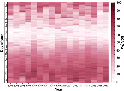
After a satisfactory assessment of the methodology efficiency, the generated new daily cloud-free MODIS snow cover images were used to understand the intra-annual and inter-annual variability of snow cover over the CRB. Daily distributions of the SCA for each date from 1 January 2001 to 31 December 2017, depicting the annual cycle are shown in Figure 8. The sequence of daily images indicates that the major snowfall events and growth/shrink of snowfall period over one year changes from decade to decade. It also suggests that the snow cover extent is highly variable within the observation period, further leading to a shift in the snowfall season.

Figure 8. Daily cloud-free snow cover area of the Chenab river basin from 1 January 2001 to 31 December 2017

The annual evolution of snow cover during 2001–2017 was analyzed for the entire basin (Figure 9). The mean yearly SCA was 33.6% of the total geographical area. The mean annual minimum and maximum SCA were observed in 2016 (27.0%) and 2015 (37.5%), respectively. The maximum SCA mostly occurred in February except for the years 2001, 2006, 2007, 2009, and 2017; while the minimum SCA was mostly observed in August except in 2011. Previous studies have also suggested that the maximum and minimum SCA occurred in February and August, respectively, for the western Himalayas (Kour, Patel, and Krishna 2016a; Kripalani, Kulkarni, and Sabade 2003); thus this coincided with our results. Also, Dimri et al. (2015) have reported that the major snowfall events occur during December, January, and February were mainly influenced by the western disturbances over the Himalayas. In general, if the maximum SCA occurred in January, this would likely result in a higher rate of melting due to increasing the ablation period and directly contributing to the river system (Barnett, Adam, and Lettenmaier 2005).

Figure 9. Mean annual and monthly minimum and maximum SCA per year over the Chenab basin from 2001 to 2017

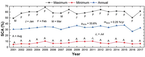
For the observation period, the mean monthly SCA was more persistent in February (58.2%), followed by January (54.5%), and March (54.0%); while the minimum SCA was observed in August (6.2%), followed by July (10.1%), and September (13.9%). The transitional months of September, October, and November showed the highest inter-annual SCA variability with a coefficient of variance (Cv) of 0.27, 0.30, and 0.29, respectively, whereas March (Cv = 0.07) and April (Cv = 0.07) experienced the least variability and were relatively stable.

To evaluate the significant change in snow cover trend, a non-parametric MK and Sen’s slope test were performed on monthly, seasonal, and annual time scales in three separate periods, i.e., 2001–2017, 2001–2009, and 2009–2017 (Figure 10). It should be noted that a statistical trend for a shorter period than these should be treated carefully. Although the result shows an increasing trend of SCA for the periods 2001–2017 and 2001–2009, it has been slightly decreasing since 2009 and was statistically insignificant. Therefore, an insignificant increasing trend of SCA was observed at a rate of 0.25% $\mathrm{y}\mathrm{r}-1$ for the entire period. Moreover, the SCA increased or was stable from January to April during each selected period. This may indicate that the snow accumulation period has changed or is shifting in terms of the seasonal snow cover (M. K. Singh, Thayyen, and Jain 2019). The reduction in mean annual SCA was increased by ~6.8% during 2001–2009; however, recently, it was decreased by ~1.5% of the total basin area during 2009–2017. Moreover, the maximum SCA was reduced (about 10.2%) in SON and was increased (about 1.5%) in DJF during 2009–2017.

Figure 10. Trend analysis of the mean monthly, seasonal, and annual SCA of the Chenab basin during three distinct periods: 2001 to 2017, 2001 to 2009, and 2009 to 2017

3.5 Snow cover depletion curve indexes

The Snow Depletion Curve (SDC) was used to extract the different indexes for the entire basin to understand the properties of the snow accumulation-ablation season. Results indicate that the MSC trend was decreasing (−0.12$\mathrm{\%}\mathrm{y}\mathrm{r}-1$) for the entire area. Moreover, the SAP was shortened (−1.44 day $\mathrm{y}\mathrm{r}-1)$, resulting in stable or no trend of the SAS, which is the ratio of MSC to SAP. In contrast, SMP was elongated by about one day per year with decreasing SMS (−0.004). However, the MSCD was shifting backward at the rate of about one day per year. The trend of SAOD indicated that the snow accumulation started one day earlier, while that of the SMED showed that the average snowmelt season ended one day earlier in each year. Overall, the AAP indicated a decreasing trend at the rate of −0.92 day $\mathrm{y}\mathrm{r}-1$; however, the SAP decreased and SMP increased at the rates of −1.44 and 1.19 day $\mathrm{y}\mathrm{r}-1$, respectively. All indexes showed insignificant trends (p < 0.05) during the study period.

3.6 Snow cover days (SCDs)

The pixel-wise Snow Cover Days (SCDs) for each year were calculated based on cloud-free daily snow cover images. The average SCD of the basin was ~122 days during the study period. A 17-year mean SCD was classified into six subsequent classes (Figure 11). The SCD less than 60 days covered the majority of the basin, ~45.0%, which was considered as unstable SCA. The other classes, such as 60–120, 120–180, 180–240, and 240–300 days, occupied areas of about 8.4%, 11.3%, 14.6%, and 10.5%, respectively. However, the majority of mountain peaks and glaciers were covered with SCDs above 300 days, with an area of 10.5%. In addition, more SCD values were observed in the higher elevations of the basin (above 5000 m a.s.l.), which received higher snowfall in comparison to the lower reaches. This region attains the majority of the CRB glaciers, which have relatively persistent snow as compared to the mid-lower and lower elevations. This indicates that the SCD was minimum for areas near 2200 m elevation, and the duration of snow cover became shorter.

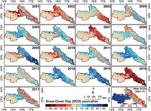
The spatial distribution of SCD anomalies (deviation from the 17-year mean) of each year is illustrated in Figure 11. We observed a relatively shorter SCD than the total mean in the years of 2001, 2002, 2003, 2016, and 2017, particularly in the year 2016 (23 days). In contrast, the years 2004, 2010, and 2013 were stable with the SCD being close to the mean. However, the rest of the years were considered as longer than the mean of the SCD, especially in 2015, which indicated that the SCD was 15 days longer than the mean. Randhawa, Rathore, and Ishant (2016) have found that the SCA reduced significantly during 2015–2016 in comparison to 2010–2014 in almost all basins of the Himachal Pradesh, western Himalayas.

Figure 11. Spatial distribution of SCD anomalies (deviation from the mean of the 2001–2017 period) per year from 2001 to 2017

3.7 Snow cover influence by topographic parameters

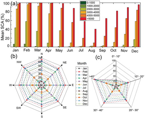
The topographical effect on SCA variations was investigated over six different elevation bands (elevation-wise), eight aspect classes (aspect-wise), and five slope classes (slope-wise) over the entire time-series of data (Figure 12). For this, the classified areas for each elevation zone were 21.5% for 0–1000 m a.s.l., 13.9% for 1000–2000 m a.s.l., 14.2% for 2000–3000 m a.s.l., 16.3% for 3000–4000 m a.s.l., 22.3% for 4000–5000 m a.s.l., and 11.7% for elevations over 5000 m a.s.l. of the total basin area, for which the mean SCA values were about 1.6%, 14.7%, 41.9%, 65.5%, and 84.6%, respectively (Figure 12(a)). Additionally, elevations above 4000 m a.s.l. covered 34% of the basin area, which included 97.5% of the core glacier area within the basin. However, the SCA for the period 2001–2017 showed an increasing trend at the rate of 0.78% $\mathrm{y}\mathrm{r}-1$, whereas a decreasing trend (−1.36 $\mathrm{\%}\mathrm{y}\mathrm{r}-1$) in SCA was observed during 2009–2017 for the elevations above 4000 m a.s.l. This decreasing trend of SCA in higher altitudes could have led to the negative glacier mass balance (Singh, Thayyen, and Jain 2019) and increase in streamflow (Lutz et al. 2014) observed in the recent decade. However, the overall SCA showed a decreasing trend from September to January, whereas an increasing trend was experienced from April to August, which is statistically insignificant above 4000 m a.s.l. It should be noted that the elevation zones between 4000 and 5000 m and above are likely to be most sensitive to climate change as most of the glaciers exist at these elevations, and a significant amount of snow cover remains throughout the year. Therefore, this change in SCA at higher elevations could have a major impact on glacier mass balance and regional water storage.

The SCA dependency on aspect-wise varied from location to location because precipitation was influenced by the function of aspect and prevailing wind direction. Therefore, the aspect values were classified as 7.3% for north (337.5–22.5°), 10.8% for northeast (22.5–67.5°), 10.7% for east (67.5–112.5°), 13.6% for southeast (112.5–157.5°), 17.5% for south (157.5–202.5°), 15.9% for southwest (202.5–247.5°), 12.5% for west (247.5–292.5°), and 11.7% for northwest (292.5–337.5°) of the total basin area (Figure 12(b)). It was found that the north and south directions experienced the maximum and minimum SCA in each month, respectively, with the highest occurring in February and lowest in August. By combining the elevation and aspect information, it can be concluded that aspect is not a strong limiting factor for snow persistence in the higher regions during the winter season. However, snowmelt becomes more relevant when the climatic condition is changed, or if solid precipitation is weaker in the higher elevations. The slope orientation of the basin has a relatively larger area in the south and southwest, and higher SCAs in the north (40.0%), northeast (35.0%), and northwest (38.9%) during all seasons were observed.

For quantitative snow cover distribution, the slope of the basin was classified into five different categories, i.e., 0–10°, 10–20°, 20–30°, 30–40°, and above 40°, which covered areas of 20.9%, 20.9%, 29.3%, 22.1%, and 6.8% of the total basin area, and mean SCA was observed at 17.5% 29.8%, 36.0% 42.1%, and 53.8% respectively (Figure 12(c)). The basin experienced a maximum and minimum SCA above 40º and 10–20º, respectively, in all months; however, was highest in February and lowest in August. This could be related to the solar radiation being the largest and smallest on steep south-facing and north-facing slopes, respectively. However, the flatter terrain of lower elevations receives more solar radiation than the steeper slopes. Therefore, the SWN can be influenced by the change in slope and direction, which tends to change in snowmelt (Seyednasrollah and Kumar 2014).

Figure 12. Mean SCA distribution from 2001 to 2017 in classified: (a) Elevation; (b) Aspect and (c) Slope of the Chenab basin

3.8 Relationship of SCA with climatic parameters

To investigate the possible mechanism of snow cover variability, the linkages between the snow cover and climatic variables, i.e., ${\mathrm{T}}_{\mathrm{a}}$, ${\mathrm{P}}_{\mathrm{t}}$, SWN, and $u$, were analyzed. The climatic variables were explained in two ways. First, the long-term spatiotemporal trend of ${\mathrm{T}}_{\mathrm{a}}$ and ${\mathrm{P}}_{\mathrm{t}}$ were analyzed during 1981–2017 to understand decadal changes, which were further linked to regional-scale climate variabilities. Second, the relationships between SCA and the climatic variables were established using Pearson’s correlation coefficient and regression analysis.

3.8.1 Temperature and precipitation analysis (1981–2017)

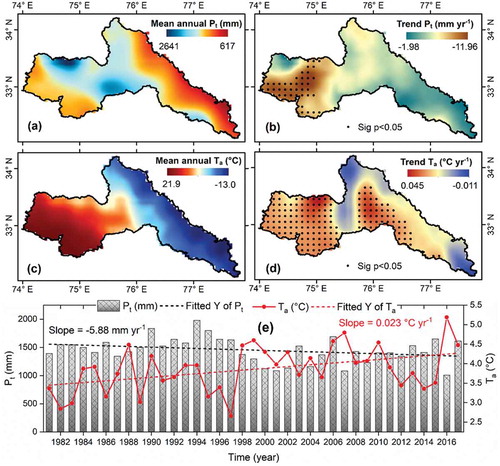
The annual trends of ${\mathrm{T}}_{\mathrm{a}}$ and ${\mathrm{P}}_{\mathrm{t}}$ were assessed for 1981–2017. Results showed a significant increase in mean annual ${\mathrm{T}}_{\mathrm{a}}$ at the rate of 0.023 ${ }^{\circ }\mathrm{C}\mathrm{y}\mathrm{r}-1$, while ${\mathrm{P}}_{\mathrm{t}}$ decreased at the rate of −5.88 $\mathrm{m}\mathrm{m}\mathrm{y}\mathrm{r}-1$ (Figure 13(e)). The maximum and minimum temperatures were observed in 2016 (5.19°C) and 1997 (2.66°C), respectively, with a mean value of 3.86°C. Relatedly, 2007, 2010, and 2016 were the warmest years in the Hindu-Kush Himalayan region for the period of 1901–2014 (Wester et al. 2019; Ren et al. 2017). Similarly, the mean maximum and minimum of ${\mathrm{P}}_{\mathrm{t}}$ were observed in 1994 (1978.4 mm) and 2016 (1007.7 mm), respectively, with a mean value of 1452.8 mm. Previous studies have reported that the snow/ice cover area decreased by 0.9% over the Himalayan region between 1990 and 2001 (Menon et al. 2010) due to aerosols. This reduction in snow cover can be supported by our study of the previous decade (1990–2001), which showed a decrease in ${\mathrm{P}}_{\mathrm{t}}$ (−60.5 $\mathrm{m}\mathrm{m}\mathrm{y}\mathrm{r}-1$, p < 0.05) due to a rise in ${\mathrm{T}}_{\mathrm{a}}$ (0.049${ }^{\circ }\mathrm{C}\mathrm{y}\mathrm{r}-1$over the study area.

Additionally, the spatial distributions of $\mathrm{T}\mathrm{a}$ (Figure 13(a,b)) and ${\mathrm{P}}_{\mathrm{t}}$ (Figure 13(c,d)) were observed using MK and Sen’s slope test. As identified visually, the rate of change in ${\mathrm{T}}_{\mathrm{a}}$ and ${\mathrm{P}}_{\mathrm{t}}$ varied from location to location. Bhutiyani, Kale, and Pawar (2007) have reported that the northwest Himalayan region has shown a significant rise in ${\mathrm{T}}_{\mathrm{a}}$ by about 1.6°C during the last century (1901–2001) and winter warming at a faster rate. Also, Jaswal and Prakasa Rao (2010) have highlighted significant increases in the maximum ${\mathrm{T}}_{\mathrm{a}}$ over the Kashmir region and the minimum ${\mathrm{T}}_{\mathrm{a}}$ over the Jammu region during 1976–2007. Furthermore, in this study, ${\mathrm{P}}_{\mathrm{t}}$ decreased in the southeast region of the CRB with an increase in ${\mathrm{T}}_{\mathrm{a}}$. However, both ${\mathrm{P}}_{\mathrm{t}}$ and ${\mathrm{T}}_{\mathrm{a}}$ increased in the northwest region with statistically significant values.

Figure 13. Spatiotemporal pattern of a) mean annual air temperature and its trend (b); c) total yearly precipitation and its trend (d); and e) linear relationship between annual temperature and precipitation, derived from gridded data during 1981–2017

3.8.2 Impact of climatic variables on SCA (2001–2017)

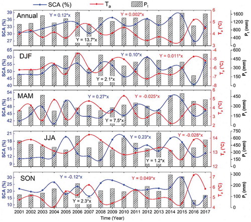
The linear relationships between SCA and climatic variables were performed on seasonal and annual data for the period 2001–2017 (Figure 14), and indicates that SCA has an inverse relation with ${\mathrm{T}}_{\mathrm{a}}$ and a direct relationship with ${\mathrm{P}}_{\mathrm{t}}$. Additionally, the mean monthly and annual ${\mathrm{T}}_{\mathrm{a}}$ of each year shows an increasing slope except for the MAM and JJA. However, with a higher increase in ${\mathrm{T}}_{\mathrm{a}}$, the snow cover in the later season (SON) decreased further. Another effect is that the liquid ${\mathrm{P}}_{\mathrm{t}}$ increased because ${\mathrm{P}}_{\mathrm{t}}$ occurred as rain in higher ${\mathrm{T}}_{\mathrm{a}}$ conditions; therefore, the SCA dynamics were affected. Moreover, the present study suggested that the rate of SCA attained a higher positive value in MAM as compared to DJF, while the ${\mathrm{T}}_{\mathrm{a}}$ rate increased in DJF as compared to MAM (decreasing). This may have occurred due to a shift in the seasonal cycle of climatic variables. A similar pattern was observed by numerous authors (P. Singh, Jain, and Naresh 1997; Kour, Patel, and Krishna 2016b; Anjum et al. 2019).

However, these trends are represented for a shorter period of time which cannot fully explain the SCA expansion. Winter ${\mathrm{P}}_{\mathrm{t}}$ and ${\mathrm{T}}_{\mathrm{a}}$ may be considered as key factors for the increasing SCA trends in the CRB and should be studied using more reliable high-altitude data. Also, Rathore et al. (2018a) have observed a rising trend of snow cover in all basins of the western and west-central Himalayan regions during 2004–2014, and Negi et al. (2017) have reported that the winter (November to April) mean ${\mathrm{T}}_{\mathrm{a}}$ was decreasing, and the number of snowfall days was increasing insignificantly in the northwest Himalayan region from 2001 to 2014. Furthermore, Gurung et al. (2011) have showed that snow cover trends for the western Himalayan region were positive for all seasons from 2000 to 2010. Immerzeel et al. (2009) have also reported an insignificant increasing trend of snow cover variation from west to east over the Himalayas between 2000 and 2008.

Figure 14. Linear variation of mean seasonal and annual SCA, air temperature, and precipitation from 2001 to 2017 over the Chenab basin

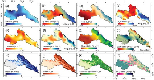
To evaluate the response of SCA and SCD with the climatic variables and energy flux, the spatio-temporal patterns of ${\mathrm{P}}_{\mathrm{t}}$, ${\mathrm{T}}_{\mathrm{a}}$, $u$, and SWN were assessed over the CRB for the period 2001–2017 (Figure 15). Results showed an increasing trend of ${\mathrm{P}}_{\mathrm{t}}$ with a rate of 21.2 $\mathrm{m}\mathrm{m}\mathrm{y}\mathrm{r}-1$ for the entire basin. Further, ${\mathrm{P}}_{\mathrm{t}}$ was found to increase less in the high mountain regions. This result is in good agreement with Dahri et al. (2016) and Rizwan et al. (2019). However, the $u$, ${\mathrm{T}}_{\mathrm{a}}$, and SWN rates were also substantially increasing for the low to medium clusters. The analysis demonstrates that the ${\mathrm{P}}_{\mathrm{t}}$ and SWN were increasing in the northeastern region of the basin; however, for ${\mathrm{T}}_{\mathrm{a}}$ and $u$, decreasing trends were observed. In contrast, decreasing trends of ${\mathrm{P}}_{\mathrm{t}}$ and SWN were observed in the central part of the basin along with the increasing trends of ${\mathrm{T}}_{\mathrm{a}}$ and $u$.

Additionally, the increasing ${\mathrm{T}}_{\mathrm{a}}$ reduces the SCDs and increases its deviation, which further leads to an earlier onset of snowmelt. This result was previously explained by Rathore et al. (2018b) over the CRB. Also, Shafiq et al. (2018) have reported that the maximum and minimum ${\mathrm{T}}_{\mathrm{a}}$ was decreased while the ${\mathrm{P}}_{\mathrm{t}}$ was increased in the Kashmir Valley, located in the northwest region of the Himalayas. Furthermore, the SCA variation was influenced by the energy and mass fluxes of the underlying surface. The regions with higher SCA reflect more solar energy with less absorption, which decreases the SWN over the area. Therefore, the SWN was higher in the snow-free region and lowered in the snow-covered region. Additionally, the small cluster of SWN was increasing over the region, whereas SCDs decreased. This may have occurred due to the spatial heterogeneity of the SCA and SCDs that varied from location to location. However, the increasing $u$ also helped to increase the mass fluxes, i.e., sensible and latent heat. Moreover, it may have affected the amount of sublimation/re-sublimation in the snow-covered region. Overall, the changing trends of these climatic variables help in understanding the influence of snow cover distribution and the onset of snowmelt.

Figure 15. Spatial pattern of annual (a, b) precipitation and its trend, (c, d) mean air temperature and its trend, (e, f) wind speed and its trend, (g, h) net shortwave radiation and its trend, (i) mean SCA, (j) mean annual SCD, (k) SCD standard deviation, and l) SCD trend over the study area during 2001–2017

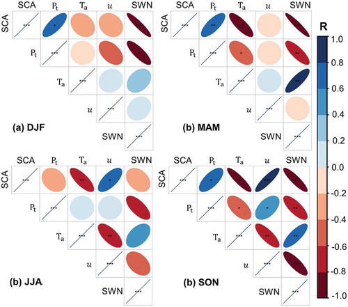
The inter-relationships between SCA, ${\mathrm{P}}_{\mathrm{t}}$, ${\mathrm{T}}_{\mathrm{a}}$, $u$, and SWN were calculated using Pearson’s correlation coefficient for the period 2001–2017 (Figure 16). Results indicate that ${\mathrm{P}}_{\mathrm{t}}$ showed a significant positive correlation with the SCA for all months except JJA over the CRB. This may be because the basin is predominantly influenced by the ISM, which is active during JJA and attains a majority of ${\mathrm{P}}_{\mathrm{t}}$ in the form of rain (Dahri et al. 2016). Similarly, a significant negative correlation was observed between SCA and ${\mathrm{T}}_{\mathrm{a}}$ throughout all months except for DJF. In these months, the ${\mathrm{T}}_{\mathrm{a}}$ shows a low variation (almost negative) as compared to the SCA. Additionally, the SWN was also found to be less negatively correlated with the SCA for the JJA; otherwise, it showed a significant negative correlation for the rest of the months. This can be evidence of the fact that the SWN usually reaches its maximum from June to July. However, the SCA started decreasing from June and reached a minimum value in August, which may have resulted in the poorer correlation. However, $u$ showed a significantly positive correlation with the mean SCA for the period June–November. Overall, the annual SCA showed a significant positive correlation (p < 0.05) with ${\mathrm{P}}_{\mathrm{t}}$ and $u$ and a negative correlation (p < 0.01) with ${\mathrm{T}}_{\mathrm{a}}$ and SWN over the basin. These interrelationships help to identify the contributing factors controlling the spatial and temporal distribution of the SCA. Therefore, a further study is recommended, so as to determine exact processes which could contribute to an increase in SCA across the basin.

Figure 16. Seasonal Pearson correlation coefficients between SCA, air temperature, precipitation, wind speed and SWN over the Chenab basin from 2001 to 2017

3.8.3 Sensitivity analysis

The sensitivity analysis was performed by developing a multiple linear regression model between dependent, i.e., SCA, and independent variables, i.e., ${\mathrm{P}}_{\mathrm{t}}$ and ${\mathrm{T}}_{\mathrm{a}}$, during 2001–2017 for the entire basin. The model showed a high correlation (R = 0.81, p < 0.001) between the variables. ${\mathrm{P}}_{\mathrm{t}}$ and ${\mathrm{T}}_{\mathrm{a}}$ were altered by$\pm$ 30% and $\pm$ 2°C, respectively. Results showed that the snow cover response to the warming temperature ($\pm$ 2°C) was very rapid, which reduced the SCA by $\mp$ 11%. In general, the snow cover showed a higher sensitivity to ${\mathrm{T}}_{\mathrm{a}}$, meaning that small changes in ${\mathrm{T}}_{\mathrm{a}}$ generated significant variation in the SCA. This obtained result was also highlighted by Rathore et al. (2018b) and Kour et al. (2016a). They found a strong connection between the ${\mathrm{T}}_{\mathrm{a}}$ and SCA variability over the CRB. Our result indicates that the increasing ${\mathrm{P}}_{\mathrm{t}}$ (in this case $\pm$ 30%) had little effect on the snow cover change ($\pm$ 6%); however, a strong influence occurred during the snow accumulation season. A similar result was demonstrated by Brown and Mote (2009) over the Northern Hemisphere (NH). Overall, this analysis suggests that the SCA is more sensitive to ${\mathrm{T}}_{\mathrm{a}}$; however, is less susceptible to ${\mathrm{P}}_{\mathrm{t}}$ during the melt season for the selected observational period.

4. Discussion

Information on spatial distribution and temporal dynamics of snow cover is crucial for understanding the hydrological system within the CRB. In comparison to other regions in the same latitude, the CRB in the western Himalaya is influenced by both ${\mathrm{P}}_{\mathrm{t}}$, i.e., ISM in summer and mid-latitude westerlies in winter (Shekhar et al. 2010). Furthermore, this region has the potential to be the “home to the largest capacity of hydropower project[s]” among all the basins in India (Thakur and Asher 2015). Therefore, seasonal snow cover monitoring at the basin scale is crucial in order to measure the water availability from snowmelt in the summer season. Thus, a reliable estimate of the spatio-temporal snow cover trend and its response to future climatic change is needed. However, ground observations are rare and temporally limited in the high mountainous region of the CRB. The high-temporal resolution of the MODIS instrument can overcome this limitation and provide an excellent opportunity to study the snow cover variability. The snow cover result of MODIS data was previously validated over different parts of the world (Hall and Riggs 2007; Gafurov and András 2009) within the Hindu-Kush Himalayas (Forsythe et al. 2012; Hasson et al. 2014) and also in the western Himalayas (Chelamallu, Venkataraman, and Murti 2014; Jain, Goswami, and Saraf 2008).

The higher accuracy (> 90%) methods were combined, and composite methodology was used to remove the cloud cover and maintain the overall accuracy of the selected MODIS snow product. The validation of the methodology suggested that the applied method substantially eliminated the cloud cover with high efficiency over the study area. However, it was also observed that the cloud gap-filling technique was unable to completely remove the clouds from the snow product because of the persistent cloud being longer than the temporal window size, as well as because of more significant cloud cover extent (Hasson et al. 2014). Therefore, the results suggest that the cloud percentage was higher during JJA. A similar pattern of higher cloud cover in the melt season compared to that of the accumulation season was reported by Maskey, Uhlenbrook, and Ojha (2011) over the central Himalayas. Therefore, the adopted methodology was limited during the respective season, especially for the high mountain glacierized region during the melt season. Still, the overall performance of the methodology was satisfactory in that the importance of gap-filling of cloud cover was highlighted, along with an improvement of SCA.

The variability of the SCA on the CRB was characterized by seasonal and annual changes, which varied with different elevation, slope, and aspect. The study shows that the snow cover has a heterogeneous distribution over the CRB with more variation in the northeastern region and less snow cover in the western region of the basin. The snow cover extent significantly decreased in the NH, especially in spring (Yeo, Kim, and Kim 2017). Satellite records indicate that during 1967–2012, the SCA reduced considerably, and the most significant change occurred in June (IPCC 2013). Rathore et al. (2018a) have also highlighted the higher variability of snow cover at the sub-basin scale in the Indus, Chenab, Sutlej, and Ganga basins during the accumulation period rather than the ablation. The overall trend of snow cover shows an increasing trend over the basin. However, Sahu and Gupta (2020) have also reported the SCA shrinking at the rate of 0.12% per year over the Chandra basin during 2001–2016. This inconsistency in results may be due to the temporal change in the MODIS snow product (8-day MOD10A2). Additionally, Kour et al. (2016a) have demonstrated that the SCA was significantly increased due to a significant increase in snowfall and a decrease in ${\mathrm{T}}_{\mathrm{a}}$ during 2000–2013.

The linear relationships between the SCA with the topographic parameters suggested that the SCA trend decreased in September–January for elevations above 4000 m a.s.l., while it increased in April–August. This pattern also was demonstrated by Kour, Patel, and Krishna (2016b). Additionally, the SCDs and nine snow indexes showed significant shifting movement in and shortening of the snow accumulation period over the basin. An early snow melting was also reported by Ayub et al. (2020) over the upper Indus basin.

Generally, the large interannual variability in snow cover in the CRB is the more striking feature (Rathore et al. 2018a; Kour, Patel, and Krishna 2016b), as well as its linkage with climatic variables and energy fluxes necessary for the future prediction and policy adaptation. This analysis shows that the region has experienced an increasing trend of SCA with a statistically significant increase in ${\mathrm{P}}_{\mathrm{t}}$ and ${\mathrm{T}}_{\mathrm{a}}$ during 1981–2017. In addition, there is a high positive correlation between the SCA and ${\mathrm{P}}_{\mathrm{t}}$, and a negative correlation with ${\mathrm{T}}_{\mathrm{a}}$. The northwest Himalayan region reported a substantial rise in air temperature by about 1.6°C during the last century (1901–2001) and winter warming at a faster rate (Bhutiyani, Kale, and Pawar 2007). IPCC (2013) have reported that the mean annual ${\mathrm{T}}_{\mathrm{a}}$ of the NH during 1983–2012 was considered as the warmest 30-year period of the last 1,400 years, and the results this study agree. Investigation at similar latitudes with longer records of ${\mathrm{P}}_{\mathrm{t}}$ (Rizwan et al. 2019) and ${\mathrm{T}}_{\mathrm{a}}$ trends (Bhutiyani, Kale, and Pawar 2010) have been observed. Additionally, results showed a significantly negative correlation of ${\mathrm{T}}_{\mathrm{a}}$ with the SCA. SWN directly affects the melt recharge and evaporation, which influenced the forest cover and hydrological system (Seyednasrollah and Kumar 2014).

Overall, our findings suggest that the SCA over the CRB is highly variable and is influenced by climatic variables as well as energy fluxes. Future research on the CRB may focus on the effect of changing SCA on snowmelt and streamflow efficiency and timing. This information could be helpful for informing water resource management if the SCA and SCD decrease.

5. Conclusions

The spatial characteristics and temporal dynamics of snow cover distribution were examined on the daily MODIS snow cover products (MOD10A1 and MYD10A1, version 6) in the CRB for the period 2001–2017 to understand the present state of the snow-cover regime. The period of the dataset is relatively short for the robust conclusion related to the long-term SCA changes and their behavior. Nevertheless, the data provide insight into the shortcoming changes in the SCA and assist in the continuous monitoring of hydrological processes. Results showed that the obtained cloud-free SCA observed high accuracy of ~92.8 ± 1.6%, with a kappa coefficient of 0.85 over the study period using an indirect method (Gafurov and András 2009). Additionally, the direct comparison between Landsat and MODIS SCA showed an overestimation (9.3%). However, a higher correlation (R = 0.99, p < 0.001) was observed with MODIS SCA under clear sky conditions. Moreover, the effectiveness of the methodology in each subsequent steps indicates that the mean cloud cover percentages were removed by 33.9%, 20.4%, 13.4%, 8.3%, and ~0.0%, respectively, and the mean SCA increased about 16.2%, 21.3%, 25.1%, 28.5%, and 33.6% respectively.

Therefore, after a satisfactory assessment of methodology efficiency and its uncertainties, the daily cloud-free snow cover images were used for intra-annual and inter-annual variability of snow cover over the CRB. Results demonstrated an increasing trend of SCA for the period 2001–2017 (at a rate of 0.25% $\mathrm{y}\mathrm{r}-1$), while the rate has been slightly decreasing since 2009 with statistically insignificant values. Furthermore, the SCD and nine other indexes were derived from the SDCs to evaluate the snow cover characterization, indicating that the SAP was shortened while the SMP was elongated by about one day per year. Moreover, the relationships between SCA and topographic parameters indicated that the overall SCA showed a decreasing trend from September–January, and an increasing trend from April–August above 4000 m a.s.l. However, these trends were statistically insignificant. The maximum and minimum SCA for all months were experienced in the north for the high-altitude/latitude (4000 m.a.s.l. and above) and south in lower-altitude/latitude (1000–2000 m.a.s.l.), respectively. An insignificant decreasing trend was observed in the elevations of 4000–5000 m a.s.l. (−1.36% $\mathrm{y}\mathrm{r}-1$) and above 5000 m a.s.l. (−1.19% $\mathrm{y}\mathrm{r}-1$) during 2009–2017, compared to the 2001–2009 period. This clearly indicates that the snow accumulation period has changed or is shifting in terms of the seasonal snow cover during the recent decade.

The linear relationship between SCA and climatic variables, as well as energy fluxes, were established to identify the possible influence of snow cover distribution and the onset of snowmelt. The analysis demonstrated that the ${\mathrm{P}}_{\mathrm{t}}$ and SWN were increasing in the northeastern region of the basin; however, ${\mathrm{T}}_{\mathrm{a}}$, and $u$ showed declining trends. In contrast, decreasing trends of ${\mathrm{P}}_{\mathrm{t}}$ and SWN were observed in the central part of the basin, whereas the trends of ${\mathrm{T}}_{\mathrm{a}}$ and $u$ were increasing. Overall, the annual SCA shows a significant positive correlation (p < 0.05) with ${\mathrm{P}}_{\mathrm{t}}$ and $u$, and a negative correlation (p < 0.01) with ${\mathrm{T}}_{\mathrm{a}}$ and SWN over the basin. Furthermore, a sensitivity analysis was performed, suggesting that the SCA is more sensitive to ${\mathrm{T}}_{\mathrm{a}}$; however, is less susceptible to ${\mathrm{P}}_{\mathrm{t}}$ during the melt season for the selected observational period.

It should be noted that 17 years of long-term MODIS information is not sufficient for statements about climate change. Most of the snow cover trends were statistically insignificant during the study period. Therefore, a longer time-series of data would be needed to obtain a more definitive conclusion about the spatiotemporal patterns of snow cover and its relationship with climate change. Therefore, quantifying the effects of the climate variables on snow cover is an extraordinary challenge for further studies. Overall, it is concluded that the spatio-temporal characteristics of MODIS SCPs play an essential role in snow cover characterization. Our results also highlight the potential importance of climatic variables on the snow cover distribution for a proper understanding of the hydrological system.

Data codes and availability statement

Data available on request due to privacy/ethical restrictions.

Acknowledgements

The authors would like to acknowledge the Indian Institute of Technology, Roorkee, India for providing necessary infrastructure facilities. The authors also acknowledge National Centre for Polar and Ocean Research, Goa, India for providing the necessary financial support.

Disclosure statement

No conflict of interest.

Additional information

Funding

This article was supported by the National Centre for Polar and Ocean Research, Goa, India (grant agreement number NCAOR/2018/HiCOM/03/), and Indian Institute of Technology, Roorkee, India (Project No. MES-1193-DMC).

References

- Anjum, M. N., Y. Ding, D. Shangguan, J. Liu, I. Ahmad, M. W. Ijaz, and M. I. Khan. 2019. “Quantification of Spatial Temporal Variability of Snow Cover and Hydro-Climatic Variables Based on Multi-Source Remote Sensing Data in the Swat Watershed, Hindukush Mountains, Pakistan.” Meteorology and Atmospheric Physics. 131(3):467–486. Springer Vienna. doi:10.1007/s00703-018-0584-7.
- Ayub, S., G. Akhter, A. Ashraf, and M. Iqbal. 2020. “Snow and Glacier Melt Runoff Simulation under Variable Altitudes and Climate Scenarios in Gilgit River Basin, Karakoram Region”. Modeling Earth Systems and Environment (123456789). Springer International Publishing. doi:10.1007/s40808-020-00777-y.
- Azmat, M., U. W. Liaqat, M. U. Qamar, and U. K. Awan. 2017. “Impacts of Changing Climate and Snow Cover on the Flow Regime of Jhelum River, Western Himalayas.” Regional Environmental Change. 17(3):813–825. Springer Berlin Heidelberg. doi:10.1007/s10113-016-1072-6.
- Barnett, T. P., J. C. Adam, and D. P. Lettenmaier. 2005. “Potential Impacts of a Warming Climate on Water Availability in Snow-Dominated Regions.” Nature 438 (7066): 303–309. doi:10.1038/nature04141.
- Bhutiyani, M. R., V. S. Kale, and N. J. Pawar. 2007. “Long-Term Trends in Maximum, Minimum and Mean Annual Air Temperatures across the Northwestern Himalaya during the Twentieth Century.” Climatic Change 85 (1–2): 159–177. doi:10.1007/s10584-006-9196-1.
- Bhutiyani, M. R., V. S. Kale, and N. J. Pawar. 2010. “Climate Change and the Precipitation Variations in the Northwestern Himalaya: 1866-2006.” International Journal of Climatology 30 (4): 535–548. doi:10.1002/joc.1920.
- Bookhagen, B., and D. W. Burbank. 2010. “Toward a Complete Himalayan Hydrological Budget: Spatiotemporal Distribution of Snowmelt and Rainfall and Their Impact on River Discharge.” Journal of Geophysical Research: Earth Surface 115 (3): 1–25. doi:10.1029/2009JF001426.
- Brooks, E. B., R. H. Wynne, and V. A. Thomas. 2018. “Using Window Regression to Gap-Fill Landsat ETM+ Post SLC-Off Data.” Remote Sensing 10: 10. doi:10.3390/rs10101502.
- Brown, R. D., and P. W. Mote. 2009. “The Response of Northern Hemisphere Snow Cover to a Changing Climate.” Journal of Climate 22 (8): 2124–2145. doi:10.1175/2008JCLI2665.1.
- Burbank, D. W., B. Bodo, E. J. Gabet, and J. Putkonen. 2012. “Modern Climate and Erosion in the Himalaya.” Comptes Rendus - Geoscience 344 (11–12): 610–626. doi:10.1016/j.crte.2012.10.010.
- Butt, M. J., M. E. Assiri, and A. Waqas. 2019. “Spectral Albedo Estimation of Snow Covers in Pakistan Using Landsat Data.” Earth Systems and Environment. 3(2):267–276. Springer International Publishing. doi:10.1007/s41748-019-00104-1.
- C3S, Copernicus Climate Change Service. 2019. “C3S ERA5-Land Reanalysis.” Copernicus Climate Change Service.
- Chelamallu, H. P., G. Venkataraman, and M. V. R. Murti. 2014. “Accuracy Assessment of MODIS/Terra Snow Cover Product for Parts of Indian Himalayas.” Geocarto International 29 (6): 592–608. doi:10.1080/10106049.2013.819041.
- Chen, S., X. Wang, H. Guo, P. Xie, and A. M. Sirelkhatim. 2020. “Spatial and Temporal Adaptive Gap-Filling Method Producing Daily Cloud-Free NDSI Time Series.” IEEE Journal of Selected Topics in Applied Earth Observations and Remote Sensing 13: 2251–2263. doi:10.1109/jstars.2020.2993037.
- Consortium, R. G. I. 2017. “Randolph Glacier Inventory – A Dataset of Global Glacier Outlines: Version 6.0”. TEchnical Report, Global Land Ice Measurements from Space, Colorado, USA. Digital Media, no. July: 1–14. doi:10.7265/N5-RGI-60.
- Dahri, Z. H., F. Ludwig, E. Moors, B. Ahmad, A. Khan, and P. Kabat. 2016. “An Appraisal of Precipitation Distribution in the High-Altitude Catchments of the Indus Basin.” Science of the Total Environment 548–549: 289–306. The Authors. doi:10.1016/j.scitotenv.2016.01.001.
- Dankers, R., and S. M. De Jong. 2004. “Monitoring Snow-Cover Dynamics in Northern Fennoscandia with SPOT VEGETATION Images.” International Journal of Remote Sensing 25 (15): 2933–2949. doi:10.1080/01431160310001618374.
- Dariane, A. B., A. Khoramian, and E. Santi. 2017. “Investigating Spatiotemporal Snow Cover Variability via Cloud-Free MODIS Snow Cover Product in Central Alborz Region.” Remote Sensing of Environment 202: 152–165. Elsevier Inc. doi:10.1016/j.rse.2017.05.042.
- Deng, W., J. Song, H. Bai, H. Yi, Y. Miao, H. Wang, and D. Cheng. 2018. “Analyzing the Impacts of Climate Variability and Land Surface Changes on the Annual Water–Energy Balance in the Weihe River Basin of China.” Water 10 (12): 1792. doi:10.3390/w10121792.
- Dimri, A. P., D. Niyogi, A. P. Barros, J. Ridley, U. C. Mohanty, T. Yasunari, and D. R. Sikka. 2015. “Reviews of Geophysics Western Disturbances: A Review.” Reviews of Geophysics 53: 225–246. doi:10.1002/2014RG000460.Received.
- Dozier, J., and D. Marks. 1987. “Snow Mapping and Classification from Landsat Thematic Mapper Data..” Annals of Glaciology 9: 97–103. doi:10.3189/s026030550000046x.
- Farr, T. G., P. A. Rosen, E. Caro, R. Crippen, R. Duren, S. Hensley, M. Kobrick, et al. 2007. “The Shuttle Radar Topography Mission.” Reviews of Geophysics 45 (2): RG2004. doi:10.1029/2005RG000183.
- Forsythe, N., H. J. Fowler, C. G. Kilsby, and D. R. Archer. 2012. “Opportunities from Remote Sensing for Supporting Water Resources Ss in Village/Valley Scale Catchments in the Upper Indus Basin.” Water Resources Management 26 (4): 845–871. doi:10.1007/s11269-011-9933-8.
- Gafurov, A., and B. András. 2009. “Cloud Removal Methodology from MODIS Snow Cover Product.” Hydrology and Earth System Sciences 13 (7): 1361–1373. doi:10.5194/hess-13-1361-2009.
- Gao, J., T. Yao, V. Masson-Delmotte, H. C. Steen-Larsen, and W. Wang. 2019. “Collapsing Glaciers Threaten Asia’s Water Supplies.” Nature 565 (7737): 19–21. doi:10.1038/d41586-018-07838-4.
- Gurung, D. R., A. V. Kulkarni, A. Giriraj, K. S. Aung, B. Shrestha, and J. Srinivasan. 2011. “Changes in Seasonal Snow Cover in Hindu Kush-Himalayan Region..” The Cryosphere Discussions 5 (2): 755–777. doi:10.5194/tcd-5-755-2011.
- Gutzler, D. S., and R. D. Rosen. 1992. “Interannual Variability of Wintertime Snow Cover across the Northern Hemisphere.” Journal of Climate 5 (12): 1441–1447.
- Hall, D. K., D. K. Hall, G. A. Riggs, N. E. Digirolamo, and M. O. Román. 2019. “Evaluation of MODIS and VIIRS Cloud-Gap-Filled Snow-Cover Products for Production of an Earth Science Data Record.” Hydrology and Earth System Sciences 23 (12): 5227–5241. doi:10.5194/hess-23-5227-2019.
- Hall, D. K., and G. A. Riggs. 2007. “Accuracy Assessment of the MODIS Snow Products.” Hydrological Processes 21: 1534–1547. doi:10.1002/hyp.6715.
- Hall, D. K., J. L. Foster, J. Y. Chien, and G. A. Riggs. 1995. “Determination of Actual Snow-Covered Area Using Landsat TM and Digital Elevation Model Data in Glacier National Park, Montana.” Polar Record 31 (177): 191–198. doi:10.1017/S0032247400017290.
- Hamed, K. H. 2009. “Exact Distribution of the Mann-Kendall Trend Test Statistic for Persistent Data.” Journal of Hydrology. 365(1–2):86–94. Elsevier B.V. doi:10.1016/j.jhydrol.2008.11.024.
- Hasson, S., V. Lucarini, M. R. Khan, M. Petitta, T. Bolch, and G. Gioli. 2014. “Early 21st Century Snow Cover State over the Western River Basins of the Indus River System.” Hydrology and Earth System Sciences 18 (10): 4077–4100. doi:10.5194/hess-18-4077-2014.
- Hewitt, K. 2005. “The Karakoram Anomaly? Glacier Expansion and the ‘Elevation Effect,’ Karakoram Himalaya.” Mountain Research and Development 25 (4): 332–340. doi:10.1659/0276-4741(2005)025.
- Immerzeel, W. W., P. Droogers, S. M. de Jong, and M. F. P. Bierkens. 2009. “Large-Scale Monitoring of Snow Cover and Runoff Simulation in Himalayan River Basins Using Remote Sensing.” Remote Sensing of Environment. 113(1):40–49. Elsevier Inc. doi:10.1016/j.rse.2008.08.010.
- IPCC. 2013. “Technical Summary. In: Climate Change 2013: The Physical Science Basis”. Contribution of Working Group I to the Fifth Assessment Report of the Intergovernmental Panel on Climate Change. Cambridge University Press, Cambridge, United Kingdom and New York, NY, USA, 31–116. doi:10.1017/cbo9781107415324.005.
- Jain, S. K., A. Goswami, and A. K. Saraf. 2008. “Accuracy Assessment of MODIS, NOAA and IRS Data in Snow Cover Mapping under Himalayan Conditions.” International Journal of Remote Sensing 29 (20): 5863–5878. doi:10.1080/01431160801908129.
- Järvinen, O., and L. Matti. 2013. “Solar Radiation Transfer in the Surface Snow Layer in Dronning Maud Land, Antarctica.” Polar Science 7 (1): 1–17. doi:10.1016/j.polar.2013.03.002.
- Jarvis, A., H. I. Reuter, A. Nelson, and E. Guevara. 2008. “Hole-Filled SRTM for the Globe Version 4, from the CGIAR-CSI SRTM 90m Database.” https://Srtm. Csi. Cgiar. Org
- Jaswal, A. K., and G. S. Prakasa Rao. 2010. “Recent Trends in Meteorological Parameters over Jammu and Kashmir.” Mausam 61 (3): 369–382.
- Kahl, A., J. Dujardin, and M. Lehning. 2019. “The Bright Side of PV Production in Snow-Covered Mountains.” Proceedings of the National Academy of Sciences of the United States of America 116 (4): 1162–1167. doi:10.1073/pnas.1720808116.
- Kour, R., N. Patel, and A. P. Krishna. 2016a. “Assessment of Temporal Dynamics of Snow Cover and Its Validation with Hydro-Meteorological Data in Parts of Chenab Basin, Western Himalayas.” Science China Earth Sciences 59 (5): 1081–1094. doi:10.1007/s11430-015-5243-y.
- Kour, R., N. Patel, and A. P. Krishna. 2016b. “Effects of Terrain Attributes on Snow-Cover Dynamics in Parts of Chenab Basin, Western Himalayas.” Hydrological Sciences Journal. 61(10):1861–1876. Taylor & Francis. doi:10.1080/02626667.2015.1052815.
- Kripalani, R. H., A. Kulkarni, and S. S. Sabade. 2003. “Western Himalayan Snow Cover and Indian Monsoon Rainfall: A Re-Examination with INSAT and NCEP/NCAR Data.” Theoretical and Applied Climatology 74 (1–2): 1–18. doi:10.1007/s00704-002-0699-z.
- Kulkarni, A. V., S. K. Singh, P. Mathur, and V. D. Mishra. 2006. “Algorithm to Monitor Snow Cover Using AWiFS Data of RESOURCESAT-1 for the Himalayan Region.” International Journal of Remote Sensing 27 (12): 2449–2457. doi:10.1080/01431160500497820.
- Kumar, M., and P. Kumar. 2016. “Snow Cover Dynamics and Geohazards: A Case Study of Bhilangna Watershed, Uttarakhand Himalaya, India.” Geoenvironmental Disasters. 3(1):0–7. Geoenvironmental Disasters. doi:10.1186/s40677-016-0035-z.
- Li, H., L. Xingong, and P. Xiao. 2016. “Impact of Sensor Zenith Angle on MOD10A1 Data Reliability and Modification of Snow Cover Data for the Tarim River Basin.” Remote Sensing 8 (9): 1–18. doi:10.3390/rs8090750.
- Li, X., Y. Jing, H. Shen, and L. Zhang. 2019a. “The Recent Developments in Cloud Removal Approaches of MODIS Snow Cover Product.” Hydrology and Earth System Sciences 23 (5): 2401–2416. doi:10.5194/hess-23-2401-2019.
- Li, Y., Y. Chen, and Z. Li. 2019b. “Developing Daily Cloud-Free Snow Composite Products from MODIS and IMS for the Tienshan Mountains.” Earth and Space Science 6 (2): 266–275. doi:10.1029/2018EA000460.
- Liang, T. G., X. D. Huang, C. X. Wu, X. Y. Liu, W. L. Li, Z. G. Guo, and J. Z. Ren. 2008. “An Application of MODIS Data to Snow Cover Monitoring in A Pastoral Area: A Case Study in Northern Xinjiang, China.” Remote Sensing of Environment 112 (4): 1514–1526.
- Lin, H., L. Gang, L. Cuo, A. Hooper, and Y. Qinghua. 2017. “A Decreasing Glacier Mass Balance Gradient from the Edge of the Upper Tarim Basin to the Karakoram during 2000–2014.” Scientific Reports. 7(1):1–9. Springer US. doi:10.1038/s41598-017-07133-8.
- Lopez-Burgos, V., H. V. Gupta, and M. Clark. 2013. “Reducing Cloud Obscuration of MODIS Snow Cover Area Products by Combining Spatio-Temporal Techniques with a Probability of Snow Approach.” Hydrology and Earth System Sciences 17 (5): 1809–1823. doi:10.5194/hess-17-1809-2013.
- Luqman, M., U. U. Shah, S. Khan, and F. Akmal.2018. “River Channel Dynamics Detection Using Remote Sensing and GIS Technologies: A Case Study of River Chenab in Indo-Pak Region”. 2017 5th International Conference on Aerospace Science and Engineering, ICASE 2017, Institute of Space Technology (IST) Islamabad, Pakistan, 1–5. doi:10.1109/ICASE.2017.8374275.
- Lutz, A. F., W. W. Immerzeel, A. B. Shrestha, and M. F. P. Bierkens. 2014. “Consistent Increase in High Asia’s Runoff Due to Increasing Glacier Melt and Precipitation.” Nature Climate Change 4 (7): 587–592. doi:10.1038/nclimate2237.
- Mahto, S. S., and V. Mishra. 2019. “Does ERA-5 Outperform Other Reanalysis Products for Hydrologic Applications in India?” Journal of Geophysical Research: Atmospheres 124 (16): 9423–9441. doi:10.1029/2019JD031155.
- Mann, H. B. 1945. “Nonparametric Tests Against Trend.” Econometrica 13 (3): 245–259. doi:10.1016/j.annrmp.2004.07.001.
- Marchane, A., L. Jarlan, L. Hanich, A. Boudhar, S. Gascoin, A. Tavernier, N. Filali, M. Le Page, O. Hagolle, and B. Berjamy. 2015. “Remote Sensing of Environment Assessment of Daily MODIS Snow Cover Products to Monitor Snow Cover Dynamics over the Moroccan Atlas Mountain Range.” Remote Sensing of Environment 160: 72–86. Elsevier Inc. doi:10.1016/j.rse.2015.01.002.
- Maskey, S., S. Uhlenbrook, and S. Ojha. 2011. “An Analysis of Snow Cover Changes in the Himalayan Region Using MODIS Snow Products and In-Situ Temperature Data.” Climatic Change 108 (1): 391–400. doi:10.1007/s10584-011-0181-y.
- Matiu, M., A. Jacob, and C. Notarnicola. 2020. “Daily MODIS Snow Cover Maps for the European Alps from 2002 Onwards at 250 M Horizontal Resolution along with a Nearly Cloud-Free Version.” Data 5 (1): 1–11. doi:10.3390/data5010001.
- Menon, S., D. Koch, G. Beig, S. Sahu, J. Fasullo, and D. Orlikowski. 2010. “Black Carbon Aerosols and the Third Polar Ice Cap.” Atmospheric Chemistry and Physics 10 (10): 4559–4571. doi:10.5194/acp-10-4559-2010.
- Mott, R., V. Vionnet, and G. Thomas. 2018. “The Seasonal Snow Cover Dynamics: Review on Wind-Driven Coupling Processes.” Frontiers in Earth Science 6 (December). doi:10.3389/feart.2018.00197.
- Mukhopadhyay, B. 2012. “Detection of Dual Effects of Degradation of Perennial Snow and Ice Covers on the Hydrologic Regime of a Himalayan River Basin by Stream Water Availability Modeling.” Journal of Hydrology 412–413. Elsevier B.V.: 14–33. doi:10.1016/j.jhydrol.2011.06.005.
- Negi, H. S., P. Datt, N. K. Thakur, A. Ganju, V. K. Bhatia, and G. Vinay Kumar. 2017. “Observed Spatio-Temporal Changes of Winter Snow Albedo over the North-West Himalaya.” International Journal of Climatology 37 (5): 2304–2317. doi:10.1002/joc.4846.
- Padma Kumari, B., and B. N. Goswami. 2010. “Seminal Role of Clouds on Solar Dimming over the Indian Monsoon Region.” Geophysical Research Letters 37 (6): 1–5. doi:10.1029/2009GL042133.
- Parajka, J., and G. Blöschl. 2008. “Spatio-Temporal Combination of MODIS Images - Potential for Snow Cover Mapping.” Water Resources Research 44: 3. doi:10.1029/2007WR006204.
- Parajka, J., M. Pepe, A. Rampini, S. Rossi, and G. Blöschl. 2010. “A Regional Snow-Line Method for Estimating Snow Cover from MODIS during Cloud Cover.” Journal of Hydrology 381 (3): 203–212.
- Paudel, K. P., and P. Andersen. 2011. “Monitoring Snow Cover Variability in an Agropastoral Area in the Trans Himalayan Region of Nepal Using MODIS Data with Improved Cloud Removal Methodology.” Remote Sensing of Environment 115 (5): 1234–1246.
- Pearce, C. M. 1991. “Mapping Muskox Habitat in the Canadian High Arctic with SPOT Satellite Data..” Arctic 44 (Suppl. 1): 49–57. doi:10.14430/arctic1570.
- Rabus, B., M. Eineder, A. Roth, and R. Bamler. 2003. “The Shuttle Radar Topography Mission - A New Class of Digital Elevation Models Acquired by Spaceborne Radar.” ISPRS Journal of Photogrammetry and Remote Sensing 57 (4): 241–262. doi:10.1016/S0924-2716(02)00124-7.
- Randhawa, S. S., B. P. Rathore, and R. Ishant. 2016. Assessment of Seasonal Snow Cover Variation during the Year 2015–16 in Himachal Pradesh Using Space Data. Himachal Pradesh State Centre on Climate Change.
- Rao, S. V. N., M. V. Rao, K. S. Ramasastri, and R. N. P. Singh. 1997. “A Study of Sedimentation in Chenab Basin in Western Himalayas.” Nordic Hydrology 28 (3): 201–216. doi:10.2166/nh.1997.0012.
- Rathore, B. P., I. M. Bahuguna, S. K. Singh, R. M. Brahmbhatt, S. S. Randhawa, P. Jani, S. K. S. Yadav, and A. S. Rajawat. 2018a. “Trends of Snow Cover in Western and West-Central Himalayas during 2004-2014.” Current Science 114 (4): 800–807. doi:10.18520/cs/v114/i04/800-807.
- Rathore, B. P., S. K. Singh, I. M. Purnesh Jani, R. B. Bahuguna, A. S. Rajawat, S. S. Randhawa, and A. Vyas. 2018b. “Monitoring of Snow Cover Variability in Chenab Basin Using IRS AWiFS Sensor..” Journal of the Indian Society of Remote Sensing. 46(9):1497–1506. Springer India. doi:10.1007/s12524-018-0797-8.
- Ren, Y. Y., G. Y. Ren, X. B. Sun, A. B. Shrestha, Q. L. You, Y. J. Zhan, R. Rajbhandari, P. F. Zhang, and K. M. Wen. 2017. “Observed Changes in Surface Air Temperature and Precipitation in the Hindu Kush Himalayan Region over the Last 100-plus Years.” Advances in Climate Change Research. 8(3):148–156. Elsevier Ltd. doi:10.1016/j.accre.2017.08.001.
- Riggs, G. A., D. K. Hall, and M. O. Roman. 2016. “MODIS Snow Products Collection 6 User Guide.” National Snow and Ice Data Center: Boulder, CO, USA 6 (August): 1–80. https://modis-snow-ice.gsfc.nasa.gov/uploads/C6_MODIS_Snow_User_Guide.pdf
- Riggs, G. A., D. K. Hall, and M. O. Román. 2017. “Overview of NASA’s MODIS and Visible Infrared Imaging Radiometer Suite (VIIRS) Snow-Cover Earth System Data Records.” Earth System Science Data 9 (2): 765–777. doi:10.5194/essd-9-765-2017.
- Rizwan, M., L. Xin, K. Jamal, Y. Chen, J. N. Chauhdary, D. Zheng, L. Anjum, Y. Ran, and X. Pan. 2019. “Precipitation Variations under a Changing Climate from 1961-2015 in the Source Region of the Indus River.” Water (Switzerland) 11: 7. doi:10.3390/w11071366.
- Sahu, R., and R. D. Gupta. 2020. Snow Cover Analysis in Chandra Basin OfWestern Himalaya from 2001 to 2016. Vol. 33 vols. Singapore: Springer. doi:10.1007/978-981-13-7067-0.
- Sen, P. K. 1968. “Estimates of the Regression Coefficient Based on Kendall’s Tau.” Journal of the American Statistical Association 63 (324): 1379–1389. doi:10.1080/01621459.1968.10480934.
- Seyednasrollah, B., and M. Kumar. 2014. “Net Radiation in a Snow-Covered Discontinuous Forest Gap for a Range of Gap Sizes and Topographic Configurations.” Journal of Geophysical Research 119 (17): 10,323V. doi:10.1002/2014JD021809.
- Shafiq, M. U., P. Ahmed, Z. U. Islam, P. K. Joshi, and W. A. Bhat. 2018. “Snow Cover Area Change and Its Relations with Climatic Variability in Kashmir Himalayas, India.” Geocarto International 6049: 1–15. Taylor & Francis. doi:10.1080/10106049.2018.1469675.
- Shang, H., T. Y. Husi Letu, Z. W. Nakajima, M. Run, T. Wang, Y. Lei, J. Dabin, L. Shenshen, and J. Shi. 2018. “Diurnal Cycle and Seasonal Variation of Cloud Cover over the Tibetan Plateau as Determined from Himawari-8 New-Generation Geostationary Satellite Data.” Scientific Reports 8 (1): 1105.
- Shekhar, M. S., H. Chand, S. Kumar, K. Srinivasan, and A. Ganju. 2010. “Climate-Change Studies in the Western Himalaya.” Annals of Glaciology 51 (54): 105–112. doi:10.3189/172756410791386508.
- Singh, D. K., H. S. Gusain, V. Mishra, and N. Gupta. 2018. “Snow Cover Variability in North-West Himalaya during Last Decade.” Arabian Journal of Geosciences 11: 19. doi:10.1007/s12517-018-3926-3.
- Singh, M. K., R. J. Thayyen, and S. K. Jain. 2019. “Snow Cover Change Assessment in the Upper Bhagirathi Basin Using an Enhanced Cloud Removal Algorithm.” Geocarto International 1–24. Taylor & Francis. doi:10.1080/10106049.2019.1704069.
- Singh, P., S. K. Jain, and K. Naresh. 1997. “Estimation of Snow and Glacier-Melt Contribution to the Chenab River, Western Himalaya.” Mountain Research and Development 17 (1): 49–56.
- Singh, S. K., B. P. Rathore, and I. M. Bahuguna. 2014. “Snow Cover Variability in the Himalayan-Tibetan Region.” International Journal of Climatology 34 (2): 446–452. doi:10.1002/joc.3697.
- Snehmani, J. K., I. K. Dharpure, R. P. Hari Ram, and A. Ganju. 2016. “Analysis of Snow Cover and Climatic Variability in Bhaga Basin Located in Western Himalaya.” Geocarto International. 31(10):1094–1107. Taylor & Francis. doi:10.1080/10106049.2015.1120350.
- Stillinger, T., D. A. Roberts, N. M. Collar, and J. Dozier. 2019. “Cloud Masking for Landsat 8 and MODIS Terra over Snow-Covered Terrain: Error Analysis and Spectral Similarity between Snow and Cloud.” Water Resources Research 55 (7): 6169–6184. doi:10.1029/2019WR024932.
- Tahir, A. A., J. F. Adamowski, P. Chevallier, A. U. Haq, and S. Terzago. 2016. “Comparative Assessment of Spatiotemporal Snow Cover Changes and Hydrological Behavior of the Gilgit, Astore and Hunza River Basins (Hindukush–karakoram–himalaya Region, Pakistan).” Meteorology and Atmospheric Physics. 128(6):793–811. Springer Vienna. doi:10.1007/s00703-016-0440-6.
- Tahir, A. A., P. Chevallier, Y. Arnaud, M. Ashraf, and M. T. Bhatti. 2015. “Snow Cover Trend and Hydrological Characteristics of the Astore River Basin (Western Himalayas) and Its Comparison to the Hunza Basin (Karakoram Region).” Science of the Total Environment 505: 748–761. Elsevier B.V. doi:10.1016/j.scitotenv.2014.10.065.
- Tang, B. H., B. Shrestha, Z. L. Li, G. Liu, H. Ouyang, D. R. Gurung, A. Giriraj, and K. S. Aung. 2012. “Determination of Snow Cover from MODIS Data for the Tibetan Plateau Region.” International Journal of Applied Earth Observation and Geoinformation. 21(1):356–365. Elsevier B.V. doi:10.1016/j.jag.2012.07.014.
- Thakur, K., and M. Asher. 2015. “Changing the Colours of Chenab Narratives on Hydropower”. Development ’ from Lahaul Valley.
- Thapa, S., L. Bo, F. Donglei, X. Shi, B. Tang, Q. Hong, and K. Wang. 2020. “Trend Analysis of Climatic Variables and Their Relation to Snow Cover and Water Availability in the Central Himalayas: A Case Study of Langtang Basin, Nepal.” Theoretical and Applied Climatology 140 (3–4): 891–903. doi:10.1007/s00704-020-03096-5.
- Tran, H., P. Nguyen, M. Ombadi, K. L. Hsu, S. Sorooshian, and X. Qing. 2019. “A Cloud-Free Modis Snow Cover Dataset for the Contiguous United States from 2000 to 2017.” Scientific Data 6: 1–13. The Author(s). doi:10.1038/sdata.2018.300.
- Valero, C. V., N. Wever, M. Christen, and P. Bartelt. 2018. “Modeling the Influence of Snow Cover Temperature and Water Content on Wet-Snow Avalanche Runout.” Natural Hazards and Earth System Sciences 18 (3): 869–887. doi:10.5194/nhess-18-869-2018.
- Wang, X., H. Xie, and T. Liang. 2008. “Evaluation of MODIS Snow Cover and Cloud Mask and Its Application in Northern Xinjiang, China.” Remote Sensing of Environment 112 (4): 1497–1513.
- Wang, X., H. Xie, T. Liang, and X. Huang. 2009. “Comparison and Validation of MODIS Standard and New Combination of Terra and Aqua Snow Cover Products in Northern Xinjiang, China.” Hydrological Processes 23 (3): 419.
- Wang, X., H. Zheng, Y. Chen, H. Liu, L. Liu, H. Huang, and K. Liu. 2014. “Mapping Snow Cover Variations Using a MODIS Daily Cloud-Free Snow Cover Product in Northeast China.” Journal of Applied Remote Sensing 8 (1): 084681. doi:10.1117/1.JRS.8.084681.
- Wester, P., A. Mishra, A. Mukherji, and A. B. Shrestha, and Climate Change. 2019. The Hindu Kush Himalaya Assessment.
- Winiger, M., M. Gumpert, and H. Yamout. 2005. “Karakorum-Hindukush-Western Himalaya: Assessing High-Altitude Water Resources.” Hydrological Processes 19 (12): 2329–2338. doi:10.1002/hyp.5887
- Xu, W., M. Hanqing, W. Donghai, and W. Yuan. 2017. “Assessment of the Daily Cloud-Free MODIS Snow-Cover Product for Monitoring the Snow-Cover Phenology over the Qinghai-Tibetan Plateau.” Remote Sensing 9 (6): 585. doi:10.3390/rs9060585.
- Yeo, S. R., W. M. Kim, and K. Y. Kim. 2017. “Eurasian Snow Cover Variability in Relation to Warming Trend and Arctic Oscillation.” Climate Dynamics. 48(1–2):499–511. Springer Berlin Heidelberg. doi:10.1007/s00382-016-3089-4.
- Zhang, F., S. Thapa, W. Immerzeel, H. Zhang, and A. Lutz. 2019a. “Water Availability on the Third Pole: A Review.” Water Security 7 (May). doi:10.1016/j.wasec.2019.100033.
- Zhang, H., F. Zhang, G. Zhang, T. Che, W. Yan, Y. Ming, and M. Ning. 2019b. “Ground-Based Evaluation of MODIS Snow Cover Product V6 across China: Implications for the Selection of NDSI Threshold.” Science of the Total Environment 651: 2712–2726. Elsevier B.V. doi:10.1016/j.scitotenv.2018.10.128.