On the accuracy of low-cost dual-frequency GNSS network receivers and reference data

ABSTRACT

The trend in spatial data accuracy has gone from meters to decimeters and even centimeter levels in the last two decades. In large part, the centimeter(s) level spatial accuracies of geospatial products result from the use of LiDAR data and both low altitude manned and unmanned aerial systems for imagery and for topographic and surface models. All these sources are dependent on high precision/accuracy GNSS technologies to achieve such accuracies. The cost of L1/L2 receivers capable of centimeter(s) level position accuracy has rapidly, in the last year, decreased from over $15k – $20k to (in early 2019) to about $300 (in 2020). Such recent low costs provide an economically affordable revolution in the use of centimeter(s) level accuracies in aerial remote sensing, ground support, field data collections, and classroom instruction with GNSS RTK technologies. Except for the marketing literature little is known about their performance in the typical applications of the remote sensing and GIS communities. How accurate are the new low-cost dual-frequency multi-constellation receivers? What is the reliability in typical landscapes and mountainous landscapes? Answers to these questions are important to control the bundle-adjustment in SfM approaches using ground control points, setting confidence limits in topographic change detection, collecting ground reference data, and evaluating orthoimagery. The problem of assessing performance in typical applications is the lack of a reference source of higher precision and accuracy than the low-cost GNSS receivers themselves. In this study, a low-cost receiver/antenna was evaluated using height modernization monuments in the National Geodetic Survey network. These monuments are typically of sub-centimeter positional accuracy. Thirty-six monuments in four piedmont counties of South Carolina were surveyed (in RTK FIX mode). Resulting accuracies for these typical environments were 2.2-cm RMSE in both horizontal and height dimensions. The 95% confidence level accuracies for the horizontal and height dimensions were 3.7-cm and 4.2-cm (95%), respectively. Performance tests in the South Carolina mountains revealed numerous issues with the low cost survey grade GNSS receiver (cellular connections, availability of reference sites, and satellite signal occlusion from mountains) that also plagues more expensive receivers.

KEYWORDS:

• GNSS
• RTK
• accuracy
• error budget

1. Introduction

The emergence of small unmanned aerial systems (sUAS) for mapping provides an inexpensive solution for creating orthomosaics (Hardin et al. 2019), digital surface models, and digital terrain models at the spatial resolutions of 1-cm (and theoretically even finer). The trend in monitoring small scale changes in geomorphology, hydrology, and the vegetation sciences now requires precision and accuracies approaching a few centimeters (Williams et al. 2020). To support these fine scale applications, such as with aerial ground targets, control positions for total stations, or validation observations, is the requirement for GNSS receivers capable of providing accuracies in the centimeter(s) levels. The GNSS receivers with such capabilities required dual frequencies (e.g., L1/L2) and ideally for reliability, multi-constellations (GPS, GLONASS, Galileo, or BeiDou). Additionally, the use of the GNSS receivers for quickly (e.g., seconds) determining positions requires operation in the real-time kinematic (RTK) mode. Historically, such receivers were quite expensive (e.g., $15k USD plus $2k USD or better for a geodetic antenna) and thus, reserved for limited use in classroom or research efforts. A year prior to 2019 several low-cost (e.g., ~$500) L1-only receiver boards were available and reported by the commercial industry as “centimeter GNSS receivers” in RTK mode, with implications of centimeter-level accuracies. Aftermarket companies built rudimentary containers for the boards and user control was largely through a cell phone or tablet connection. A few independent evaluations were conducted and concluded such accuracy with the L1-only receivers was not attainable in any reliable manner (Jackson et al. 2018).

In early 2019 two new inexpensive (~$200) multi frequency¹ (L1, L2, and even L5) and multi-constellations (i.e., GPS, GLONASS, BeiDou, and Galileo) GNSS receiver boards were introduced. These receiver boards are the U-blox ZED-F9P and SkyTraq S1216F8-RTK. Quite likely, numerous similar competitive receivers will follow in the next few years. As with the L1-only boards from the previous years, these new receivers are advertised as “centimeter-level” receivers, sometimes implying or directly referring to centimeter-level precision or accuracy without elaborating on the conditions, processing context, or even the accuracy statistic confidence level (e.g., CEP, RMSE, Accuracy).

The use of a separate data collector hardware and accompanying software has been replaced with the user’s cellphone and app. There are many options for apps (ArcGIS Collector, Survey 123, GNSS Commander, Mobile Topographer, SW Maps, etc.) to communicate with a GNSS receiver via either Bluetooth or USB-OTG cable. The requirement for RTK is for either the main app or a supplemental app to send RTK corrections from a base station to the GNSS receiver in real-time. Typically, the supplemental app is a network transport of RTCM via internet protocol (NTRIP) client.

Many users in the GIScience and natural sciences communities have begun to utilize these dual-frequency receivers in their scientific applications under the assumptions of “centimeter accuracies,” presumably relying on the manufacturers reporting. A paucity of research exists for providing evidence of the receiver performance even though they are quickly being adopted by the science community in research. Of particular note is a common practice of commercial marketing is to use somewhat ambiguous practices: 1) use of the wording “centimeter precision” and 2) where reporting accuracy use of the statistic circular error probable (CEP). In general, the term “centimeter precision” only means the positions are reported with enough decimal places to represent a centimeter. The CEP statistic should be accompanied by the percentage it represents, as in CEP (95%). Unfortunately, the reporting of the percentage when the CEP acronym is used is uncommon. The CEP statistic was notably used by US federal agencies in the past, particularly USGS, in the national mapping standards. The CEP (50%) acronym became so commonly used the percentage was typically dropped as most understood the implied 50% confidence level. However, this statistic was essentially abandoned by the mapping science communities after 1998 in favor of the RMSE (68% confidence) and Accuracy (95% confidence level) statistics (FGDC, 1998). The increasing use of the deprecated CEP statistic, without the percentile specification, by the GNSS marketing community is very problematic as the statistics are often at the 50% level but not stated so.

This research provides an independent evaluation of a typical low-cost dual-frequency and multi-constellation receiver that is becoming widely incorporated in vendor GNSS receiver kits. Most importantly, the research reports on the results from using the receiver in a manner (short occupations) that is becoming commonplace for acquiring positions for aerial targets, reference data to evaluate remote sensing products (e.g., imagery or digital elevation models), or to collect field observations for geomorphic, plant sciences, and even storm water-related surveys (Figure 1) (Unger, Kulhavy, and Hung 2013). As such, the findings may be extended to provide guidance to others in the expected accuracies of their occupations. Evaluating the performance of such receivers for common field applications is challenging because of the need for appropriate reference data. The geospatial theoretical practice is to use reference data of higher precision and accuracy than the technology evaluated. In this study 36 of the highest quality geodetic survey monuments in the National Geodetic Survey (NGS) network were used as “truth.” Moreover, the estimated accuracies of these 36 monuments are also provided by NGS and were subsequently used to estimate the user’s accuracies with a GNSS receiver by removing the monument error. An important note in this research is the NGS monuments are located in sites that would be similar to those of field scientists and mapping scientists using GNSS for aerial targets or validation data – the monuments are not in the ideal laboratory environment where all other factors are eliminated to perfection – they represent GIScience research conditions. In this research they are in grassy sites or low vegetation in the immediate vicinity (e.g., 5 to 10 meters) but have nearby forest standards or low buildings after 10-meters. The 36 monuments were all located in the piedmont region of South Carolina with gentle to rolling topography. Since topography can have profound impacts on the satellite visibility by GNSS receivers a subsequent attempt at accessing the performance of the GNSS receiver in the South Carolina mountains was made.

2. Background

To place this research in context it is useful to very briefly note the common approaches used with dual-frequency GNSS receivers for obtaining accuracies approaching centimeter(s) RMSE. Specifically, the research described here utilized the real-time kinematic (RTK) GNSS processing approach where the real-time error corrections were observed by a network of base stations (i.e. a virtual reference network) and transmitted to the GNSS receiver using cellular communications. This approach is becoming common in the geospatial community while it has been common in the surveying community for many years. There is no intent for this manuscript to be a primer on the centimeter(s) level GNSS positioning approaches. Simply, clarification and context are provided here to emphasize the key issues in obtaining centimeter(s) level accuracies with RTK and thus, the performance of a receiver in this research. The now deprecated terms for GNSS receiver types – hand-held, mapping grade, and survey-grade GNSS receivers – are not used in this discussion.

The use of GNSS receivers spans a very broad spectrum of applications and not surprisingly, requirements (or expectations) for accuracy. The breadth of requirements range from tens of meters to the millimeter level. To meet requirements the collection demands include considerations for single versus multiple repeat observations, variations in satellite constellations, and augmentation, such as error estimates from “nearby” base stations. The most demanding applications are monitoring of crustal motion and establishment of national/state geodetic survey monuments. To reach sub-centimeter level accuracies the approach requires long occupation periods (i.e., days) and are referred to as static occupations, sometimes also called post-processing positioning (PPP). PPP methods do not produce solutions in real-time. After logging phase observations with long occupation times (at least 20-minutes for a few centimeters accuracy or at least four hours for 1-centimeter accuracy RMSE). A user can submit the logged phase observations to online services (e.g., OPUS in the USA, AUSPOS, RTX Centerpoint worldwide, and IBGE) that use previously logged orbit/clock corrections and atmospheric parameters (Shouny and Miky 2019) to subsequently derive position solutions. Users can also retrieve logged orbit and clock correction products and atmospheric parameters and process solutions locally. Processing in a PPP solution is typically performed using commercial or open-source (e.g., RTKLIB) software to realize centimeter(s) accuracies (Nie, Liu, and Gao 2020). The static occupation approach is often utilized in establishing new base locations where RTK corrections are not available. After establishing a new base, the user positions a second receiver at the base for their RTK application, or for the station and back-sight(s) positions to support total station use.

The two most common approaches to reach centimeter(s)-level accuracy are referred to as post-processing kinematic (PPK) or real-time kinematic (RTK), also called real-time network (RTN) if the corrections are broadcast over a network, such as cellular. Both methods require estimates of observed errors from one or more nearby base stations. The “nearby” base station can be from a commercial source, state agency source, or from a second receiver positioned by the user.

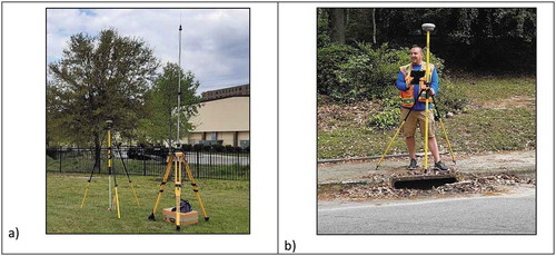
To obtain centimeter(s) level accuracies with short occupation times (e.g., 20 seconds or less) requires receiving and utilizing the observed errors from a base station in a real-time kinematic (RTK) approach. In the USA this base station location may be a National Geodetic Survey or state geodetic survey monument whose position has been established using other high-accuracy methods and integrated among local monuments in a network. Many states (e.g., North and South Carolina, Tennessee, Mississippi) and countries (e.g., Spain) have a network of continuously operating base stations, organized in a network, and real-time corrections are broadcast to users through a cellular network (Páez et al. 2017). Alternatively, a user might establish their own local monument using a static occupation (discussed previously) and subsequently occupy the monument with a dual-frequency GNSS receiver capable of deriving the errors and broadcasting the errors to a “roving” receiver (Figure 1). Alternative transmission methods have historically utilized packet radio but the emerging long-range radio (LoRa) may provide an inexpensive solution.

The expected accuracy of positions using the roving receiver degrades somewhat with increasing distance from the base station as the errors observed at the base station may be increasingly different from the rover’s environment (primarily the atmospheric attenuation). As a note, commercial vendors typically use base station positions very close (e.g., meters to a kilometer) to the rover receiver to generate and advertise accuracies; thus, the resulting accuracies would be expected to be very good. In a virtual reference network, such as a state real-time network, the appropriate corrections are created for a “virtual” position very near the roving procedure from a weighted average of nearby base stations. Thus, assuming the appropriate corrections vary across geographic space in a predictable manner the localized corrections in the virtual reference network somewhat simulate a close base station.

Finally, the types of positioning solution (i.e., DGPS, Float, FIX) in the RTK method are critical and have enormous impacts on realized accuracies – and are often misunderstood. A FIX² solution tracks the carrier wave of the satellite signal and resolves precision to approximately 1% of a single wavelength (~2-mm) by solving the integer ambiguities in the carrier wave. DGPS solutions are not a solution to a single wavelength and thus, considerably less accurate. For brevity, Float solutions will only be accurate to about 50-cm or worse while FIX solutions are commonly accurate to one or two centimeters. In short, for the highest accuracies the only solution that should be permitted for each observation used in the processing (single observation or averaging) is the FIX solutions. Not all GNSS processing software can screen for only FIX solutions.

Figure 1. GNSS survey grade receiver operating as a base station over a known position and broadcasting the errors at the position (a) to one or more roving GNSS receivers using a radio modem (b)

A common misperception of the accuracy of positions using a GNSS receiver is the assumption the observed accuracies are constant across landscapes. The common metric to estimate the quality of the geometric arrangement of available satellite signals at a position is called dilution of precision (DOP). Historically, the positional accuracies varied considerably in open horizon contexts simply because the availability of the GPS satellites were limited. With multi-constellation (i.e. GPS satellites plus the additional GLONASS, Galileo, and BeiDou satellites) receivers the problem of good geometric arrangements in locations without signal obstructions (e.g. buildings, heavy forests, topographically complex mountains, etc.) is virtually eliminated. Secondly, in compromised environments, the assumption that the RTK approach eliminates the blockage or multi-path of satellite signals from buildings, forests, etc. is false. The multi-path problem is also common in urbanized environments and under forest canopy. Multi-paths of satellite signals may also occur from topographic faces, particularly in non-vegetated landscapes where the user is close to the surfaces (a similar issue with proximity to buildings and metal fences). To emphasize, just because a FIX solution is observed on the display screen this does not imply the position is accurate to within a few centimeters and in fact, may be in error by meters or more resulting from multi-paths in a satellite signal.

3. Methodology

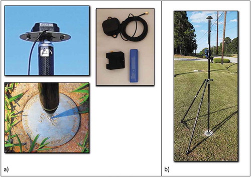
For this research, the Ardusimple2BLite kit, which includes the U-blox ANN-MB dual-frequency antenna, was evaluated as a typical low cost dual-frequency GNSS receiver (Figure 2(a)). The U-blox ZED-F9P chip is, after only one year, the most widely incorporated GNSS chip in many commercial GNSS receivers by – Emlid, Drotek, ArduSimple, etc. The Emlid kit is the most complete solution as it includes battery, Bluetooth chip, dual-frequency antenna, radio modem, and software. The Ardusimple SimpleRTK2BLite kit is the least expensive (~$300) kit but requires an external battery and user’s preference for software. Battery power is provided by any 5.0 V battery commonly used to recharge a cell phone. For this application, the SW Maps software was utilized (free software) which includes a built-in NTRIP client for receiving corrections via cellular from the South Carolina virtual reference network (SCRTN). The SW Maps app was set to only record FIX observations, either singly or through averaging. This latter restriction of only using FIX positions is not available in most apps but is critical for the highest accuracy. Without a FIX criterion, the resulting positional solutions may come from a mixture of Float and FIX positions (or worse, such as DGPS) and the user would be unaware. Prior to the initial testing, it was discovered the SimpleRTK2BLite GNSS receiver did not have the NMEA-HIGHPREC (i.e., utilizes centimeter-level computation in the receiver) setting enabled in firmware. With the default setting the derived heights are only precise to the decimeter. Enabling the high precision mode requires the use of either programming or through the U-blox U-Center Windows software suite (also free). After enabling high precision, the observations in the heights were reported as expected with centimeter precisions.

A Topcon fixed height (2.00-m) rover pole with calibrated bubble was used to hold the antenna. The U-blox antenna includes a built-in strong magnet and is intended to be attached to a metal plate. To mount and center the antenna on the fixed-height rover pole the antenna was first centered and mounted on a 10-cm ground plane with a 5/8” nut affixed to the bottom for attachment on the rover pole (Figure 2(b)). The precise X-Y-Z position of the observed location is actually the phase center inside the GNSS antenna. The phase center of the antenna is not the antenna reference point (ARP) but is typically offset above the ARP a centimeter or more (which impacts interpretation of the Z-values). For the U-blox ANN-MB antenna the phase center offset varies by less than 5-mm in all horizontal directions and less than 10-mm in the vertical. To be very specific, this phase center even varies somewhat with the angle of each satellite at a moment in time. For this research an average height offset of 7-mm above the ARP was assumed and used. In the research stage to replicate field collections, the combination of the antenna mount and phase center offset puts the observed position 1.7-cm above the top of the 2.0-m height rover pole; thus, all observations were 2.017-m above the ground.

The RTK receiver received RTCM corrections from the South Carolina Real Time Network (SCRTN) using a set of 45 continuously operating base stations. The SCRTN is a Trimble virtual reference network where the corrections (from GPS, GLONASS, and Galileo satellites) are weighted averages from the nearby base stations. The datum frame and coordinate systems for the SCRTN, all NGS monuments visited, and all occupied positions (latitude, longitude, and elliptical height) were in the NAD83 (2011) reference frame.

Figure 2. GNSS survey grade receiver (Ardusimple SimpleRTK2Blite) used for the empirical assessment and antenna (U-blox ANN-MB) mounted to ground plane with 5/8” nut on back for attachment to fixed height rover pole (a). The bipod and fixed height 2-m rover setup in b) is the same used for all 36 monuments

This research was meant to replicate the collection of ground reference data by remote sensing scientists and similar disciplines interested in “centimeter-level” observations. Positioning the 2.0-m fixed height rover pole over the target (e.g., aerial target) can easily introduce centimeters of error without the use of leveling. The errors caused by inaccurate positioning are greater in the X-Y domain and almost negligible in the Z-domain using a fixed-height pole. As is common in precision surveys a bipod with bubble-level was used to place the rover pole centered above the NGS monument (Figure 2(b)) which practically eliminates positioning errors. A “survey point” foot was used on the rover pole. The bipod (or tripod) is essential for occupations of many seconds and certainly minutes.

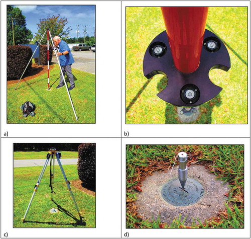
Two initial tests were conducted to evaluate 1) a possible antenna direction bias and 2) an appropriate averaging period for the occupation. With many geodetic antennas the phase center pattern results in a slight bias in one of the directions. This bias would be recorded and utilized if the antenna was calibrated and if the applications software used this calibration offset. The U-blox ANN-MB antenna has a north directional mark (i.e., the direction of the external wire). In the first initial test for antenna bias, observations were recorded with a fixed height tripod and attached 2.0-m pole (Figure 3(a)). The fixed height tripod includes three calibrated bubble levels and a 2.0-m height pole and is the same unit the SCGS uses to establish new monuments in South Carolina (Figure 3(b)). In the surveying community, a double-check on possible antenna offsets is often conducted by rotating the antenna 180-degrees between subsequent collections. An offset would be seen by consistent differences along a directed axis (i.e. the offset of the antenna from the antenna reference point). Fourteen average periods were conducted with 1-minute averages with the antenna pointed either north or south (seven each direction). The mean difference in observations with antenna pointed north versus south was only 0.137-cm. With the antenna pointed north the mean point was 0.137-cm to the east and a negligible difference in Y. Thus, the difference in the orientation of this antenna was considered negligible (i.e. the 1.3-mm was considered simply not significant).

The second test for averaging periods utilized the low height tripod, plumbed to the monument (Figure 3(c,d)), and back-to-back occupation sequences of 1) initialization of receiver, 2) averaged 20 seconds, 3) 5 minutes of 1-second fixes, 4) averaged 20 second occupation, 5) shut down receiver for 30 minutes, and repeat. Between each observation set, the receiver was reinitialized to provide some independence between observations. The initialization process involves downloading satellite almanac data, ephemeris data, time delays in the transmission from each satellite, and the current date/time of each satellite. Initial observations of 5-minute periods (300 single observations per period) every 30 minutes during a 6-hour afternoon were used to determine an appropriate occupation time to minimize typical variations in observations each second.

Figure 3. State geodetic survey director leveling fixed height survey pole with GNSS receiver antenna at monument EC2938 (a), three bubble levels on fixed tripod (b), lower tripod mount (c), and use of plumbed tripod for antenna (d)

Both tests were conducted at the NGS monument EC2938 located in the yard of the South Carolina Geodetic Survey office. This monument is commonly used by the surveying community for testing equipment to resolve problems. Of particular note in this study is one of the base stations in the SCRTN is on the same land parcel, 96 meters from the EC2938 monument. Thus, the RTK corrections (i.e. GPS, GLONASS, and Galileo) broadcast to the receiver on the South Carolina Real Time Network are primarily coming from an exceedingly close base station, effectively removing the additional error observed from longer baselines. The accuracies at this site would be expected to be very good and likely similar to the relative accuracies for RTK use where the user provided their own very close base station (emulating the common example from the GNSS marketing materials). The validation to be conducted after these two initial tests is more representative of the typical application in field research using base stations on a real-time network where the average distance to the nearest base station is much greater. In this study with the 36 NGS monuments, the average distance to the nearest base station was 16.2-km.

Scatter plots of the apparent movement (1-second observations) of a stationary GNSS antenna (Figure 4(a)) clearly indicate the variability in positions of about 2-cm during a 5-minute period. In this study the consecutive 1-second positions in a 5-minute period often resulted in a scatter clustered a centimeter or so away from the monument position, as in three of the 5-minute periods in the example (Figure 4(b)).

Figure 4. All observations (3700) in the 5-minute occupation periods during the 6-hour test (a). Four sequential 5-minute periods separated by 30-minutes in (b). Each second a new, non-averaged, FIX position was recorded. The reported SCGS monument where antenna was plumbed is shown as a green triangle with an expected accuracy of 0.21-cm (95% confidence level)

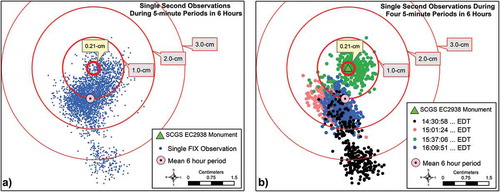
There appeared to be a possible ~1.0-cm bias caused by either monument error or maybe constellation similarities during the 6 hours. The NGS reported confidence for this monument was 0.21-cm (95% confidence level). Thus, the monument error was no more than 1/4^th of the observed bias at most. It is also possible the bias might result from the GPS + GLONASS + Galileo constellations observed in the 6-hour period. However, observations on the first test day (both a test in the afternoon and evening) also showed a similar bias.

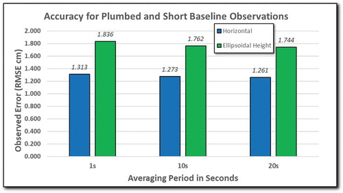
The accuracy of positions has long been known to improve with a greater number of observations over a longer averaging period, but at a decreasing rate of improvement with longer averaging times. The average change between the location of an observation each second was 0.31-cm. Subsequent observations are spatially correlated as typical with GNSS observations. Each 5-minute group of observations were clustered while notable differences were apparent between groups. By taking consecutive sets of observations at 10 and 20-seconds the average position and resulting error was computed. The average horizontal error (RMSE) of the 1-second, 10-second, and 20-second averages were 1.313-cm, 1.273-cm, 1.261-cm, respectively (Figure 5). The 10-second averages were significantly better than the 1-second observations (t-test; p = 0.0076). Similarly, the average error in the heights for the 10-second average (1.762-cm RMSE) was significantly better than the 1-second observations (1.836-cm RMSE). Thus, averaging at 10 seconds offered a notable improvement compared to 1-second observations. However, no statistically significant improvement was seen in either the horizontal or height errors between a 10-second and 20-second average. However, to be conservative a 20-second averaging period was chosen for the remainder of the study in replicating typically field applications. In summary, with such a short baseline to the nearest RTK base and for the effort in plumbing a perfectly leveled position the RMSEs are very low for such a low-cost receiver and antenna, even for the instantaneous observations.

Figure 5. Horizontal and height accuracies (RMSE) derived from grouping consecutive single observations in averaging periods from 1-sec, 10-sec, and 20-sec

The second part of the study used the same GNSS/antenna in a typical field study environment – where the proximity to the base stations is much greater (average of 16.2-km to the nearest), a fixed height 2-m rover pole for the antenna, and a bipod for leveling the antenna over the point of interest. Selection of NGS monuments for the research was based on quality of the monument and sky visibility at the monument site. Only monuments with an NGS modeled expected accuracy of less than 2.0-cm in both horizontal and vertical were selected. Using reference data with greater errors approaches the expected accuracy of the GNSS receiver under investigation. Finally, only monuments that were not under tree canopy were selected. Originally, all of the height modernization monuments were devoid of overhanging vegetated cover when established but some ten or twenty years of growth can create vegetated overhang (some completely shrouding the monument) that would not permit FIX positions to be obtained by the receiver. Also, it was desirable to select monuments in several counties as RTK performance may vary with distance from the nearest base stations participating in a correction solution. An initial set of 43 monuments were chosen in four counties (Richland, Lexington, Newberry, and Fairfield counties). Only monuments rated as “height modernization” (except for one notable cooperative station recommended by SCGS) were utilized as these locations exhibit the highest integrity in stability and modeled “truth” positions. The modeled accuracy of the monuments themselves were also collected from NGS, with an average 0.9-cm horizontal accuracy (95% confidence level) and 1.0-cm vertical accuracy (95% confidence level). Thus, these monuments were of higher accuracy as reference data than the anticipated GNSS-derived accuracies evaluated. Only monuments without surrounding trees that would obstruct satellite visibility were used. “Surrounding” trees means sites where the nearest trees were farther than 10 meters away. To be clear, most monuments were located where forest stands were now common nearby (greater than 10 meters) and thus, the nearby vegetation would have some impacts on the visibility of satellites on one or more horizons. No monument was located in perfect conditions (e.g., top of mountain or in an open field with no surrounding vegetation for hundreds of meters); thus, these reference data locations are very typical of open canopy research areas in suburban or rural, but not agricultural environments. Most sites were in the piedmont of South Carolina with gentle topography.

Each monument site was visited, and the monument “recovered,” as most monuments are often covered by landscaping or low vegetation growth. The monuments were visited once on six field campaigns between May 4 and May 24 of 2020. Each site visit involved locating the monument, leveling the antenna over the monument, initializing the receiver for 1-minute and initial RTK correction establishment through an NTRIP client, checking for a constant FIX position, and then recording a 20-second occupation. The initialization process (noted earlier) was performed before each temporal set of observations. By reinitializing between observation sets in this study some measure of independence is offered. Reinitializing the GNSS receiver is typically not necessary for a research project where multiple observations are taken at the same study site. In fact, observations (e.g. targets, validation points, etc.) are simply collected by moving from one location to the next and occupying each location of interest for a period of time (e.g., 20-seconds). However, in this research the drive between each subsequent site involved a 15 to 45-minute trip where the antenna (now inside the car) would not receive continuous satellite signals and, thus; the NTRIP connection and FIX solutions are lost.

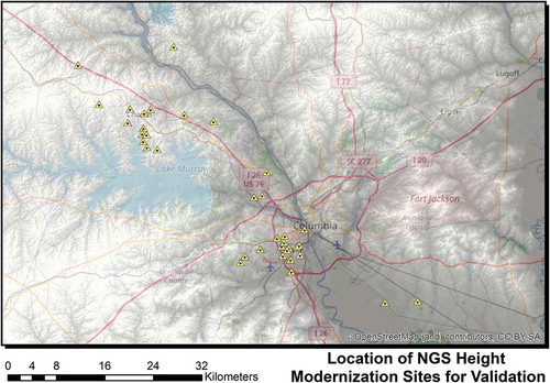
After visiting each of the 43 sites a total of 36 monument observations were included in the analysis (Figure 6). Monuments eliminated from consideration were because of surrounding trees (2), lack of cellular connections for NTRIP (3), automobile parked over the monument (1), and an overtopped fire ant mound (1).

Figure 6. Locations of the 36 NGS monuments recovered and where cellular and FIX observations could be observed

The analysis included descriptive statistics in the form of error frequency distributions, a test for normality in the error distributions, computation of signed mean errors (for a positive or negative bias), and RMSE (i.e., 68%) and Accuracy (i.e., 95%) statistics for the horizontal error and for vertical error, respectively. Following the well-known FGDC accuracy standards, the 95% error values were calculated from the RMSE statistics using the constants 1.7308 and 1.96 for the horizontal and vertical Accuracy statistics, respectively (FGDC 1998).

An estimate of the GNSS + antenna error with additional error from the reference source can be modeled with a simple error budget. Assuming the errors from the GNSS receiver are independent (i.e., uncorrelated) of any errors in the reported positions of the NGS monuments or other sources of error the error budget for the horizontal accuracy may be derived as (after Hodgson and Bresnahan 2004; Maling 1989):

$RMS{E^2}_{observed}=RMS{E^2}_{GNSS}+RMS{E^2}_{ref}+RMS{E^2}_{Usersetup}+RMS{E^2}_{phasecenteroffset}$

where,

RMSE_observed = error observed by comparing the receiver’s estimation to the reported position of the NGS monument,

RMSE_GNSS = actual error in the receiver’s estimation,

RMSE_ref = error in the reported position of the NGS monument,

RMSE_{User setup} = error from the user positioning the antenna/pole over monument,

RMSE_{phase center offset} = error from the antenna phase center and the reported position of the antenna.

The error in positioning and leveling a rover pole over the point of interest is unknown and tacitly assumed as negligible as there are no other empirical data to provide an estimate. (The author’s own experience from a calibrated level on a 2-m pole would be less than 0.5-cm.) The phase center error range for the ANN-MB receiver is known although a statistical estimate of the center error is unknown. Error from the phase center offset was regarded as negligible based on the initial test. Assuming these last two error contributions (RMSE_{User setup} and RMSE_{phase center offset}) are combined into the estimate for the reference error (now called RMSE_ref+) Equation (1)$RMS{E^2}_{observed}=RMS{E^2}_{GNSS}+RMS{E^2}_{ref}+RMS{E^2}_{Usersetup}+RMS{E^2}_{phasecenteroffset}$ can be rearranged as to derive the actual accuracy of just the GNSS receiver plus antenna:

$RMS{E}_{GNSS}=sqrt\left(RMS{E^2}_{observed}-RMS{E^2}_{ref+}\right)$

where,

RMSE_observed = accuracy of the GNSS observations using reference data,

RMSE_GNSS = intrinsic accuracy of the GNSS without additional reference data error,

RMSE_ref+ = accuracy of the reference data plus user pole setup and phase center error.

NGS provides estimates of each NGS monument’s positional error (as horizontal and vertical estimate). As noted earlier, for the set of 36 NGS monuments visited the average horizontal and vertical errors (RMSE_ref) are 0.9-cm (95% confidence level) and 1.0-cm (95%), respectively. Assuming the antenna and pole setup was negligible, the additional errors observed by a scientist with the GNSS use (RMSE_{ref+ =} RMSE_ref) was represented only by the NGS reported monument positional error.

4. Field test results

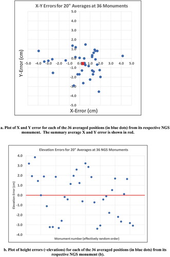
The distribution of errors in both the X and Y dimensions appear nearly centered around the monuments visited (Figure 7(a)). The mean signed error for X, Y, and Z were 0.285-cm, −0.550-cm, and −0.050-cm, respectively (Figures 7(a,b) and Table 1). The average X error is slightly positive and average Y error is slightly negative, suggesting an over prediction in longitude and under prediction in latitude. Using the t-test to see if the distribution of X errors were significantly different from 0.0 indicates no difference from a hypothesized population mean of 0.0 (p =.324705). However, there was a statistically significant difference in Y values (i.e., latitude) from a population mean of 0.0 (p = 0.012987). The statistically significant 0.5-cm southerly error suggests a similar bias in direction as noted earlier although considerably less (~1.0 cm in initial tests). Height errors are also not significantly different from a normal distribution and not statistically different from a population mean of 0.0 (p = .324044) (Figure 7(b)). The explanation for the horizontal southerly bias is not known. Discussions with the state geodetic surveyor director raised a few possible hypotheses (e.g., bias in NGS monuments from North American plate movement, real-time network bias) but none that could be appropriately tested.

Table 1. Summary Statistics from 36 Reference Points (in centimeters)

Statistic	X	Y	Horizontal (X and Y combined)	Height
Signed mean error	0.2854	−0.5459		−0.05
RMSEobserved (63% for horizontal or 68% for X, Y, or Z)	1.7146	1.3490	2.18	2.20
Accuracyobserved (95%)	3.3606	2.6445	3.77	4.31
Mean NGS expected monument accuracy (95%)			0.90	1.00
Intrinsic Accuracy of GNSS Receiver (after monument error removed)
RMSEGNSS (63% for radial or 68% for z)			2.12	2.13
Accuracy (95%)			3.67	4.18

The variation in errors is customarily expressed as RMSE for combined X-Y horizontal error (63% confidence) and vertical error (68% confidence), and Accuracy (95%) for both horizontal and height errors (Table 1). These observed RMSEs (2.18-cm and 2.20-cm) are quite surprising for an inexpensive dual-frequency GNSS receiver and antenna in field operations. The observed Accuracy statistics for the horizontal and height was 3.77-cm and 4.31-cm, respectively.

Figure 7. (a) Plot of X and Y error for each of the 36 averaged positions (in blue dots) from its respective NGS monument. The summary average X and Y error is shown in red. b. Plot of height errors (~elevations) for each of the 36 averaged positions (in blue dots) from its respective NGS monument (b)

Assuming the errors from the GNSS receiver are independent (i.e., uncorrelated) of any errors in the reported positions of the NGS monuments the error budget model for horizontal accuracy with these data is:

$RMS{E}_{GNSS}=sqrt\left({2.18}^2-{0.50}^2\right)=2.12$

Thus, as validated with the 36 NGS monuments the user’s real horizontal accuracy with this GNSS receiver and antenna would be 2.12-cm RMSE (or 3.7-cm at the 95% confidence level). Similarly, the accuracy for heights would be 2.13-cm RMSE (or 4.2-cm at the 95% confidence level). Historically, with only a single GPS constellation, an often-stated fact with GPS receivers was the vertical accuracy is less accurate than the horizontal accuracy, by 1.5 to 2.0 times. In this study using the laborious setup of a tripod and plumb bob when “perfectly” centering the antenna the difference between the horizontal and height accuracies was notable – 1.1-cm RMSE in horizontal and 1.76-cm RMSE in height. With the field visits to the 36 NGS monuments the horizontal and height accuracies were virtually the same. In typical field work the user is leveling a GNSS antenna over a point of interest where the antenna is affixed to the top of a 2-m high rover pole. Any slight leveling error can have a much greater effect on the horizontal centering of the antenna (thus, increasing the horizontal error) but has very little effect on the vertical height above the point of interest. Thus, the statement that the horizontal accuracies are much better than the vertical accuracies is not born out in practice for stop and go target surveys in natural resource data collections, except for laborious setup of instruments (e.g. a tripod and plumbing the antenna or a tribrach/laser).

As the reference data (i.e., NGS monuments) exhibited such low error in the piedmont sites the effects on the GNSS validation is almost insignificant. This is not always the case. In a typical application using GNSS for establishing aerial targets or collection of ground reference data (e.g. elevations) with high precision/accuracy sUAS imagery the reference data can have a more profound impact. For example, assume a sUAS derived DEM has a real accuracy of 2.0-cm RMSE (I use the acronym here to be RMSE_DEM). The scientist uses the same GNSS equipment and processing approach as in this study and collects validation data (with the same vertical accuracy as in this study of 2.1-cm RMSE_ref+). By using the error budget model equation (i.e., Equation (2))$RMS{E}_{GNSS}=sqrt\left(RMS{E^2}_{observed}-RMS{E^2}_{ref+}\right)$ we can apply the concept to error in a digital elevation model (DEM). Rather than experiencing a 2.0-cm accuracy the analyst would actually observe in his/her validation a DEM accuracy of 2.9-cm with GNSS-derived reference points as:

$RMS{E}_{observedinDEM}=sqrt\left(RMS{E^2}_{DEM}+RMS{E_{ref+}}^2\right)$

$RMS{E}_{observedinDEM}=sqrt\left({2.0}^2+{2.1}^2\right)=2.9$

The observed accuracy of the DEM of 2.9-cm is 45% greater than the actual accuracy of the DEM. As the reference data error approaches the accuracy of the data to be validated the reference error impacts increase. It should be obvious from Equations (1$RMS{E^2}_{observed}=RMS{E^2}_{GNSS}+RMS{E^2}_{ref}+RMS{E^2}_{Usersetup}+RMS{E^2}_{phasecenteroffset}$) and (2$RMS{E}_{GNSS}=sqrt\left(RMS{E^2}_{observed}-RMS{E^2}_{ref+}\right)$) the observed accuracy RMSE (e.g. RMSE_{observed in DEM}) can never be, theoretically, less than the accuracy of the reference data. Simply stated, if the accuracy of the GNSS receiver used in a validation (e.g., 2.1-cm RMSE) is greater than 0.0-cm the observed accuracy of the geospatial product will be greater than 0.0-cm even if the geospatial product actually has 0.0-cm error. Unfortunately, the accuracy of the reference data is seldom presented as an error budget model in geospatial studies while the observed accuracy is considered standard practice. This is unfortunate and as geospatial research continues in the centimeter-ish levels using GNSS receivers as reference data collectors the true accuracy of geospatial products will be clouded.

5. Mountainous & forested landscapes

5.1. Forested landscapes

It is desirable to also evaluate the performance of the low-cost receiver (or any GNSS receiver) in mountainous areas or forested areas, as two anonymous reviewers encouraged. Others have investigated the effects of forest canopy on recreational receivers (Rodríguez-Pérez, Álvarez, and Sanz-Ablanedo 2007), smartphone GNSS receivers (Tomaštík et al. 2017) and dual-frequency receivers operating in DGPS mode. Sigrist, Coppin, and Hermy (1999) tested DGPS receivers under forest canopies of different amounts and concluded the effects on both horizontal and vertical accuracy are exponentially related to canopy closure. There are several issues with conducting a performance evaluation of a real-time network receiver (RTK) in these two conditions. First, it is well-understood in the GNSS community the dual-frequency receivers cannot reliably solve for the integer ambiguities in evergreen forested environments and deciduous canopy (i.e. leaf-on conditions); thus, obtaining FIX solutions providing centimeter-ish resolutions are not reliable. The problem of multi-path in forested environments also further complicates the use of dual-frequency receivers in these conditions. Even if FIX solutions can be obtained the accuracy is unreliable without other checks.

Næsset and Gjevestad (2008) studied long occupation times (i.e., 15 minutes to 2 hours) in a forested environment using a dual-frequency and two constellation receiver (GPS and GLONASS) to collect phase data for precise point positioning (PPP), such as is commonly performed with subsequent use of OPUS. Their results indicate for observation periods of 15 minutes it was very difficult to even derive positional FIXes and with the longest occupation period of 2 hours positional accuracies ranged from 27-cm to 88-cm depending on the forest canopy coverage.

However, it is possible, but unreliable, to obtain FIX solutions with a network RTK receiver and with repeat visits (e.g., hours apart to allow for changing constellations) to the same point. Bakula, Oszczak, and P-Mieczkowska (2009) documents this problem in their study. A reliable solution can only be asserted if the same positional values are obtained in repeat visits under different satellite constellations. In previous research, the present author has been able to occasionally obtain repeatable FIX solutions enabling the establishment of a local base for subsequent use of a total station and back-sights. The strategy used is to first obtain a FIX lock on satellite signals outside the forest and then slowly move near, and sometimes within, the forest – a method called “carrying the lock.” Nonetheless, the unreliable nature of positions estimates and the requirement for repeat visits results in substantial levels-of-effort for many applications.

5.2. Mountainous landscapes

The challenge of using and particularly, validating, the performance of a GNSS network (e.g. RTN or RTK) receiver in a mountainous environment is from three problems: 1) occlusion of satellite signals from mountains, 2) occlusion of cellular signals supporting RTN from mountains, and 3) availability of high-quality reference data (e.g., NGS height modernization sites). The occlusion of satellite signals from mountainous landscapes (or even evergreen forests) results in a satellite geometry with a limited range of angles between tracked satellites. With any GNSS use (e.g. PPP, PPK, RTN, RTK, DGPS, or code-based) the ideal arrangement of satellite signals is where the angles between satellites used and the receiver is very large (e.g. near-horizon to near-horizon). Impacts on positional accuracies from occluded signals is greatest on the height estimates of a position.

In an attempt at providing some guidance on the performance of the GNSS receiver in mountainous environments a set of NGS height-modernization stations (20) located in the South Carolina mountains were identified. From this initial set of 20 height modernization stations a subset was created by modeling all stations that were located in a topographic environment where at least one of the cardinal horizons (north, south, east, west) above 20-degrees was occluded. Finally, using cellular coverage area maps (i.e. AT&T) a final set of 10 NGS height modernization sites with topographically induced occlusions and expected cellular coverage were visited (Figure 8). The NGS modeled expected accuracies of these 10 reference monument positions were, not surprisingly, poorer than the expected accuracies from the non-mountainous reference sites, but all below 1.5-cm horizontal and 1.8-cm height (95% confidence level).

Figure 8. Locations of 10 NGS height modernization sites in South Carolina mountains for validation. Thick black lines are county boundaries

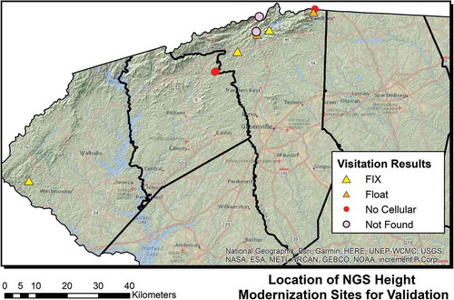
A visit to each of the 10 sites on two field campaigns on August 16 and 17 of 2020 (i.e. also full canopy conditions as with the 36 sites visited in the piedmont) resulted in only three sites in which a FIX solution could be realized and maintained for at least 20-seconds. And for these three sites a FIX solution could only be obtained by first collecting observations for a period of 5-minutes at one site, 10-minutes at another site, and 20-minutes for the third site. Three of the sites did not have cellular access despite advertised cell company coverage maps. Only a FLOAT solution could be obtained at two of the sites. The station monument could not be recovered at two sites (and possibly had been destroyed). The resulting horizontal and height errors for the three sites ranged from −0.4-cm to 3.8-cm and from −3.6-cm to 5.9-cm, respectively. The summary horizontal and height accuracies (RMSE_observed) of the three sites were 2.79-cm and 5.12-cm, respectively. The horizontal errors were somewhat higher (2.79-cm versus 2.18-cm) than the piedmont sites while the height errors were approximately twice as large (5.12-cm vs 2.20-cm). The reference data error was not removed from these three sites as the sample set was so small (i.e., 3) so the RMSE values should be compared to the RMSE_observed values in Table 1. The larger height errors were not surprising as the topographically induced occlusion of satellite signals minimizes the angular geometric configuration of viewable satellites. Because of the limited number (3) of observations these findings in mountainous terrain should be interpreted as guidance but not as a complete validation. However, the finding that FIX solutions could be found at three of the sites and float solutions at two of the sites is further evidence of the challenge in using survey grade receivers in mountainous landscapes. Further, the reliance on a cellular network for broadcast corrections in mountainous terrain is problematic. Like the satellite signals the cellular signals are also line-of-sight transmission and occluded by the mountains. The use of a satellite-based real time network delivery service (e.g. TrimbleRTX) can obviate the cellular-based delivery issue but not the availability of reference sites for a validation.

As a note, when the South Carolina Geodetic Survey (SCGS) works in the mountainous area of South Carolina there are times they do not rely on the real-time network (and dependency on cell service) but rather establish their own local base position with a receiver – the classical approach to RTK (pers. comm. Matt Wellslager). If a geodetic control monument, with a published coordinate cannot be found in the location of survey, the SCGS staff will set the base station receiver on a site suitable for Global Navigation Satellite Systems (GNSS) data collection, occupy the site from a minimum of 2 hours to preferably 4 hours and record the L1/L2 carrier phase data. This observed data set downloaded from the base station will be uploaded, via e-mail, to the NGS Online Positioning User Service (OPUS). A coordinate (latitude, longitude, and height) will be calculated using data from three “nearby” continuous operating reference stations (CORS) stations (a sparser distribution than the 45 base stations in the SCRTN real-time VRS network) and emailed back to the user. This coordinate will be used as the base position for correction observables. Instead of using real-time corrections from a cellular network the corrections are sent via radio modem from the base receiver to the rover receiver (up to 1.0 miles away line-of-sight).

Most state-level reference networks deliver correctional data over cellular networks. A rigorous test in mountainous terrain with a network receiver would not be possible relying on cellular networks for delivery of corrections. Alternatives would be from satellite-based correctional data or locally created base stations as most state geodetic survey offices conduct. However, these local base stations would likely not be as accurate as the NGS height modernization stations, thus, introducing error levels that may approach the typical accuracies of the GNSS receiver under testing. The limited set of reliable reference data and these issues in mountainous terrain render a rigorous validation nearly impossible.

6. Discussion

The issues noted for collection of RTK data with a high precision dual-frequency GNSS receiver are reiterated here. These issues should be stressed in academic courses and for others only familiar with the traditional code-based GNSS use. In most field applications the antenna will be mounted on a fixed height rover pole and ideally, use a bipod or tripod to maintain a leveled and centered position while measuring with the GNSS receiver. The latitude, longitude, and ellipsoidal heights (i.e. for deriving elevations) computed by the GNSS receiver are dependent on the user’s ability to position the GNSS antenna precisely over the desired location to be measured. Even the use of a rover pole requires the usual calibration of the bubble level to insure the positioning ability of a rover pole. There are a wide variety of dual-frequency antennas available and most of the inexpensive antennas are not calibrated and thus, there may be some error, albeit small, such as less than 1-cm, introduced in the observations. Fortunately, the availability of relatively inexpensive calibrated antennas is becoming greater and the average phase center offset can be compensated for.

The integration of low-cost GNSS receivers in a plug-and-play kit is evolving. The GNSS receiver kit used in this study contains the same U-blox dual-frequency multi-constellation receiver as in most other vendors’ low-cost receiver packages. These receivers are becoming widely used by the GIScience community with only vendor-supplied precision and accuracy estimates. Care must be taken in the choice of software and the default output from the GNSS receivers. For example, the HIGHPRECISION setting in the firmware of the U-blox receiver in the kit received was not initially enabled, resulting in decimeter precision of heights. The GNSS receiver was evaluated only as a roving receiver operating on the South Carolina real time network, receiving corrections from multiple nearby base stations as a virtual nearby base station. The SCRTN at present only supplies corrections for GPS, GLONASS, and Galileo – not BeiDou. Inclusion of the BeiDou corrections may also improve accuracies although this is not expected to be a dramatic help except for possibly the mountainous areas.

Most inexpensive or free GNSS software applications permit averaging although few restrict the averaged positions to only use FIX positions. If the goal is to reach accuracies approaching a centimeter(s) then only FIX positions should be used and averaged; thus, only apps supporting such restrictions should be utilized. There are other uses for these high precision GNSS receivers and antennae, such as with unmanned aircraft or applications involving a moving base as well as the moving rover. In these dynamic applications the positions are typically instantaneous (e.g. each second or up to 15 times per second) rather than averages. The error of such instantaneous single observations would be expected to be somewhat greater (particularly with a moving aircraft/receiver) than from the 20-second averages found in this research. Future research studies should investigate the accuracy in moving receivers (although the problem of reference data is elusive).

The results from this study indicate for typical applications in non-mountainous environments a very low-cost dual frequency and multi-constellation GNSS receiver and antenna can reliably obtain positional accuracies in the horizontal plane and heights of approximately 2.1-cm (RMSE_GNSS) with only a 20-second average of observations. These results are nearly identical to the Topcon GRS-1 dual frequency multi-constellation receiver with calibrated PG-A1 antenna the author has used for almost ten years. Such accuracies are often needed for establishing reference targets and check points in sUAS mapping and terrain modeling applications. Remote sensing scientists with a similar GNSS receiver and occupations could use these reported values as estimated accuracies of the ground control points for parameter estimates in SfM photogrammetry applications rather than the default values. Scientists and practitioners monitoring landscapes could use these results in establishing confidence values in the change in positions, such as in erosion/deposition, sediment budgets, etc. (James et al. 2012). Having an empirical estimate of the positional accuracy provided through a GNSS receiver also permits the use of an error budget model in separating reference data error from the total observed error in the validation process. When higher accuracies are needed (e.g., 1.3-cm horizontal and 1.7-cm height RMSEs) it is possible if the user exerts additional effort in plumbing positions and using very short baselines, although this effort is atypical in most fieldwork.

Acknowledgements

The author would like to express his appreciation for Matt Wellslager, Director of the South Carolina State Geodetic (SCGS) Director and Lewis Lapine, former SCGS Director and Director of the National Geodetic Survey, for their comments and guidance on GNSS issues and the SCRTN throughout the last ten years.

Data availability

The data that support the findings of this study are available from the corresponding author, upon reasonable request.

Disclosure statement

No potential conflict of interest was reported by the author.

Notes

1. There are many frequencies and the naming conventions by the four global constellations varies. For example, the GPS satellites use L1, L2, L2C, and L5. The availability of frequencies changes with new generations of the satellites. The important point here is two different frequencies are essential to measure the atmospheric attenuation in the ionosphere and thus, remove this error source.

2. The often used terminology is a FIX solution solves for the integer ambiguities while the DGPS and Float solutions do not.

References

- Bakula, M., S. Oszczak, and R. P-Mieczkowska. 2009. “Performance of RTK Positioning in Forest Conditions: Case Study.” Journal of Surveying Engineering 135 (3): 125–130. doi:10.1061/(ASCE)0733-9453(2009)135:3(125).
- El Shouny, A. E., and Y. Miky. 2019. “Accuracy Assessment of Relative and Precise Point Positioning Online GPS Processing Services.” Journal of Geomatics 13 (3): 215–227. doi:10.1515/jag-2018-0046.
- Federal Geographic Data Committee (FGDC). 1998. “Geospatial Positioning Accuracy Standards Part 3: National Standard for Spatial Data Accuracy.” FGDC-STD-007.3-1998.
- Hardin, P. J., F. Lulla, R. R. Jnsen, and J. R. Jensen. 2019. “Small Unmanned Aerial Systems (Suas) for Environmental Remote Sensing: Challenges and Opportunities Revisited.” GIScience & Remote Sensing 56 (2): 309–322. doi:10.1080/15481603.2018.1510088.
- Hodgson, M. E., and P. Bresnahan. 2004. “Accuracy of Airborne Lidar-Derived Elevation: Empirical Assessment and Error Budget.” Photogrammetric Engineering & Remote Sensing 70 (3): 331–339. doi:10.14358/PERS.70.3.331.
- Jackson, J., R. Saborio, S. A. Ghazanfar, D. Gebre-Egziabher, and B. Davis. 2018. “Evaluation of Low-Cost, Centimeter-Level Accuracy OEM GNSS Receivers.” Report No. MN/RC 2018-10. http://www.dot.state.mn.us/research/reports/2018/201810.pdf.
- James, L. A., M. E. Hodgson, S. Ghoshal, and M. M. Latiolais. 2012. “Geomorphic Change Detection Using Historic Maps and DEM Differencing: The Temporal Dimension of Geospatial Analysis.” Geomorphology 137 (1): 181–198. doi:10.1016/j.geomorph.2010.10.039.
- Maling, D. H. 1989. Measurements from Maps, 577. New York, N.Y.: Pergamon Press.
- Næsset, N., and J. G. Gjevestad. 2008. “Performance of GPS Precise Point Positioning under Conifer Forest Canopies.” Photogrametric Engineering and Remote Sensing 74 (5): 661–668. doi:10.14358/PERS.74.5.661.
- Nie, Z., F. Liu, and Y. Gao. 2020. “Real-time Precise Point Positioning with a Low-cost Dual Frequency GNSS Device.” GPS Solutions 24 (9). doi:10.1007/s10291-019-0922-3.
- Páez, R., C. Torrecillas, I. Barbero, and M. Berrocoso. 2017. “Regional Positioning Services as Economic and Construction Activity Indicators: The Case Study of Andalusian Positioning Network (Southern Spain).” Geocarto International 32 (1): 44–58. doi:10.1080/10106049.2015.1120358.
- Rodríguez-Pérez, J. R., M. F. Álvarez, and E. Sanz-Ablanedo. 2007. “Assessment of Low-Cost GPS Receiver Accuracy and Precision in Forest Environments.” Journal of Surveying Engineering 133 (4): 159–167. doi:10.1061/(ASCE)0733-9453(2007)133:4(159).
- Sigrist, P., P. Coppin, and M. Hermy. 1999. “Impact of Forest Canopy on Quality and Accuracy of GPS Measurements.” International Journal of Remote Sensing 20 (18): 3595–3610. doi:10.1080/014311699211228.
- Tomaštík, J., Jr., J. Julián Tomaštík Sr, Š. Saloň, and R. Piroh. 2017. “Horizontal Accuracy and Applicability of Smartphone GNSS Positioning in Forests.” Forestry 90: 187–198. doi:10.1093/forestry/cpw031.
- Unger, D. R., D. L. Kulhavy, and I.-K. Hung. 2013. “Validating the Geometric Accuracy of High Spatial Resolution Multispectral Satellite Data.” GIScience & Remote Sensing 50 (3): 271–280. doi:10.1080/15481603.2013.805585.
- Williams, R. D., M. Lamy, G. Maniatis, and E. Stott. 2020. “Three-dimensional Reconstruction of Fluvial Surface Sedimentology and Topography Using Personal Mobile Laser Scanning.” Earth Surface Processes and Landforms 45: 251–261. doi:10.1002/esp.4747.