Analyzing short term spatial and temporal dynamics of water presence at a basin-scale in Mexico using SAR data

ABSTRACT

The dynamic nature of continental water body covers is a main indicator of the status of this ecological capital and its trends on the land surface. With synthetic aperture radar (SAR), various water coverage processes can be identified using satellite data. This study proposes the use of a basin-level analysis with SAR images at a medium spatial resolution to perform a regional spatial-temporal analysis for detecting water presence. It develops a methodology to improve the separation of water bodies from other land covers by using a texture analysis, a support-vector machine classification, and the gray level co-occurrence matrix (GLCM). GLCM-mean texture parameter was found to offer sufficient texture information for separating the water class from the land class by providing a more homogeneous measurement of water bodies. The case under study is the Grijalva River Basin, Mexico, a region that requires more in-depth research so that the management of surface water coverage can be integrated with ecosystems, particularly those that are subject to intense human activity. The entire basin was mapped using a series of observations from Sentinel-1. This study produced a total of 36 water body maps with an acceptable classification accuracy of over 90% for each year studied (2016, 2017, and 2018). Water presence was also quantified, resulting in a set of maps containing regional detail, from which temporal data can be obtained on areas with water presence year-round and areas with seasonal flooding. Frequency maps with a 10-km unit cell as the spatial unit were used to detect trends and thereby identify water distribution patterns. The results show the importance of ongoing, basin-level quantifications of zones with dynamic water presence and those with stable water presence.

KEYWORDS:

• Grijalva Basin
• Sentinel-1
• seasonal characterization
• texture information

1. Introduction

The dynamics of the water cycle are associated with the biological cycle of various ecosystems (Gleeson et al. 2020). Since the permanence of freshwater bodies is subject to threats and pressure from land-use changes, information is needed about changes in river flow during dry seasons, as well as changes in flood zones during periods of flooding and the degree of eventual ecological recovery from precipitation.

The spatial and temporal dynamics of water body surfaces reflect their sensitivity to environmental fluctuations and human impact (Hogeboom 2020). Lakes and rivers are dynamic environments that change over different time scales. Precipitation and drought are two factors that affect their levels. Other factors are runoff, slope angles, and the influence of tides on river mouths.

Given the new technological developments and innovations in obtaining observational data of the land from space, different types of sensors (active and passive) can now be used to generate cartographic products that represent water presence and the morphological caracteristics of water bodies at different scales (global, national, regional, and local). To make advances in the use of multi-temporal Optical Landsat data series (TM, ETM+, and OLI sensors) with 30- and 90-m spatial resolutions, Yamazaki, Trigg, and Ikeshima (2015) proposed conducting inter-annual monitoring based on the analysis of historical data from the Landsat data family. This study obtained the G3WBM-Global 3 arc-second Water Body Map product (90-m resolution), whose latest update is the G1WMB- Global 1 arc-second Water Body Map (30-m resolution). The Global Surface Water Explorer (GSWE) platform, developed by the European Commission Joint Research Centre (JRC) based on 32 years of observation, provides the following products for monitoring the occurrence and dynamics of surface water: Surface Water Occurrence, Surface Water Occurrence Change Intensity, Surface Water Recurrence, Surface Water Seasonality, and Transitions in Surface Water Class (Pekel et al. 2016). Advances in scale have been made with the ESA-CCI Land Cover S2 Prototype LC Map of Mesoamerica (Defourny et al. 2018), which was developed to assess the capabilities of Sentinel-2 data. This map has a 10-m spatial resolution and 10 different land cover classes, including water bodies.

Cloud cover and day/night conditions have not been found to affect the ability to use Synthetic Aperture Radar (SAR) to produce water body inventories. The international initiative by the CCI Land Cover project to generate a global map of open permanent water bodies includes a series of products at a medium resolution of 150 m (CCI WB-Map v3.0 (Santoro et al. 2015) and CCI WB-Map v4.0 (Lamarche et al. 2017)). This initiative demonstrates the ability to use time-series data from historical images from Envisat Advanced Synthetic Aperture (ASAR) for the years 2005–2012. Odermatt et al. (2018) presented a study that delineates lakes at the global level using ENVISAT data (2002–2012).

The water body products in these previous studies are representative of the observation period and the spatial scale at which they were generated. They present methodological differences related with which type of sensors and image processing techniques were used, as well as the multi-temporal typological systems used to classify water bodies. The accuracy of global maps has not always satisfied the detail that users require for local-scale applications.

Various factors at the local level need to be more thoroughly investigated in order to obtain basin-level baseline data on the spatial distribution of freshwater at finer scales, as well as to obtain information about its status and historical seasonal trends based on SAR data.

This study contributes to the advances in medium-resolution monitoring by developing the methodological capability to map the seasonal presence of water. It examines the benefits and limitations of basin-level, multi-temporal data with a high frequency of observations of water bodies, by using open data from the Sentinel-1 (S1) data series, which are sensitive enough to detect water body surfaces and can be used to monitor fluctuations. Generating maps at the basin level is important because of the need to identify rapid, seasonal changes in the water surface and to capture the dynamics of seasonal flooding, which is a growing problem in regions with large amounts of precipitation. S1 is helpful for generating time-series data.

Although S1 data provide a high temporal resolution, regular intervals need to be used. The study herein is based on a monthly time series, which makes it possible to measure seasonal water surfaces, determine the extension of water presence, and analyze trends. A shorter time interval improves the identification of flash floods.

This study focused on the Grijalva River Basin as a case study. It analyzed a short time period of 3 years to explain the temporal variability of the surface water bodies in the basin. In order to assess water status for this case study, 36 monthly water body maps were produced at the basin level, which delineate and delimit the width of the rivers and lakes. This work was based on the system characteristics of the S1 time-series, with vertical-vertical (VV) polarization, as the main source of images for the period 2016, 2017, and 2018.

The methodology for the image processing was based on the use of a texture parameter with the gray level co-occurrence matrix (GLCM) to enhance the recognition of the water surface pattern in the SAR image. Texture provides information about the spatial distribution of differences in backscattering coefficients between neighboring pixels in the SAR image. This work extends the idea presented by Hall-Beyer (2017) by proposing that the GLCM-mean texture parameter be used as a descriptor of “internal texture.” When studying the delineation of water bodies, this parameter provides a less noisy, more homogenous measurement of the spatial distribution of water/no water covers, which helps the task of segmentation. Studies that have reported on the use of texture parameters to improve the extraction of water bodies have been primarily conducted with Radarsat 1 and 2 (Yeong-Sun, Hong-Gyoo, and Choung-Hwan 2007; Bolanos et al. 2016; Li and Wang 2015), or with Sentinel-1 for images of individual, medium water bodies (Valdiviezo-Navarro et al. 2019). According to those authors, monitoring water bodies by incorporating different texture parameters with data from SAR images increases the accuracy of water/no water masks in high mountainous regions. Nevertheless, it is difficult to compare the usefulness and effectiveness of the texture parameters that were selected because of the different conditions that were processed, and because GLCM has rarely been used to estimate open surface water for large areas at the basin level. As a consequence, it can be concluded that the texture approach can be applied to much larger areas in order to obtain a detailed regional map using S1 data. To address the limitations mentioned above and to understand the contribution of texture, the use of the GLCM-mean texture parameter is proposed, which provides valuable quantitative information with which to differentiate water and no water areas at low, medium, and high elevations.

Support vector machines (SVM) have been found to perform well for segmenting SAR images (Haykin 2009). Some authors (Wentao-Lv and Wenxian-Yu 2010; Pôssa and Maillard 2018) who have mapped water surfaces using an SVM classification with SAR data have obtained good results. For these reasons, the study herein used SVM for the segmentation of images.

When comparing the previous methods with the method proposed herein, the following aspects of how the present study delineates water bodies stand out: i) SAR C-band characteristics are used, which are not limited in their ability to provide information for a regional multi-temporal study on a monthly basis or a shorter interval, whereas optical methods present time gaps that affect the final information on trends and changes in water presence. ii) The dynamics of surface water bodies of different forms and sizes are characterized using time-series maps of water presence, rather than static maps representing a snapshot of a water body at a specific point in time. iii) To more accurately estimate surface water, machine learning is improved with the use of SVM along with texture information and topographic measurements. iv) The GLCM-mean parameter is used to provide a less noisy, more homegenous measurement of the spatial distribution of water/no water covers, which helps the task of segmentation using SVM. v) The estimation of the surface water cover that is present throughout the entire Grijalva River Basin is developed and characterized using S1 data with an interval of roughly 1 month, in order to monitor the temporal variability of the basin’s hydrology for water bodies ranging in size from 50 to 50,500 ha.

The present study is structured as follows. First, the study area is described. Then, the methodological proposal for digital image processing is developed. The results of the water bodies are then presented using monthly water presence maps. To observe multi-temporal trends, additional layers are also shown, including annual seasonal water frequency and frequencies based on rainfall-runoff behavior in the Grijalva River Basin. Lastly, the method for using texture, the significant findings related to water presence in the upper and lower elevations of the Grijalva River Basin, and the benefits and limitations of this study are discussed.

2. Materials

2.1. Study area

The Grijalva River Basin is located in the states of Tabasco and Chiapas, Mexico. It measures 5,218,407 ha (CONAGUA 2019) and spans lower and upper elevations. The basin is located in a humid tropical region with constant cloud cover. Given the geographic location, weather, and topography of this region, it presents several challenges. The vegetation is highly diverse in both the upper and lower elevations. The aquatic ecosystems consist of lagoons as well as rivers and their tributaries, which distribute freshwater to wetlands, lakes, and mangroves, and for agricultural, livestock, and fishing activities. Various ecosystem-water-food-energy functions interact. And extreme flooding continually occurs in the basin (Palomeque de la Cruz et al. 2017).

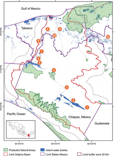
The main river in this region is the Grijalva River, one of the mightiest in Mexico, which has a large fluvial network of dams, lagoons, channels, drainages, streams, and rivers. This river runs through or alongside several urban and rural localities. The dynamics of the river has historically been controlled with control infrastructure in response to significant natural changes, and its morphology has been greatly altered. Figure 1 shows the important sites along the Grijalva River.

Figure 1. Study area. The boundaries of the Grijalva Basin, with water bodies and protected nature reserves. The boundary shown includes a 20-km buffer. 1) Grijalva River channel pattern (the area of the basin represents the Mexican portion only), 2) Angostura Dam, 3) Grijalva River, 4) Chicoasen Dam, 5) Malpaso Dam, 6) Grijalva River, 7) Peñitas Dam, 8) Mezcalapa River, 9) Samaria River, 10) Carrizal River, 11) Villahermosa City – Grijalva River to Gulf of Mexico, and 12) Usumacinta River

2.2. Description of data

2.2.1. Data

2.2.1.1. *S1 data

Image selection considered the fact that processing SAR data entails solving problems that are caused by the effects of i) geometric distortion (layover, foreshortening, and shadows projected by mountainous areas); ii) radar signal interactions with surface structures, wind (which increases the roughness of the surface), the presence of aquatic vegetation (which modifies the radar’s return signal and generates unusual tones in the image), moisture gradients on lake shores (which produce classification problems), and the presence of sediments (which lead to over-segmentation problems); and iii) radiometric distortion (influence of topography on backscatter).

In just one image, the S1 sensor can cover a swath width of 250 km, with a moderate spatial resolution of 22.5 m (slant-range) x 20 m (azimuth). This design provides sufficient data for observing natural changes in water bodies. SRTM (Shuttle Radar Topography Mission) is a digital elevation model (DEM) with a spatial resolution of 30 m, which was used for the geolocation of the images.

A total of 181 S1 C-band images were obtained from Level-1 Ground Range Detected (GRD) S1 SAR, downloaded from the Copernicus Open Access Hub (https://scihub.copernicus.eu/dhus/#/home). For Mexico, VV polarization data were available for the year 2016, and both VV and VH polarizations were available for 2017 and 2018. Studies have shown that VV polarization (vertical transmit, vertical receive SAR backscattering coefficient, ${\sigma }_{\mathrm{V}\mathrm{V}}^0$) is useful for differentiating water/no-water areas (Pôssa et al. 2018; Mahdianpari et al. 2020). This work used VV polarization for all three study years. The characteristics of this polarization are suitable for both open water bodies and temporarily flooded vegetation (Tsyganskaya, Martinis, and Marzahn 2019).

In order to cover the study area, 5 observations per month were required, consisting of 3 observations from Track 99 and 2 from Track 172. The three images from Track 99 were used as the main basis for generating the mosaic for each month. They were from the same date and covered the majority of the Grijalva River. When generating the mosaic, 2 scenes were selected from Track 172, with the same date as the Track 99 images. Table 1 presents the list of images used. Given the availability of online data, 3 images from Track 34 and 1 from Track 136 were also used, in addition to the images from Tracks 99 and 172.

Table 1. Observation dates of the Sentinel-1 images

	Day of year (DOY)
Monthly Mosaic	1	2	3	4	5	6	7	8	9	10	11	12
Track-99-2016	23	47	71	119	143	167	191	239	263	287	311	359
Track-172-2016	04	52	76	100	148	– -	196	244	268	292	316	364
Track-34-2016						150
Track-99-2017	–	53	65	113	125	161	197	221	245	281	329	353
Track-172-2017	–	58	70	118	130	166	202	226	250	286	322	346
Track-34/Track-136-2017	1,8
Track-99-2018	25	48	84	120	144	168	192	222	270	294	342	360
Track-172-2018	29	53	89	113	149	173	187	221	263	299	347	365

2.1.2. Images for obtaining reference data

The images were selected for the process of obtaining reference data. It is feasible to use high-resolution data as reference data (Olofsson et al. 2014). To validate the reference data, historical images were selected from Google Earth, SPOT-6, and Sentinel-2. The data used were obtained from SPOT-6 (CNES) telemetries from the Agro-Foods and Fisheries Information System (SIAP in Spanish), under the “AIRBUS DS” license. Resolutions ranged from 5 to 2.5 m. Free data from Sentinel-2 were used, at a resolution of 10 m.

Images were obtained from the Copernicus Open Hub, and the Sentinel data were viewed and processed with SNAP (Sentinel Application Platform) software. Table 2 presents the images that were selected, the selection criteria, and the images to be validated. This table includes the date of the binary layer that was validated, the date of the reference image, and difference in days (with the criterion mentioned previously of a maximum of 3 days).

Table 2. Reference images and characteristics of the data to be validated (lower elevation = LE, middle elevation = ME, upper elevation = UE)

Monthly Mosaic Number (ID) Year-month	Date of binary layer	Location	Date of reference image	Source of reference image	Difference in days
2016–04	28	LE	28	Google Earth	0
2016–05	22	LE	24	Google Earth	2
2016–11	30	LE-ME	29	Google Earth	1
2017–05	05	LE	08	Sentinel 2	3
2017–10	08	LE-ME	08	SPOT-6	0
2017–12	19	LE	19	SPOT-6	0
2018–01	24	LE	24	Sentinel 2	0
2018–02	17	LE	16	Google Earth	1
2018–07	23	UE	23	Google Earth	0

2.1.3. Auxiliary data

•Mexican Continuous Elevation Cartography (CEM 3.0). This digital elevation model (DEM) dataset is from the National Institute for Statistics and Geography (INEGI -México 2015). CEM 3.0 has a 15-m cell size. Color digital orthophotos of Mexico were used, at a scale of 1:20 000 and a resolution of 1 m. These data served as a reference for obtaining ground control points (GCP).

3. Approach and methodology

The flow diagram shown in Figure 2 describes the SAR image processing sequence for differentiating water bodies from other types of land covers. The following sections describe SAR pre-processing, GLCM processing, classification, post-processing, validation, and the spatial analysis of water dynamics.

Figure 2. Sentinel-1 data processing for extracting water bodies and spatial analysis methods

3.1. Remote sensing data processing

3.1.1. Pre-processing

The S1 images were processed using standard SAR processing techniques, including updating orbit metadata with accurate orbit information and removing thermal noise. The calibration of this process resulted in the conversion of digital level values into backscattering coefficient values based on satellite metadata obtained from ESA. For GRD products, the equation $value\left(i\right)=\frac{{\left|D{N}_i\right|}^2}{A_i^2}$ was applied, where $value\left(i\right)$ corresponds to the backscattering coefficient, DN is the digital pixel values, and A_i is one of sigma nought (i). The values σ⁰ were converted to dB based on the formula ${\sigma }_{\mathrm{d}\mathrm{B}}^0=10.\mathrm{l}\mathrm{o}{\mathrm{g}}_{10}{\sigma }^0$. Spatial averaging (multi-look) was then used to reduce speckle noise. In the spatial domain, the radar images presented a degree of noise known as “speckle,” and based on filter testing, the decision was made to use the refined Lee Sigma filter, as proposed by Pôssa and Maillard (2018). The last stage of the pre-processing involved terrain-geocoding using a DEM, in this case SRTM (30 m). This step had two objectives. One was to improve the quality of the SAR product by decreasing the main geometric distortions caused by the effects of radar image formation. The other was to orient the image with respect to the geographic terrain model, a procedure known as geometric terrain correction (GTC). The geocoding was calculated with the precision of satellite orbit data and metadata to ensure that the geographic location was satisfactory. The resampling method was nearest neighbor. During this processing, a mask was applied that included only continental water areas. The geographic coordinate system World Geodetic System 84 (WGS84) was used for the cartographic projection.

The selection of ascending or descending orbit was based on a visual evaluation and the calculation of root mean squared error (RMSE). The tests found that in ascending orbit, the length of some of the pixels shifted in zones with nearly vertical slopes. Furthermore, in a region located in the general study area that contains a system of medium and small water bodies, López-Caloca, Escalante-Ramírez, and Henao (2020) found that descending orbit had fewer geometric distortions than ascending orbit. The planimetric precision of the resulting SAR image in descending orbit was evaluated when reconstructing the image’s geometry. Images captured in March 2018 by Track-99 were selected based on this procedure. Two regions representing different topographies were taken from two S1 radar images: a low-relief zone measuring 4068 meters and a high-relief zone measuring 4121 meters. PCI Geomatics software was used to evaluate the RMSE by generating automatic GCPs based on the orthophoto from INEGI as a reference image.

3.1.2. Classification of Sentinel-1 data to obtain water/no water binary maps

In order to prepare the data for classification, a texture analysis was applied to the pre-processed images in accordance with parameters proposed by Haralick, Shanmugam, and Dinstein (1973), based on the statistical analysis of the intrinsic properties of surface textures and a set of statistical descriptors of the spatial dependence of the gray-level values in the image. GLCM describes the frequency with which a combination of two pixels in an image is produced (gray level values) within a predefined calculation window. It takes into account the relation between two adjacent pixels: the reference and the neighboring pixel. Input parameters include orientation, shift, gray level input values, and the size of the window or kernel. GLCM involves generating several texture parameters: contrast, dissimilarity, homogeneity, angular second moment, maximum probability, entropy, mean, correlation, and variance.

The Haralick model was calculated based on parameters from the SNAP tool by the European Space Agency, with a window size defining the spatial relation between 5 × 5 neighbors (to prevent loss of details). The spatial relation with each neighbor was in four directions: 0°, 45°, 90°, 135°. The quantizer value was based on a probabilistic approach.

The quantization level was represented by a range over 128 bins. This ensures greater detail in the texture variables calculated. GLCM features are defined as the probability of 2 pixels with the same value being separated in an image by distance d. This probability can be found by counting the number of times that the value of the reference pixel and that of its neighbors is separated by distance d. The shift or distance designated between a pair of pixels was 4. In addition, high computational demand was required for texture extraction from a complete scene.

To select the best texture parameter, the coefficient of variation (CV) was calculated for each Haralick feature, which is defined as:

(1) $CV=\frac{\sigma }{\mu }$(1)

where σ is the standard deviation and µ is the samples obtained in 5 × 5 subwindows. RStudio free software was used to calculate and analyze the correlations of the texture parameters.

The SVM algorithm was characterized by defining a hyperplane for the separation of classes, which was constructed and adjusted with training data from the water/no water classes. The training pixels were representative of each class so that the classification process would adequately separate the pixels in the image. The data were processed using the classifier from the Monteverdi toolbox, by the French space agency. The present study used a linear kernel, which did not require defining parameters.

The result eliminated isolated pixels, closed and filled interior water body areas that were omitted in the classification, and reassigned areas that were obviously incorrectly classified, such as airports. The final products obtained as a result of all these procedures were 36 mosaics, one for each month of each year (2016, 2017, and 2018), containing only the locations showing water cover information. These products were used to perform the validation process.

For the spatial analysis, raster data from the binary water/no water mask were converted to vector format, considering 8-connected neighbors.

3.1.3. Post-processing

The results of the digital image processing step were quantified by generating a “study area mask” in post-processing. The generation of this mask took into account the low- and high-relief subdivision of the basin, which was obtained by calculating the degrees of slope in the study area based on terrain shape information from CEM 3.0. The slope percentage was generated with ArcGIS 10.2.2 using its spatial analysis tool. This was then reclassified into two ranges: a low-relief zone with equal or less than 5° and a high-relief zone with more than 5°. This threshold was defined by considering slope gradients under 5°. Other adjustment parameters (geomorphological features, mountain chains, the river runoff system) were determined based on the map of slopes, with its subdivision of the basin into low- and high-relief zones.

The “study area mask” also served to eliminate misclassified areas from the “water bodies mask,” which eliminated false pixels that were confused with water bodies due to final noise and shadows from mountains, particularly in the high-relief zone. This method was applied in accordance with other studies. For example, Cao et al. (2019) eliminated slope values that exceeded 15° using an SRTM DEM. Santoro and Wegmüller (2014) proposed using a terrain slope value with a threshold of 10°, which can be modified according to the type of slope (slight, moderate, or steep) for the use of SAR data at the global level.

3.2. Validation

The validation process involved a statistical assessment and a comparison with other products. The statistical assessment was based on Olofsson et al. (2014) and Pontius and Santacruz (2014). The following steps were used to perform the validation: calculation of the sample size; random assignment of sample sizes for the categories resulting from the classification of radar images (water/no water); selection of reference images from Google Earth, SPOT-6, and Sentinel-2; visual interpretation; obtainment of the water/no-water category from reference images of randomly assigned sampling points, based on the calculation of the sample size by category; obtainment of the confusion matrix for area; and calculation of overall accuracy (or agreement) and omission and commission errors.

According to the procedure established by Olofsson et al. (2014), the sample size should be calculated using a stratified random sampling to estimate accuracy or overall agreement. Olofsson et al. (2014) suggested calculating with the expression proposed by Cochran (1977):

(2) $\eta \approx {\left(\frac{\mathrm{\Sigma }{W}_i{\mathrm{S}}_i}{\mathrm{S}(\widehat{O)}}\right)}^2$(2)

where ƞ is the number of monthly units, S($\hat{O}$) is the standard error of the estimated overall accuracy desired (for example, values of 0.01), W_i is the mapped percentage area of class i, S_i is the standard deviation of stratum i and is calculated as follows:

(3) $S_i=\sqrt{U_i\left(1-U_i\right)},$(3)

where U_i is the user’s accuracy for class i. Olofsson et al. (2014) established that relatively stable classes (that present less errors of commission) can have S_i values near 0.9, and classes with more variations (which therefore have higher errors of commission values) can have S_i values between 0.6 and 0.7. The authors indicated that experiences from previous classifications are useful for determining S_i values.

The first criterion for selecting the images for obtaining reference data (see Table 1) was to choose those with dates near the dates of the radar images. As indicated (see Table 2), 3 days was the maximum permitted difference in dates. Data were taken from cloud-free areas in accordance with the criterion of minimum cloud cover for the images to be validated, and manageable cloud cover (maximum of roughly 20%) for the reference image. The reference area included the Grijalva River Basin with a 20-km buffer zone around the basin.

Given the availability of reference data images, only three radar images from each year could be validated. Of a total of 9 images selected, 5 had no difference in days, 2 had a difference of 1 day, 1 had a difference of 2 days, and 1 a difference of 3 days. Five of the reference images selected were from Google Earth, 2 were from SPOT-6 data, and 2 were from Sentinel-2. Track 99–1 was the one that coincided with 8 of the 9 reference images. In terms of time period, the images included months from the beginning, middle, and end of the year, giving this validation exercise good representativeness.

3.3. Information generated to study water dynamics

For the analysis of water presence, the following water/no water maps were used to produce thematic maps, with definitions based on temporal criteria and the characteristics of the water cover:

i)Frequency of Water Presence (FWP). These water presence maps were generated with S1 data. They provide information on the detection of water and the annual behavior of water surfaces. Monthly observations are grouped on an annual time scale, with a maximum water presence value of 12 months and a minimum of 1 month. The study years include 2016, 2017, and 2018. FWP is calculated with the following formula:

(4) $\mathrm{F}\mathrm{W}\mathrm{P}=\frac{{\sum }_{i=1}^{N}w}{N_{obs}}X100$(4)

where N_obs indicates the number of observations for each year and w is the binary mask, where w = 1 indicates water and w = 0 indicates land, per pixel.

The study herein considered water bodies to be permanent when FWP >75% and seasonal when 25%<FWP≤75%, in accordance with Deng et al. (2019). These two types of water presence were calculated based on $\mathrm{F}\mathrm{W}\mathrm{P}$ data.

ii) Water Presence Dynamic per 10-km Cell Unit. This product assesses the spatial distribution of water presence, and is based on the calculation of the percentage of inland water per grid cell, with a 10-km resolution.

A cell size of 100 km² was defined based on recommendations from monitoring models by the Dartmouth Flood Observatory, generated by Kundzewicz, Pińskwar, and Brakenridge (2012). The amount of water in each cell was calculated with a two-layer zonal statistics algorithm, which included: a file defining the surface water in each cell, in shape format, and monthly binarized water/no water vector maps. These maps were grouped according to seasonality, defined by the rainfall-runoff behavior in the Grijalva River Basin over a 15-year period, as proposed by Arreguín-Cortés et al. (2014). As a result, four groups were defined: frequency of water presence during the dry season (FWP-DS) (March and April); frequency of water presence during the rainy season with tropical influence (FWP-RSTI) (May, June, July, and August); frequency of water presence during the rainy season with autumn-winter influence (FWP-RSAWI) (September, October, and November); and frequency of water presence during the rainy season with winter influence (FWP-RSWI) (December, January and February). Each grouping of months was calculated inter-annually. For example, the frequency of water presence during the dry season represents the behavior of this season (March and April) over the 3 years.

4. Results

4.1. Geometrical accuracy

The following results were found when evaluating the images from day-of-year (DOY) 84 in descending orbit with GTC. For the low-relief zone, an RMSE of 4.8 m was obtained for the X component and 6.2 m for the Y component, with a 95% confidence level. For the high-relief zone, an RMSE of 7.6 m was found for the X component and 6.5 m for the Y component. The adjustment was better with the image of regions with slopes under 5°, which is consistent with the fact that geometric distortions are strongly related with topography, specifically, SAR data are very precise in low-relief zones. The zone with slopes over 5° is clearly seen to have been corrected by pre-processing, which is consistent with pre-processing’s aim to correct errors that occur during image acquisition due to the sensor and the terrain. Note that geometric distortion is reduced when using a good DEM spatial resolution.

4.2. Texture results

Table 3 shows the results of the coefficient of variation. The data from the refined Lee Sigma filter are presented in the column without texture. The other columns show each texture parameter after applying speckle filtering: contrast, dissimilarity, homogeneity, angular second moment, energy, entropy, GLCM-mean, and GLCM-variance. The GLCM texture image does not provide specific statistical information on the separability of water. Texture was calculated for complete scenes. Three scenes from Track 99 were analyzed: one from the lower elevation, one from the middle, and one from the upper elevation. DOY 71 was selected for 2016, DOY 75 for 2017, and DOY 84 for 2018. The lowest CV values are shown in bold.

Table 3. Coefficient of variation results for lower (LE), middle (ME), and upper elevations (UE) for the following textures: contrast (CON), dissimilarity (DISS), homogeneity (HOMO), angular second moment (ASM), energy (ENE), entropy (ENT), GLCM-mean, and GLCM-variance

ID	WITHOUT TEXTURE	CON	DISS	HOMO	ASM	ENE	ENT	GLCM- Mean	GLCM- Variance
2016-LE	0.1311	0.3516	0.1960	0.2103	0.1016	0.0788	1.0609	0.0766	0.1518
2016-ME-UE	0.1989	0.2407	0.1368	0.1223	0.1883	0.0939	0.1028	0.0852	0.1544
2016-UE	0.1744	0.3610	0.2069	0.1563	0.2645	0.1303	0.1117	0.0971	0.1960
2017-LE	0.1148	0.3087	0.1715	0.2801	0.1237	0.0585	0.1388	0.0582	0.1166
2017-ME-UE	0.2044	0.4280	0.2511	0.1668	0.3371	0.1666	0.2340	0.1116	0.2254
2017-UE	0.1209	0.2502	0.1387	0.1315	0.1480	0.0725	0.3276	0.0701	0.1495
2018-LE	0.4844	0.5794	0.3268	0.2783	0.3819	0.1865	0.1991	0.1367	0.2768
2018-ME-UE	0.2061	0.4981	0.2786	0.3913	0.2039	0.1958	0.1090	0.1053	0.2176
2018-UE	0.1214	0.2789	0.1580	0.1748	0.1412	0.0958	0.1808	0.0615	0.1274

To quantify the degree to which a linear relation exists among Haralick texture features, bimodal distributions were analyzed and compared based on two water/no water systems. Figure 3 presents the histograms for each of the 8 texture parameters. The image at the bottom represents the size of the image used for the upper and lower elevations. What is verified here is a strong relation among the graphs of the histograms shown in this figure. The first line presents GLCM-mean, GLCM-variance, contrast, and dissimilarity, and the second line shows homogeneity, ASM, energy, and entropy. As can be seen, the bimodal form that represents water/no water is very notable for GLCM-mean, GLCM-variance, contrast, and dissimilarity. ASM and energy have positive asymmetric distributions and entropy has a negative asymmetric distribution.

Based on the images in Figure 3, Pearson (r) and Spearman ($S\rho$) correlations were calculated (95% confidence interval, $\rho <0.02$) for the 8 textures, by pairs, for the upper and lower elevations, where r was used for normal distributions and $S\rho$ for non-normal distributions. Since the distributions were bimodal and asymmetric, Spearman’s correlation was the final test used. The pairs of texture parameters with correlations over 0.99 were GLCM-mean/GLCM-variance, contrast/dissimilarity, and ASM/energy. Energy/entropy and dissimilarity/homogeneity were inversely correlated. This coincides with the images of the upper and lower elevations. Table 4 provides more detailed findings from the Spearman correlation.

Figure 3. Histograms represented by bar frequencies, for the upper and lower elevations of the basin, in decibels (DB)

Table 4. Results of the texture correlation tests performed with the Spearman test (Sp.) for the following textures: contrast (CON), dissimilarity (DISS), homogeneity (HOMO), angular second moment (ASM), energy (ENE), entropy (ENT), GLCM-mean, and GLCM-variance (lower elevation = LE, upper elevation = UE)

TEXTURE PARAMETER	CON	DISS	HOMO	ASM	ENE	ENT	GLCM-mean	GLCM-variance
CON-LE CON-UE	1 1	0.9925 0.9961	−0.8894 –0.8233	−0.8426 –0.6781	−0.8426 –0.6782	0.8695 0.6781	0.7012 0.7571	0.7389 0.7968
DISS-LE DISS-UE		1 1	−0.9303 –0.8572	−0.8824 –0.6985	−0.8824 –0.6986	0.9052 0.6985	0.7165 0.7558	0.7527 0.7945
HOMO-LE HOMO-UE			1 1	0.9561 0.8177	0.9561 0.8177	−0.9606 –0.8188	−0.7135 –0.6416	−0.7397 –0.6668
ASM-LE ASM–UE				1 1	0.9991 0.9999	−0.9932 –0.9984	−0.6949 –0.5748	−0.7182 –0.5917
ENE-LE ENE-UE					1 1	−0.9932 –0.9984	−0.6950 –0.5748	−0.7182 –0.5917
ENT-LE ENT-UE						1 1	0.7045 0.5739	0.7296 0.5909
GLCM-mean-LE GLCM-mean-UE							1 1	0.9974 0.9965
GLCM-variance-LE GLCM-variance-UE								1 1

4.3. Accuracy assessment classification

Overall accuracy was assessed at the basin level. Table 5 presents the results from validating the 36 water/no water binary layers obtained when processing the radar images, which was based on the 3 months selected from each year. The validation included: total number of pixels per category for each binary layer, total ƞ and the assignment to each category, corrected points and errors per category, and the value of the parameters of agreement (omission, agreement (A), and commission). Accuracy values were obtained in accordance with Pontius and Santacruz (2014).

Table 5. Validation results for the images selected for the three study years (accuracy = A, overall agreement = OA)

Monthly Mosaic Number ID	Number of Pixels		ɳ (Points)		Correct		Errors		Land			Water			Overall
	Land	Water	Land	Water	Land	Water	Land	Water	Omission	A	Commission	Omission	A	Commission	Omission	OA	Commission
2016_04	1,311,916	229,770	103	103	94	102	9	1	0	78	7	7	15	0	7	93	7
2016_05	7,468,237	469,132	120	98	107	96	13	2	0	84	10	10	6	0	10	90	10
2016_11	1,420,840	29,414	111	111	107	107	4	4	0	94	4	4	2	0	4	96	4
2017_05	105,014,444	7,359,734	109	109	107	87	2	22	1	92	2	2	5	1	3	97	3
2017_10	32,958,133	657,267	112	112	108	109	4	3	0	95	4	4	2	0	4	96	4
2017_12	12,678,411	1,024,322	110	106	103	105	3	5	0	90	3	3	7	0	3	97	3
2018_01	2,909,575	4,959,080	57	97	54	96	3	1	1	35	2	2	62	1	3	97	3
2018_06	23,634,108	1,680,008	109	109	107	108	2	1	0	92	0	2	7	0	2	98	2
2018_07	2,804,909	102,893	111	111	111	111	0	0	0	96	0	0	4	0	0	100	0

^aValues of omission, A, and commission shown as percent of domain, as suggested by Pontius and Millones (2011).

As can be seen, total ƞ (water) fluctuated, with values ranging from 97 to 112. To determine the sample size for May, the minimum $S\widehat{\left(O\right)}$ value of the water category was obtained, with equal assignment (the same number of ƞ_i for both categories). As can be seen by the omission value, 10 points belonging to the water class were assigned to the no water category, while 10 points that actually belonged to the no water class were assigned to the water category. These errors are acceptable, with an A of 90%. Therefore, the binary mosaic water/no water maps were found to be valid.

4.4. Short-term variability of water bodies

Figure 4 shows annual water frequency grouped by >75% and 25–75%, with close-ups of the different portions of the Grijalva River Basin for each year. Red represents low percentages indicating seasonal flood zones with the pooling of water or some type of flooding pattern. Blue represents permanent water presence, where no significant changes in water presence were found during the study period, that is, water was present during all 3 years.

Figure 4. Results from the annual and tri-annual water presence maps based on monthly time series. A close-up of different areas are shown for each year

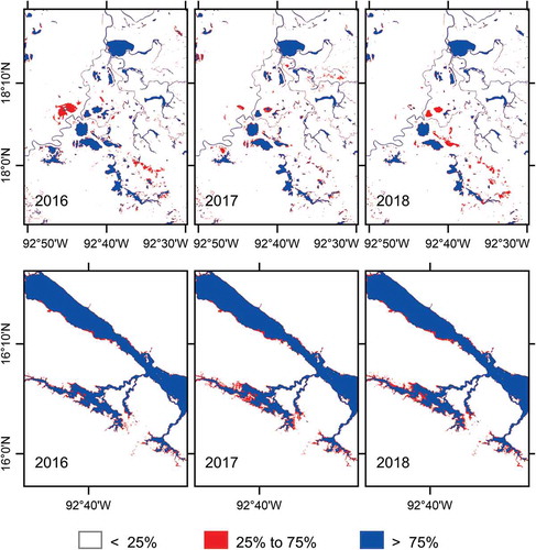
This analysis indicates the frequency of the number of months that had water present in each pixel. That is, the product for each year provides information about the monthly behavior of the water surface. Based on this analysis, the water bodies were separated according to water presence, where pixels that presented an FWP ˃75% were defined as permanent water presence, and those with an FWP between 25 and 75% were defined as seasonal, such as flood zones or areas with high moisture. For the entire Grijalva River Basin, permanent water bodies covered 102,403 ha in 2016, 98,303 in 2017, and 98,757 in 2018, and water bodies in the 25–75% range covered 22,087, 23,024, and 23,227 ha in 2016, 2017, and 2018, respectively. Water coverage was similar in 2017 and 2018, and slightly greater in 2016. The 25–75% range reflects dynamic water zones representing flood zones. The results show that these areas did not change drastically over the three study years.

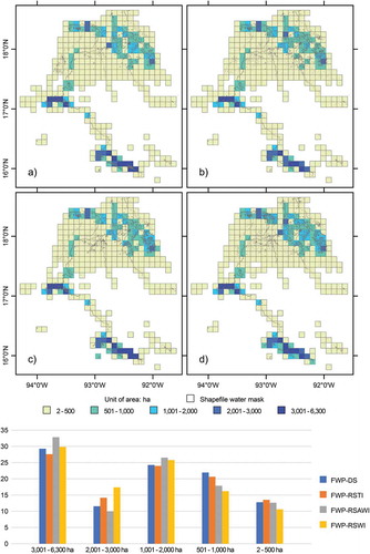
The presence of water cover over the entire 3-year time series was analyzed using monthly maps of the area per cell, which were grouped based on rainfall-runoff behavior for the four periods mentioned in Section 3.3. Figure 5 shows the distribution of water presence for the four groupings, along with the water distribution in the different geographic regions. The geographic space shown includes a 20-km buffer around the Girjalva River Basin. The area of water distributed per cell explains the variability in water for each cell. Blue indicates zones where more water is present, and light blue to yellow colors correspond to zones that have different degrees of water present. The figure shows the frequency of water presence during: FWP-DS (5a), FWP-RSTI (5b), FWP-RSAWI (5 c), and FWP-RSWI (5d). Over the course of this short-term study, maximum seasonal water bodies were present during FWP-RSWI, which was the period with the most rainfall, and particularly with the most runoff. More floods would be expected during this period. Very similar seasonal water bodies appeared during FWP-RSTI and FWP-RSAWI.

Figure 5(e) shows a bar graph of the distribution of the percentage of water presence for each grouping, per cell grid, obtained from area data. Water presence ranged from 27 to 33.55% for the 3000–6300-ha range, 10 to 17.4% for 2001–3000 ha, 23 to 26.8% for 1001–2000 ha, 16.2 to 20.8% for 501–1001 ha, and 10.63 to 13.56% for the 2–500-ha range. In general, differences among the groups ranged from 2.9 to 7.4%, which is attributable to changes in the areas of stable and dynamic water presence. Many seasonal changes in the edges of water bodies were found, which were due to their expansion during rainy seasons and their contraction during dry seasons. Dynamic changes also occurred in zones with extraordinary flooding (which normally contained a different type of land cover).

Figure 5. Maps of water percentage per 100-km² cell unit, in ha, grouped by seasonality over the entire 3-year time series: a) FWP-DS, b) FWP-RSTI, c) FWP-RSAWI, d) FWP-RSWI, and e) percentage of area (ha) for each grouping

5. Discussion

5.1. Methodology

The DEM used by this work corrected the geometric distortions in the radar signal produced by the sensor and the terrain during image acquisition, thereby reducing the effects of foreshortening, layover and radar shadows. In terms of GTC, the comparison of the behavior of RMSE with high-resolution images found good results for geolocation with the S1 SAR images in descending orbit with VV polarization. With respect to the DEM resolution, finer resolutions provided better adjustments of the SAR image in zones with steeper slopes, in terms of removing terrain distortions and decreasing the shadow effect. When reconstructing information in zones with water bodies located in complex topographies, tests of the data from sensors in ascending and descending orbits found shifts of 3 to 5 pixels in length in ascending orbit for the zone with nearly vertical slopes. Using these data for data fusion is not recommended unless orthorectification is performed with a digital elevation model that has better spatial resolution.

Some aspects to be considered when pre-processing SAR data are incidence angle normalization and radiometric calibration. Intensity data are converted to sigma-nought backscattering coefficients based on the incidence angle, which is calculated with the ellipsoidal model. In this case, the backscattering coefficient, σ°, varies according to the incidence angle. An incidence angle range prevents drastic changes in the incidence angle of the sensor’s geometry. Various authors consider an incidence angle between 30° and 50° to be adequate for delineating water bodies. In this case, it is important that the range be over 30° in order to obtain high contrast between land and water (Solbø and Solheim 2004; Wu et al. 2019). With angles over 50°, images tend to generate more radar shadows for water bodies located in mountainous regions. The shadow effect is also greater with high-resolution SAR images (Manavalan 2018). For this work, the incidence angle for all the data that were collected ranged from 29.1° to 46.0°. In the upper elevation, the DEM used by this study corrected the shadow effect throughout most of the length of the Grijalva River. This effect was found only in some of the small segments, and was identified and delineated with auxiliary cartography within the “study area mask.” Nevertheless, the resulting water maps need to be refined to decrease the effect of radar shadows very close to water bodies, and to obtain more details of water bodies (for example, narrow rivers) in upper elevations.

To improve the above results, a study of angular-based radiometric slope correction with the gamma nought value (ɣ°) is proposed, as described by Small, Miranda, and Meier (2009), or as Vollrath, Mullissa, and Reiche (2020) proposed for Sentinel-1 data. The purpose of this would be to compensate for variations in the incidence angle, which would improve the separability of radar shadows from water and provide greater classification accuracy when conducting future research.

The CV obtained for each texture parameter indicate a degree of despeckling. The lowest value was obtained with the GLCM-mean parameter, followed by the energy parameter. In both of these cases, the image with texture had a lower CV than the image without texture, for both the upper and lower elevations. A lower CV indicates relative constant σ ° values for the water bodies, since the calculation of CV is determined within surfaces, such as water bodies. For GLCM-variance, no significant differences in despeckling were found between the image with texture and the one without texture. As for the other texture parameters, contrast, dissimilarity, homogeneity, ASM, and entropy had a higher CV for the image without texture. The results from these tests indicate that GLCM-mean is the most suitable texture variable, since backscattering values for water bodies with a smooth surface are highly homogenous, while backscattering values are generally greater for terrain, as seen by the good separability of the bimodal distribution in the histogram. GLCM-mean is suitable for both upper and lower elevations.

Therefore, this study finds that the separation between water/land boundaries is adequate. The application of a dynamic range of 120 bins and a window size of 5 × 5 to calculate GLCM-mean enables differentiating water bodies from other types of land cover. The analysis of classified images suggests that the texture characteristics provided by GLCM-mean are among the best for classifying water bodies based on SAR data. Different texture window sizes can be evaluated to improve the connectivity and sharpness of water bodies such as rivers.

As expected, the correlation and histogram analyses indicate that several texture parameters were highly correlated. Some texture parameters also had images with more bit depth, showing good potential for improving image segmentation by combining spectral properties and texture data to separate various types of classes, including water/no water/ice (Park et al. 2020) and water/no water/vegetation (Cazals et al. 2016). Nevertheless, their use and application need to be evaluated and improved to prevent misclassification from not removing subtractive interference pixels. Several texture parameters should be used for the classification so that the information is not redundant.

The present study also indicates that the performance of the speckle filter method is limited, and it depends on the complexity of the terrain. Pixels with very low backscattering values remained because they were not removed or reduced by the speckle noise filtering process. This was seen as a prevalence of groups of pixels or small points (Wang et al. 2019) with low backscattering values in both lower and upper elevations, which were confused with the σ° response to water bodies, resulting in misclassified areas. With GLCM-mean, a moving window on an image was used to estimate local statistics at the level of the central pixel, with low-pass filters as the spatial filtering principle. The low CV value for GLCM-mean in both lower and upper elevations indicates a reduction in speckle, which is often mistakenly classified as water. This study also identified other benefits of using GLCM-mean, including a certain degree of flattening of the radar image and fewer misclassified areas.

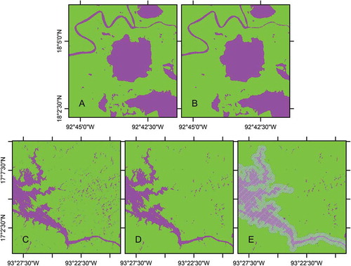
The “study area mask” that was designed for this basin represents the majority of water stored in the low-relief zone, and the boundaries of large water bodies (dams and the main river connecting them) in the mountainous regions are very visible. A pair of neighboring lagoon systems can be seen with little water cover due to the spatial configuration of the slope of the terrain. Nevertheless, for other basins that have a larger distribution of water bodies in mountainous areas, a specific mask needs to be defined in order to remove the specific locations that have layover and shadow effects from the DEM data (Vollrath, Mullissa, and Reiche (2020). Figure 6 shows the 2018-DOY 65 image of the lower (A-B) and upper elevations (C-D) before and after applying texture. Here, the VV backscattering image obtained with and without texture is seen. In Figure 6(e), the extraction of water (dark purple pixels) indicates extracted water masks. As seen in this example, the use of GLCM-mean improved the SVM classification in both upper and lower elevations. By including the GLCM-mean texture parameter, the final classification is cleaner and conserves water/land boundaries.

Figure 6. Water/no water binary mask. Lower elevation a) without texture, b) with texture. Upper elevation c) without texture, d) with texture; and e) with texture and mask of the study area

Data acquisition accuracy for the extension of water bodies was found to be high for the 36 monthly binary water/no water body mosaics analyzed. This water body product detected permanent and seasonal water bodies that were present over the three-year study period. Nevertheless, a larger number of monthly observations could help to monitor rapid changes in surface area during short-term flooding.

The classified texture images identified both the presence of water and seasonal changes in the extension of surface water bodies for a wide range of natural and artificial lakes with different sizes, from >50 ha (for example, Laguna Bosque Azul, Chiapas) to 50,500 ha (for example, Malpaso Dam reservoir, Chiapas). The principal rivers were also identified and delineated, including the Grijalva, Mezcalapa, and Carrizal rivers. As can be seen visually, several narrow rivers were not monitored due to the presence of vegetation and the loss of continuity in the rivers.

5.2. Benefits and limitations of the products obtained

As the results show, the Grijalva River Basin is a system of highly dynamic rivers and lakes requiring special and innovative monitoring approaches, such as continuous observations on a large regional scale. Complex river-lake interactions can be studied by observing the dynamic behavior of the rivers and lakes in this study area to better understand the implications for the ecological safety of the water in the water bodies, including current erosion on the edges of these water bodies.

By significantly reducing the time and financial costs required to assess the condition of water resources, the methodology described herein contributes to the study of the Grijalva River Basin and the management of lakes and rivers at a large basin scale.

In the 36 mosaics of information on water body coverage generated with SAR, the presence of discontinuous zones can be seen all along the Grijalva River due to the effect of increased infrastructure such as highways, dams, and a large number of bridges. A deep and narrow canyon known as Sumidero Canyon is located between the Chicoasen and Malpaso dams. The SAR maps of the upper elevation did not show information on the topographical area of this canyon because of its 1,000-m high walls. The lack of SAR information is most evident in the upper elevation, as well as in areas with complex topographies where the radar signal is not reflected back to the sensor.

During months with high precipitation, low elevations can contain moist zones, complex wetland systems, and pooling of water that could be identified as open water bodies, thereby creating problems with delineating water bodies. Therefore, these areas need to be studied with in situ validation. In order to prevent these problems, this study only included a water presence over 25%.

Radar also identifies interior vegetation throughout a river, whether floating on the fluvial system or remaining on its banks. When aquatic vegetation covers the width of the river, the processed image shows a discontinuity in the river. The delimitation of vegetation is determined by the natural conditions of a river, including its seasonality and variations in flow. As explained by Mendoza-Carranza et al. (2010), the identification of discontinuities due to riverbank vegetation serves as a parameter for assessing the ecological status of rivers, and according to Mattey-Trigueros et al. (2017) it also has an ecological function. For example, the present study found that water barely flows in the Old Mezcalapa River, or does not flow at all for months. Sentinel-1 SAR did not detect this river since there was little water and a good deal of surface vegetation.

Given the limitations in the SAR backscattering response to water bodies during periods when vegetation is present, a mask with the identification of these areas can be included. For these areas, incorporating information from cloud-free optical images such as Sentinel-2, with the same date, is recommended for areas with problems involving floating/seasonal emerging vegetation. Given that the detection of water bodies decreases with the VV band during the rainy season, when precipitation is high and windy conditions are present, the VH (vertical transmit, horizontal receive) band is recommended for those cases since it is less sensitive to those conditions.

This study was based on a binary classification (water/no water). For future studies, a thematic classification with more classes would make it possible to analyze additional classes, such as those found within water bodies (floating and submerged vegetation) and surrounding them at the landscape level, among others.

The image processing described herein provides promising results for the production of consistent surface water products. This approach requires more research in upper elevations to decrease the effect of geometric distortions and to apply angle incidence normalization, using a free-data DEM with a higher global or national spatial resolution.

Tools provided by the ESA’s Copernicus project can be used to explore automation with the proposed steps, including texture and the threshold method. Those tools enable implementing new ways to process images for chain processes that automate work flows for information extraction with the SNAPPY (open code) interface, which reduces computing time.

6. Conclusions

This study assessed the value of Sentinel-1 data for describing the spatial and temporal variability of water bodies. Findings show that Sentinel-1 images can be used to collect multi-temporal information on water presence in Mexico’s Grijalva River Basin. It was possible to adequately separate water/no water classes using both a SVM classifier and GLCM-mean texture datan. The study herein worked with SAR images of regions located in lower and upper elevations. The binary water mask made it possible to define the boundaries of water bodies and to adequately identify water presence. The statistical validation indicates that the results are reliable. This methodology to detect water presence by using the semi-automated procedure described herein can be applied to other basins, as well as to monitoring on the national level.

A frequency analysis was used to obtain detailed water maps at a local scale, which helped to detect highly dynamic water bodies and to evaluate water presence in the region. General maps at a regional scale were also used in order to better understand the overall situation with the extension of water presence.

An inventory of surface water presence was created for a time window of 3 years, and the results confirm the presence of zones with permanent water bodies and flood zones. This is a key component for managing water resources and for understanding their variability in space, in order to meet the needs of the residents in the region. These products contribute to diagnosing changes in the coverage of water bodies and to better understanding the freshwater dynamics in the Grijalva River Basin.

This work also generated information at the basin level that can be useful for other geographic and climatic regions with characteristics similar to the study area. And it produced global maps based on SAR data to meet the challenge of detecting water when there is a large variety of water conditions on different terrains.

Author Contributions

Investigation: AALC, FOTS, FL; Conceptualization, AALC.; Methodology, AALC.; Coefficient Variation, AALC; Correlation Analysis FL,AALC; Validation, FOTS, AR. and PH.; Image Processing: ALC, PH, AR, Formal Analysis, ALC; Cartographic: AALC,PH,FL; Analysis Spatial: FL, AALC, Writing – Original Draft Preparation, AALC.; Review Version AALC, FOTS.; Visualization, FL; Vector data, GR.

Acknowledgements

The authors thank the three anonymous reviewers for their constructive comments durings the review process. We also would like to thank the project coordinators, E. Martínez and J. Chapela for their support. The authors also thank the GeoINT-CentroGeo, particularly A. Morales and M. Ledesma for the data pre-processing service, and R. García-García for supporting the image design for this document.

Disclosure statement

No potential conflict of interest was reported by the authors.

Additional information

Funding

This work was funded by National Mexican Science Council (CONACYT) with the Project granted to CentroGeo, FORDECYT 2018-10. Award: 297259;Consejo Nacional de Ciencia y Tecnología [297259].

References

- Arreguín-Cortés, F. I., H. Rubio-Gutiérrez, R. Domínguez-Mora, and F. D. Luna-Cruz. 2014. “Análisis de las inundaciones en la planicie tabasqueña en el periodo 1995-2010.” Tecnología y Ciencias del Agua 5 (3): 05–32. On-line 2007-2422.
- Bolanos, S., D. Stiff, B. Brisco, and A. Pietroniro. 2016. “Operational Surface Water Detection and Monitoring Using Radarsat 2.” Remote Sensing 8 (4): 285. doi:10.3390/rs8040285.
- Cao, H., H. Zhang, C. Wang, and B. Zang. 2019. “Operational Flood Detection Using Sentinel-1SAR Data over Large Areas.” Water 11 (4): 786. doi:10.3390/w11040786.
- Cazals, C., S. Rapinel, P.-L. Frison, A. Bonis, G. Mercier, C. Mallet, S. Corgne, and J.-P. Rudant. 2016. “Mapping and Characterization of Hydrological Dynamics in a Coastal Marsh Using High Temporal Resolution Sentinel-1A Images.” Remote Sensing 8 (7): 570. doi:10.3390/rs8070570.
- Cochran, W. G. 1977. “Stratified Random Samplig.” In Sampling Techniques. 3rd ed. 127–130, New York: Wiley.
- CONAGUA. 2019. “Disponibilidad de cuencas hidrológicas.” México: Comisión Nacional del agua. http://sina.conagua.gob.mx/sina/tema.php?tema=cuencas&n=nacional
- Defourny, P., O. Arino, G. Kirches, C. Brockmann, M. Boettcher, C. Lamarche, B. François, J. Transon, and F. Ramonio. 2018. “In Technical Document: ESA CCI-LC Algorithm Theorical Basis Document.” ESACCI-LC-Ph2_CCN2_ATBD_v.06. On-line. https://2018mexicolandcover10m.esa.int/documents/ESACCI_CCN2_ATBDv0.6.pdf
- Deng, Y., W. Jiang, Z. Tang, Z. Ling, and Z. Wu. 2019. “Long-Term Changes of Open-Surface Water Bodies in the Yangtze River Basin Based on the Google Earth Engine Cloud Platform.” Remote Sensing 11 (19): 2213. doi:10.3390/rs11192213.
- Gleeson, T., L. Wang-Erlandsson, S. C. Zipper, M. Porkka, F. Jaramillo, D. Gerten, I. Fetzer, et al. 2020. “The Water Planetary Boundary: Interrogation and Revision.” One Earth 2 (3): 223–234. doi:10.1016/j.oneear.2020.02.009.
- Hall-Beyer, M. 2017. “Practical Guidelines for Choosing GLCM Textures to Use in Landscape Classification Tasks over a Range of Moderate Spatial Scales.” International Journal of Remote Sensing 38 (5): 1312–1338. doi:10.1080/01431161.2016.1278314.
- Haralick, R. M., K. Shanmugam, and I. Dinstein. 1973. “Textural Features for Image Classification.” IEEE Transactions on Systems, Man, and Cybernetics SMC-3 (6): 610–621. doi:10.1109/TSMC.1973.4309314.
- Haykin, S. O. 2009. “Support Vector Machines.” In Neural Networks and Learning Machines, 268–284. 3rd ed. NJ, USA: Pearson Upper Saddle River.
- Hogeboom, R. J. 2020. “The Water Footprint Concept and Water’s Grand Enviromental Challenges.” One Earth 2 (3): 218–222. doi:10.1016/j.oneear.2020.02.010.
- INEGI -México. 2015. “The Digital Elevation Model (DEM) Dataset and Mexican Digital Orthophotos at a 1:20 000 Scale from National Institute for Statistics and Geography Aguascalientes, Ags., México.” https://www.inegi.org.mx/app/geo2/elevacionesmex/and https://www.inegi.org.mx/temas/imagenes/espaciomapa/
- Kundzewicz, Z. W., I. Pińskwar, and G. R. Brakenridge. 2012. “Large Floods in Europe, 1985–2009.” Hydrological Sciences Journal 58 (1): 1–7. doi:10.1080/02626667.2012.745082.
- Lamarche, C., M. Santoro, S. Bontemps, R. D’Andrimont, J. Radoux, L. Giustarini, C. Brockmann, J. Wevers, P. Defourny, and O. Arino. 2017. “Compilation and Validation of SAR and Optical Data Products for a Complete and Global Map of Inland/Ocean Water Tailored to the Climate Modeling Community.” Remote Sensing 9 (1): 36. doi:10.3390/rs9010036.
- Li, J., and S. Wang. 2015. “An Automatic Method for Mapping Inland Surface Waterbodies with Radarsat-2 Imagery.” International Journal of Remote Sensing 36 (5): 1367–1384. doi:10.1080/01431161.2015.1009653.
- López-Caloca, A. A., B. Escalante-Ramírez, and P. Henao. 2020. “Mapping Small and Medium-sized Water Reservoirs Using Sentinel-1A: A Case Study in Chiapas, Mexico.” Journal of Applied Remote Sensing 14 (3): 036503. doi:10.1117/1.JRS.14.036503.
- Mahdianpari, M., B. Salehi, F. Mohammadimanesh, B. Brisco, S. Homayouni, E. Gill, E. R. DeLancey, and L. Bourgeau-Chavez. 2020. “Big Data for a Big Country: The First Generation of Canadian Wetland Inventory Map at a Spatial Resolution of 10-m Using Sentinel-1 and Sentinel-2 Data on the Google Earth Engine Cloud Computing Platform.” Canadian Journal of Remote Sensing 46 (1): 15–33. doi:10.1080/07038992.2019.1711366.
- Manavalan, R. 2018. “Review of Synthetic Aperture Radar Frequency, Polarization, and Incidence Angle Data for Mapping the Inundated Regions.” Journal of Applied Remote Sensing 12 (2): 021501. doi:10.1117/1.JRS.12.021501.
- Mattey-Trigueros, D., J. Navarro-Picado, P. Obando-Rodríguez, and C. Núñez-Solís. 2017. “Characterization of Vegetation Cover and Land Use within the Buffer Zone of Copey River, Jaco, Puntarenas Costa Rica.” Revista de América Central 1 (58). On line https://www.revistas.una.ac.cr/index.php/geografica/article/view/9381/11120
- Mendoza-Carranza, M., D. J. Hoeinghaus, A. M. García, and Á. Romero-Rodríguez. 2010. “Aquatic Food Webs in Mangrove and Seagrass Habitats of Centla Wetland, a Biosphere Reserve in Southeastern Mexico.” Neotropical Ichthyology 8 (1): 171–178. doi:10.1590/S1679-62252010000100020.
- Odermatt, D., D. Olaf, P. Petra, and C. Brockmann. 2018. “Diversity II Water Quality Parameters from ENVISAT (2002–2012): A New Global Information Source for Lakes.” Earth System Science Data 10 (3): 1527–1549. doi:10.5194/essd-10-1527-2018.
- Olofsson, P., G. M. Foody, M. Herold, S. V. Stehman, C. E. Woodcock, and M. A. Wulder. 2014. “Good Practices for Estimating Area and Assessing Accuracy of Land Change.” Remote Sensing of Environment 148: 42–57. doi:10.1016/j.rse.2014.02.015.
- Palomeque de la Cruz, M. A., A. G. Alcántara, A. J. Sánchez, and M. J. E. Maurice. 2017. “Loss of Wetlands and Timberline Due to Urban Sprawl in the Basin of the Grijalva River, México.” Investigaciones Geográficas, no. 68: 151–172. doi:10.14198/INGEO2017.68.09.
- Park, J.-W., A. A. Korosov, M. Babiker, J.-S. Won, M. W. Hansen, and H.-C. Kim. 2020. “Classification of Sea Ice Types in Sentinel-1 Synthetic Aperture Radar Images.” The Cryosphere 14 (8): 2629–2645. doi:10.5194/tc-14-2629-2020.
- Pekel, J. F., A. Cottam, N. Gorelick, and A. S. Belward. 2016. “High-resolution Mapping of Global Surface Water and Its Long-term Changes.” Nature 540 (7633): 418–422. doi:10.1038/nature20584.
- Pontius, R. G., and M. Millones. 2011. “Death to Kappa: Birth of Quantity Disagreement and Allocation Disagreement for Accuracy Assessment.” International Journal of Remote Sensing 32 (15): 4407–4429. doi:10.1080/01431161.2011.552923.
- Pontius, R. G., Jr, and A. Santacruz. 2014. “Quantity, Exchange, and Shift Components of Difference in a Square Contingency Table.” International Journal of Remote Sensing 35 (21): 7543–7554. doi:10.1080/2150704X.2014.969814.
- Pôssa, É. M., and P. Maillard. 2018. “Precise Delineation of Small Water Bodies from Sentinel-1 Data Using Support Vector Machine Classification.” Canadian Journal of Remote Sensing 44 (3): 179–190. doi:10.1080/07038992.2018.1478723.
- Pôssa, É. M., P. Maillard, M. F. Gomes, I. S. M. Ferreira, and G. de Oliveira Leão. 2018. “On Water Surface Delineation in Rivers Using Landsat-8, Sentinel-1 and Sentinel-2 Data.” Proceedings of SPIE-The International Society for Optical Engineering, Remote Sensing for Agriculture, Ecosystems, and Hydrology XX, Berlin, Germany, 1078319. doi:10.1117/12.2325725.
- Santoro, M., and U. Wegmüller. 2014. “Multi-temporal Synthetic Aperture Radar Metrics Applied to Map Open Water Bodies.” IEEE Journal of Selected Topics in Applied Earth Observations and Remote Sensing 7 (8): 3225–3238. doi:10.1109/JSTARS.2013.2289301.
- Santoro, M., U. Wegmüller, C. Lamarche, S. Bontemps, P. Defourny, and O. Arino. 2015. “Strengths and Weaknesses of Multi-year Envisat ASAR Backscatter Measurements to Map Permanent Open Water Bodies at Global Scale.” Remote Sensing of Environment 171 (15): 185–201. doi:10.1016/j.rse.2015.10.031.
- Small, D., N. Miranda, and E. Meier. 2009. “A Revised Radiometric Normalisation Standard for SAR.” Proceedings of IEEE International Geoscience and Remote Sensing Symposium, 566–569. Cape Town, South Africa: University of Cape Town. (IV). doi:10.1109/IGARSS.2009.5417439.
- Solbø, S., and I. Solheim. 2004. “Towards Operational Flood Mapping with Satellite SAR.” Proccedings of the Envisat and ERS Symposium, Salzburg, Austria. ESA SP-572. On line. http://adsabs.harvard.edu/full/2005ESASP.572E.264S
- Tsyganskaya, V., S. Martinis, and P. Marzahn. 2019. “Flood Monitoring in Vegetated Areas Using Multitemporal Sentinel-1 Data: Impact of Time Series Features.” Water 11 (9): 1938. doi:10.3390/w11091938.
- Valdiviezo-Navarro, J. C., A. Salazar-Garibay, A. Téllez-Quiñones, M. Orozco-del-Castillo, and A. A. López-Caloca. 2019. “Inland Water Body Extraction in Complex Reliefs from Sentinel-1 Satellite Data.” Journal of Applied Remote Sensing 13 (1): 016524. doi:10.1117/1.JRS.13.016524.
- Vollrath, A., A. Mullissa, and J. Reiche. 2020. “Angular-Based Radiometric Slope Correction for Sentinel-1 on Google Earth Engine.” Remote Sensing 12 (11): 1867. doi:10.3390/rs12111867.
- Wang, R., J.-W. Chen, L. Jiao, and M. Wang. 2019. “How Can Despeckling and Structural Features Benefit to Change Detection on Bitemporal SAR Images?” Remote Sensing 11 (4): 421. doi:10.3390/rs11040421.
- Wentao-Lv, Q.-Y., and Wenxian-Yu. 2010. “Water Extraction in SAR Images Using GLCM and Support Vector Machine.” IEEE 10th International Conference on Signal Processing Proceedings, Beijing, China, 740–743. doi: 10.1109/ICOSP.2010.5655766.
- Wu, L., Y. Tajima, Y. Yamanaka, T. Shimozono, and S. Sato. 2019. “Study on Characteristics of SAR Imagery around the Coast for Shoreline Detection.” Coastal Engineering Journal 61 (2): 152–170. doi:10.1080/21664250.2018.1560685.
- Yamazaki, D., M. A. Trigg, and D. Ikeshima. 2015. “Development of a Global ~90m Water Body Map Using Multi-temporal Landsat Images.” Remote Sensing of Environment 171: 337–351. doi:10.1016/j.rse.2015.10.014.
- Yeong-Sun, S., S. Hong-Gyoo, and P. Choung-Hwan. 2007. “Efficient Water Area Classification Using Radarsat-1 SAR Imagery in a High Relief Mountainous Environment.” Photogrammetric Engineering and Remote Sensing 73 (3): 285–296. doi:10.14358/PERS.73.3.285.