Superpixel-based time-series reconstruction for optical images incorporating SAR data using autoencoder networks

ABSTRACT

Time-series reconstruction for cloud/shadow-covered optical satellite images has great significance for enhancing the data availability and temporal change analysis. In this study, we proposed a superpixel-based prediction transformation-fusion (SPTF) time-series reconstruction method for cloud/shadow-covered optical images. Central to this approach is the incorporation between intrinsic tendency from multi-temporal optical images and sequential transformation information from synthetic aperture radar (SAR) data, through autoencoder networks (AE). First, a modified superpixel algorithm was applied on multi-temporal optical images with their manually delineated cloud/shadow masks to generate superpixels. Second, multi-temporal optical images and SAR data were overlaid onto superpixels to produce superpixel-wise time-series curves with missing values. Third, these superpixel-wise time series were clustered by an AE-LSTM (long short-term memory) unsupervised method into multiple clusters (searching similar superpixels). Four, for each superpixel-wise cluster, a prediction-transformation-based reconstruction model was established to restore missing values in optical time series. Finally, reconstructed data were merged with cloud-free regions to produce cloud-free time-series images. The proposed method was verified on two datasets of multi-temporal cloud/shadow-covered Landsat OLI images and Sentinel-1A SAR data. The reconstruction results, showing an improvement of greater than 20% in normalized mean square error compared to three state-of-the-art methods (including a spatially and temporally weighted regression method, a spectral–temporal patch-based method, and a patch-based contextualized AE method), demonstrated the effectiveness of the proposed method in time-series reconstruction for multi-temporal optical images.

KEYWORDS:

• Time-series reconstruction
• cloud and shadow
• Landsat image
• Sentinel-1 SAR
• deep learning
• superpixel

1. Introduction

As one of the most powerful tools for observing the earth surface, satellite images have been applied in a variety of applications, such as land-cover classification (Ma et al. 2017), urban expansion monitoring (Feng, Guo, and Zhu et al. 2017), waterbody mapping (Zhou et al. 2014) and crop forecasting (Zhou et al. 2019). Multi-temporal images can further demonstrate the dynamics of the earth surface and evolutions of ground objects (Zhou et al. 2014) (e.g. deforestation, agricultural planting). However, due to the influence of the weather, optical images acquired from satellite sensors are often contaminated by clouds and their shadows (Tseng, Tseng, and Chien 2008). In cloudy and shadowy regions, the true ground information is occluded and difficult to obtain, which strongly limits the application of optical images (Pouliot and Latifovic 2018). Further, for multi-temporal remote sensing applications, the cloud- and shadow-covered (collectively referred to as cloud-covered, for convenience) data missing will prolong the time intervals and produce irregular time intervals, increasing difficulties in following time-series analysis (Wu et al. 2018). Therefore, time-series reconstruction for cloud-covered images has great significance for enhancing the data availability and temporal change analysis (Gao and Gu 2017).

Many studies have focused on restoring missing data for cloud-covered optical images, which can be classified into three major categories (Chen, Huang, and Chen et al. 2016): self-complementation-based, reference-complementation-based, and multi-temporal-complementation-based methods. In the self-complementation-based approaches, without assistance from other complementary data, cloud-covered data are reconstructed using the remaining cloud-free regions in the same image. Based on the assumption that the missing regions and remaining regions share the same statistical and geometrical structures, the cloud-covered regions are restored by propagating the geometrical structure from cloud-free regions. Under theories of spatial interpolation and propagation, missing pixel interpolation (Van der Meer 2012; Zhu, Liu, and Chen 2012; Zhang, Li, and Travis 2009) methods, image inpainting (Lorenzi, Melgani, and Mercier 2011; Cheng, Shen, and Zhang et al. 2013) methods, and model fitting (Maalouf et al. 2009) methods have been widely used to reconstruct cloud-covered regions. Although these methods yield visually plausible results, they are sensitive to the land-cover types underneath clouds (Zhang, Wen, and Gao et al. 2019), making the results unsuitable for further data analysis (Cheng et al. 2014). Furthermore, since uncertainty and error accumulate along with propagation, these methods can hardly deal with large-region or heterogeneous data missing (Zhang, Wen, and Gao et al. 2019).

To breakthrough the limitations of self-complementation methods, reference-complementation methods restore missing data by modeling the mapping relationship from reference cloud-free bands to cloud-covered bands. This category of methods is based on the high correlation between different spectral data. When cloud-insensitive spectral bands available in multispectral or hyperspectral images, they are utilized to reconstruct the missing data of cloud-covered bands. Based on the close correlation between band 7 and band 6 in moderate resolution imaging spectroradiometer (MODIS) data, Shen, Zeng, and Zhang (2010), and Rakwatin, Takeuchi, and Yasuoka (2008) proposed various fitting methods to reconstruct the missing data of MODIS band 6 by using band 7. Ji (2008) utilized the near-infrared band to estimate the spatial distribution of haze intensity in visible bands of Landsat images through a linear regression model established over the deep water area. Some studies attempted to employ cloud-free images from different sensors to restore cloud-covered images. For example, D P et al. (2008) proposed to predict the missing data of Landsat images by incorporating MODIS images with close acquired dates. With the advantage of insensitivity to cloud and rain, synthetic aperture radar (SAR) data were employed to reconstruct cloud-covered optical images (Huang et al. 2015; Grohnfeldt et al. 2018). Reference images provide much information for restoring missing data, but these approaches are usually constrained by the spectral compatibility (C H, Tsai, and Lai et al. 2012), spatial resolution, and temporal coherence, which are incapable of restoring the quantitative products and modeling change information over time (Cheng et al. 2014; Malambo and Heatwole 2015).

With or without reference images, the previous two approaches are limited to the assumption of no or gradual change in the images reconstructed (Malambo, Heatwole, and Multitemporal Profile-Based 2015). This inherent stationarity assumption is an obvious weakness in time-series applications (Mariethoz, McCabe, and Renard 2012). Fortunately, remote sensing satellites can regularly acquire multi-temporal images in the same area where is not always cloud-covered all the time, which contributes to time-series reconstruction. To reconstruct time-series images, multi-temporal-complementation approaches (most relevant to this work) involve two main steps: searching the similar regions between cloud-covered regions and cloud-free regions, and predicting cloud-covered regions by using these similar cloud-free regions. In searching similar pixels, incorporating spatial, spectral, and temporal relationships was widely investigated to calculate the similarity between cloud-free pixels and cloud-covered pixels (Gao and Gu 2017; Melgani 2006; Benabdelkader and Melgani 2008; Zhang et al. 2018). In reconstructing cloud-covered pixels, various models were developed. Assuming small change between cloud-covered pixels and cloud-free pixels, Tseng, Tseng, and Chien (2008) simply and directly replaced cloud-covered pixels with cloud-free pixels of the same location from reference images. By solving a group of constrained Poisson equations, C H, Tsai, and Lai et al. (2012) cloned information from cloud-free regions to fill corresponding cloud-covered regions. Based on the geostatistical techniques, Chen, Huang, and Chen et al. (2016) introduced a spatially and temporally weighted regression model to reconstruct the missing data of a target scene from both the self-target scene and multi-temporal reference scenes. Furthermore, some multi-temporal methods designed for filling gaps caused by sensor failure are used for reconstructing cloud-covered pixels, such as the neighborhood similar pixel interpolator method (Chen et al. 2011; Zhu et al. 2011) and the weighted linear regression approach (Zeng, Shen, and Zhang 2013).

Recently, some deep-learning-based reconstruction methods have been developed to restore cloud-covered satellite images. Grohnfeldt et al. (2018) used generative adversarial networks to fuse SAR data and optical images to generate cloud-free optical images. Malek et al. (2018) attempted to use an autoencoder neural network to find the essential mapping function from cloud-free reference images to cloud-covered target images. Zhang et al. (2018) employed convolutional neural networks (CNN) to construct a unified spatial-temporal-spectral framework for reconstructing missing data in satellite images caused by sensor failure and thick cloud.

Although encouraging reconstruction results have been produced in previous studies, there are a number of limitations to these approaches. (1) Available deep-learning-based methods focused mainly on CNN to capture spectral and spatial textural information, few studies employed RNNs to learn temporal tendency, and to restore time series as a whole. (2) Multi-temporal SAR data provide another perspective for monitoring surface changes, but a few studies investigated multi-temporal SAR data to reconstruct optical images. (3) Pixel-wise reconstruction loss regional tendency and is affected by the noise from thin clouds, while superpixel-wise or patch-based reconstruction hardly present pixel-wise diversity in a superpixel (Wu et al. 2018).

On one hand, the promising results of RNN in time-series analysis (Zhou et al. 2019) have prompted us to investigate the use of RNN for reconstructing cloud-covered time-series images, since RNN could learn and extract abundant multi-scale sequential features and tendency information for clustering similar regions and predicting missing data. On the other hand, available multi-temporal SAR data provide change information of ground surface, which makes it possible to establish a transformation relationship from SAR data to optical images, to restore time-series optical images.

The objective of this article is to develop a superpixel-based prediction transformation-fusion (SPTF) time-series reconstruction method for optical images incorporating SAR data using autoencoder networks. We implemented this method through the incorporation between intrinsic tendency and prediction information in time-series optical images, and mapping or transformation from SAR data. Compared to previous approaches, this study combines three principal contributions. The first contribution is considering and restoring missing data in multi-temporal steps as a whole, rather than step by step. The second one is to establish a prediction-transformation network structure to incorporate optical images and SAR data to enhance time-series reconstruction (especially for fully cloud-covered images). The third one is fusing superpixel-wise and pixel-wise reconstruction to improve performance.

The proposed method is further discussed and validated through missing data reconstruction on two datasets of multi-temporal cloud-covered Landsat OLI images and Sentinel-1A SAR data, compared to three state-of-the-art methods (including a spatially and temporally weighted regression method, a spectral–temporal patch-based method, and a patch-based contextualized AE method).

2. Methodology

A superpixel-based reconstruction method was proposed to restore cloud-covered missing data for time-series Landsat images incorporating Sentinel-1A SAR data, as illustrated in Figure 1. The method involved three main steps: (1) superpixel-wise time-series data and autoencoder-based clustering, (2) prediction-transformation-based time-series reconstruction, and (3) superpixel-wise and pixel-wise fusion for reconstruction.

Figure 1. Flowchart and three main steps of the superpixel-based method for restoring cloud-covered missing data in time-series Landsat images

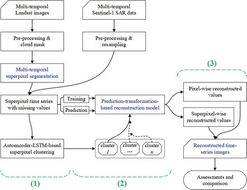
Before the main process, multi-temporal data pre-processing was conducted, which involved the geographic registration, resampling, pixel alignment, and study-area clipping of Landsat images and Sentinel-1A data. In the main step (1), clouds were first manually delineated to produce cloud masks for Landsat images. Then, a modified superpixel algorithm segmented the multi-temporal Landsat images and their masks into superpixels. Once more, superpixel-wise time series with missing values were generated from both multi-temporal Landsat images and Sentinel-1A data. Finally, these superpixel-wise time series were clustered by an AE-LSTM-based unsupervised method into multiple clusters (searching similar superpixels). In the main step (2), for a special cluster, the superpixel-wise time-series set was split into a training sample set and predicting sample set. Moreover, a prediction-transformation-based reconstruction model was built and trained by training samples. In the main step (3), the reconstruction model was applied to superpixel and its pixels to predict superpixel-wise and pixel-wise time-series data, respectively. Then, the superpixel-wise and pixel-wise prediction were fused to produce the final reconstruction results.

2.1. Study area and dataset

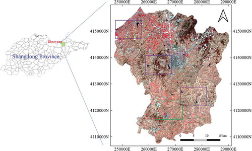
The study area is in the north-eastern region of Shandong Province, China, with central coordinates of 120°23ʹ E and 37°19ʹ N (Figure 2). This region is dominated by a temperate maritime climate, with hot and rainy summer and mild and cool winter. It features mostly plains, and there are some low mountains and hills in middle. The study area covers most landforms and land uses types, including waterbody, forest, farmland, and urban areas, which is suitable to test the proposed method.

Figure 2. The study area in the north-eastern region of Shandong Province, China. The right-hand section presents an overview of the Landsat OLI image acquired on 31 March 2017, with a near-infrared-blue-green band composition. The purple and green boxes, and red line indicate comparison regions and location for further discussions

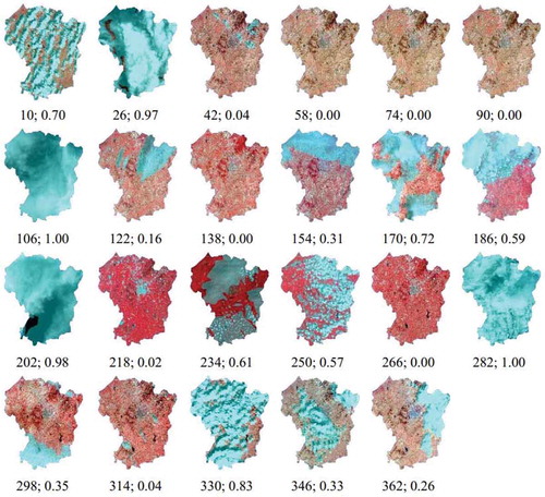
All available 23 Landsat OLI images (hereafter referred to as Landsat images) with Path 120 and Row 34 during 2017 (as listed in Figure 3) were employed to validate the proposed method. Landsat images with a 16-day revisit comprise 7 multi-spectral bands with a spatial resolution of 30 m, from which the widely used blue, green, red, and near-infrared (NIR) bands (band 2 ~ 5) were selected for experiments. All images were obtained at Level 1 G. Among these images, 18 images are contaminated by clouds and shadows. Especially, the image with DOY 106, 282 is totally covered by clouds and shadows.

Figure 3. Multi-temporal Landsat images with cloud mask (with cyan color) in the study area, subfigure represent all the 23 images and the text below the subfigures indicates the acquisition date (in Day of Year) and cloud-covered ratio of the image

All available Sentinel-1A SAR data with a revisit period of 12 days (hereafter referred to as Sentinel-1 data) during 2017 were used as auxiliary data to restore the missing values in Landsat time series. In total, 30 Sentinel-1 ground range detected (GRD) products with Path 11 and Frame 94 in interferometric wide swath imaging model from 9 January 2017 to 23 December 2018 were collected from European Space Agency.

2.2. Data pre-processing and cloud mask

Landsat images were employed as the main data source. Since these data have well-characterized radiometric quality, data pre-processing including geographic registration, pixel alignment, and common-region clipping were conducted. Firstly, a polynomial model with 2 degrees and 9 manually selected and evenly distributed ground control points were employed to geometrically correct the Landsat image to a Google satellite map (produced from Google Tile Map Service with a spatial resolution of 10 m), with registration errors less than 10 m. Secondly, taking an image with DOY 10 as reference, we resampled and aligned the remaining images to match the same pixel grids. Finally, the common regions of the multi-temporal images were clipped for the study area.

Sentinel-1A data were utilized as auxiliary data to reconstruct time-series Landsat images. Since GRD products have thermal noise removed and multi-looked, processing steps including applying precise orbits, calibration, speckle filtering using the enhanced Lee algorithm, terrain correction with the shuttle radar topography mission DEM data with a 90 m spatial resolution were applied to produce intensity images with decibel (dB) scale backscatter coefficient. Then, all intensity images were clipped and geometrically rectified to the Google satellite map using nine manually selected ground control points. Finally, all Sentinel-1A images were resampled and aligned to match the same pixel grids of Landsat images. Here, multi-temporal intensity SAR images with a VH and VV intensity band with a spatial resolution of 30 m were obtained.

Cloud-covered regions were manually delineated as masks for Landsat images. According to the cirrus band and the NIR-red-green composed image (as presented in Figure 3) of Landsat image, we firstly delineated cloud-covered and shadow-covered regions to generate an initial cloud-covered mask. Then, the mask was properly extended to cover the ambiguous pixels around clouds and shadows (which were hardly determined being contaminated or not). Finally, the extended mask was converted into a mask band and appended into the Landsat image.

2.3. Multi-temporal superpixel segmentation

Superpixel is a perceptually meaningful atomic region, comprising interconnected similar pixels on images. It captures image redundancy and provides a convenient primitive for computing image features, and greatly reduce the complexity of subsequent image processing tasks (Achanta et al. 2012). So, superpixel has become an essential tool for many vision algorithms. In this study, we introduced superpixels to suppress image noise, and systematically reduce cover-type errors in reconstruction (Wu et al. 2018). Many approaches are proposed to produce superpixels, such as SEEDS (Van den Bergh et al. 2015), SLIC (Achanta et al. 2012), and SSN (Jampani, Sun, and M Y et al. 2018). Among these algorithms, SLIC is faster and more memory efficient, is easy to use and straightforward to extend to higher dimensions. So, it was modified to produce superpixels, on the multi-temporal Landsat images.

Original SLIC is designed for three-band fully covered images. To apply the SLIC algorithm onto multi-temporal masked images, several tricks were adopted. Firstly, being prior boundaries, cloud masks split image region into multiple sub-regions, in which a superpixel algorithm was carried out. Secondly, since the Lab color space is not suitable for multi-temporal multi-spectral images, we directly input all bands equally into SLIC. Thirdly, we used the parameter “superpixel size” instead of “number of superpixels” to adapt to image regions with various sizes. In this study, the values for SLIC parameters “superpixel size,” “trade-off coefficient between spectral similarity and spatial similarity,” and “number of iterations” were set to 15, 10, 10, respectively, for better performance. It is noted that no post-processing was applied to eliminate small regions, to ensure any superpixel being fully covered by a cloud mask. Approximate 56,000 superpixels were produced in the study area.

2.4. Superpixel-wise time series and clustering

2.4.1. Superpixel-wise time series

According to the multi-temporal superpixel segmentation, the mask band m can indicate whether a superpixel p is fully cloud-covered or not. To produce superpixel-wise time-series curves, we first defined the masked superpixel value lmp of the j ($1\le j\le T_L$$1\le j\le T_L$) time step (T_L is the number of time steps), in the i ($1\le i\le B_L$$1\le i\le B_L$) Landsat band (B_L is the number of bands) for the k superpixel as:

$lm{p}_k^{i,j}=\left\{\begin{array}{c}{p}_k^{i,j},if{m}_k^j=0\\ mv,if{m}_k^j=1\end{array}\right.$$lm{p}_k^{i,j}=\left\{\begin{array}{c}{p}_k^{i,j},if{m}_k^j=0\\ mv,if{m}_k^j=1\end{array}\right.$

where $p_k^{i,j}$$p_k^{i,j}$ is the mean pixel value of the k superpixel of the j time step in the i band, mv is the masking value (a value much more than the biggest pixel value, and we set it to be 19,999 in this study) in time-series curves, indicating a missing value caused by clouds. Then, we constructed superpixel-wise time-series LTS for the i band for the k superpixel as

$LT{S}_k^{i,}=\left[lm{p}_k^{i,1},lm{p}_k^{i,2},\dots ,lm{p}_k^{i,T_L}\right]$$LT{S}_k^{i,}=\left[lm{p}_k^{i,1},lm{p}_k^{i,2},\dots ,lm{p}_k^{i,T_L}\right]$

.

Following the similar procedure, we constructed superpixel-wise time-series curves for the i band for the k superpixel for Sentinel-1 intensity images as

$ST{S}_k^{i,}=\left[s{p}_k^{i,1},s{p}_k^{i,2},\dots ,s{p}_k^{i,T_S}\right]$$ST{S}_k^{i,}=\left[s{p}_k^{i,1},s{p}_k^{i,2},\dots ,s{p}_k^{i,T_S}\right]$

,

where $s{p}_k^{i,j}$$s{p}_k^{i,j}$ is the mean pixel value of the k superpixel of the j ($1\le j\le T_S$$1\le j\le T_S$) time step (T_S is the number of time steps), in the i ($1\le i\le 2$$1\le i\le 2$) Sentinel-1 intensity band (B_S is the number of bands) for the k superpixel.

Finally, time-series curves for the k superpixel were constructed as:

$\begin{array}{rl}& T{S}_k=\left[LT{S}_k,ST{S}_k\right]\\ & =\left[\begin{array}{c}\begin{array}{cccc}lm{p}_k^{1,1}& lm{p}_k^{1,2}& \cdots & lm{p}_k^{1,T_L}\end{array}\\ \begin{array}{cccc}lm{p}_k^{2,1}& lm{p}_k^{2,2}& \cdots & lm{p}_k^{2,T_L}\end{array},\begin{array}{cc}s{p}_k^{1,1}& s{p}_k^{1,2}\\ s{p}_k^{2,1}& s{p}_k^{2,2}\end{array}\begin{array}{cc}\cdots & s{p}_k^{1,T_S}\\ \cdots & s{p}_k^{2,T_S}\end{array}\\ ⋮\\ \begin{array}{cccc}lm{p}_k^{B_L,1}& lm{p}_k^{B_L,2}& \dots & lm{p}_k^{B_L,T_L}\end{array}\end{array}\right]\end{array}$$\begin{array}{rl}& T{S}_k=\left[LT{S}_k,ST{S}_k\right]\\ & =\left[\begin{array}{c}\begin{array}{cccc}lm{p}_k^{1,1}& lm{p}_k^{1,2}& \cdots & lm{p}_k^{1,T_L}\end{array}\\ \begin{array}{cccc}lm{p}_k^{2,1}& lm{p}_k^{2,2}& \cdots & lm{p}_k^{2,T_L}\end{array},\begin{array}{cc}s{p}_k^{1,1}& s{p}_k^{1,2}\\ s{p}_k^{2,1}& s{p}_k^{2,2}\end{array}\begin{array}{cc}\cdots & s{p}_k^{1,T_S}\\ \cdots & s{p}_k^{2,T_S}\end{array}\\ ⋮\\ \begin{array}{cccc}lm{p}_k^{B_L,1}& lm{p}_k^{B_L,2}& \dots & lm{p}_k^{B_L,T_L}\end{array}\end{array}\right]\end{array}$

2.4.2. Superpixel clustering

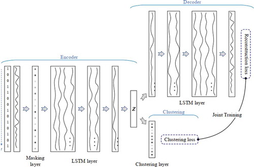
An AE-LSTM-based network was employed for clustering time-series data with missing values (masked pixels), as shown in Figure 4. In the AE-LSTM-based framework for time-series clustering, we firstly fed pixel-wise time-series $\left[LT{S}_k^{1,},LT{S}_k^{2,},\dots ,LT{S}_k^{B,}\right]$$\left[LT{S}_k^{1,},LT{S}_k^{2,},\dots ,LT{S}_k^{B,}\right]$ into a masking layer and a stacked LSTM network (with four LSTM layers) to produce the latent high-level features z of input time-series data (referred to as encoder). Then, on one hand, the latent features z were fed into another stacked LSTM network (with four LSTM layers) to produce reconstructions (referred to as decoder), under the constraints of reconstruction loss; on the other hand, the latent features z were fed into a clustering layer to calculate clustering probabilities of the latent features (referred to as clustering), under the constraints of clustering loss. Finally, the reconstruction loss and the clustering loss were fused for joint training, as, where $L_r$$L_r$ and $L_c$$L_c$ are reconstruction loss and clustering loss, respectively, and $\alpha \ge 0$$\alpha \ge 0$ is the coefficient of clustering loss, to balance $L_r$$L_r$ and $L_c$$L_c$.

The clustering loss (Xie, Girshick, and Farhadi 2016) is defined as KL divergence (measuring the non-symmetric difference) between distributions P and Q, where Q is the distribution of soft labels measured by Student’s t-distribution and P is the target distribution derived from Q. So, the clustering loss is defined as

$L_c=KL\left(P||Q\right)=\sum _i\sum _j{p}_{ij}log\frac{p_{ij}}{q_{ij}}$$L_c=KL\left(P||Q\right)=\sum _i\sum _j{p}_{ij}log\frac{p_{ij}}{q_{ij}}$

$q_{ij}=\frac{{\left(1+{∥z_i-{\mu }_j∥}^2\right)}^{-1}}{{\sum }_j{\left(1+{∥z_i-{\mu }_j∥}^2\right)}^{-1}}$$q_{ij}=\frac{{\left(1+{∥z_i-{\mu }_j∥}^2\right)}^{-1}}{{\sum }_j{\left(1+{∥z_i-{\mu }_j∥}^2\right)}^{-1}}$

$p_{ij}=\frac{q_{ij}^2/{\sum }_i{q}_{ij}}{{\sum }_j\left(q_{ij}^2/{\sum }_i{q}_{ij}\right)}$$p_{ij}=\frac{q_{ij}^2/{\sum }_i{q}_{ij}}{{\sum }_j\left(q_{ij}^2/{\sum }_i{q}_{ij}\right)}$

where $p_{ij}$$p_{ij}$ is target distribution, $q_{ij}$$q_{ij}$ is the similarity between latent features z and cluster center $\mu$$\mu$ measured by Student’s t-distribution.

The reconstruction loss is measured by mean squared error:

$L_r=\frac{1}{n}\sum _{i=1}^n{∥x_i-g\left(f\left(x_i\right)\right)∥}^2$$L_r=\frac{1}{n}\sum _{i=1}^n{∥x_i-g\left(f\left(x_i\right)\right)∥}^2$

where f and g are encoder and decoder mappings, respectively. More details can be found in (Xie, Girshick, and Farhadi 2016).

Figure 4. AE-LSTM-based network for clustering time-series data with missing values

In detail, we set the number of hidden neurons of LSTM layers to be 32, and the coefficient of clustering loss $\alpha$$\alpha$ to be its default value 0.1. The number of clusters is a hyperparameter. On one hand, more clusters may improve the homogeneity of clusters, facilitating reconstruction; on the other hand, too many clusters would reduce the pixel numbers in clusters, hampering training reconstruction models. In this study, we set it to be 8, which was found to produce better results.

2.5. Prediction-transformation-based time-series reconstruction

In this study, both Landsat images and Sentinel-1 data were used to restore the missing values in Landsat time series. Incorporating intrinsic tendency and prediction information from Landsat images and mapping and transformation from SAR data, a prediction-transformation-based LSTM network was designed to predict missing values for Landsat time-series images, as presented in Figure 5 (all processing modules were used for training, but only modules with solid box lines were employed for predicting).

Figure 5. Prediction-transformation-fusion network for restoring missing values in time series

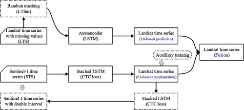
The upper part is Landsat-based (L8-based) prediction and reconstruction. Firstly, from superpixel-wise time-series TS, we fetched the Landsat time-series LTS and randomly masked several (usually set to be 1, 2, or 3) steps to be masking value mv. Secondly, the masked Landsat time-series LTSm was fed into an LSTM-based autoencoder network to produce L8-based prediction. The lower part is Sentinel-1-based (S1-based) transformation and reconstruction. Since the imaging date and cycle are different between Landsat images and Sentinel-1 data, we employed a connectionist temporal classification (CTC) loss (Graves, Fernández, and Gomez et al. 2006), instead of mean squared loss or sum squared loss in traditional autoencoder network. Firstly, the Sentinel-1 time-series STS was fed into a stacked LSTM network to produce a Sentinel-1-retrieved time-series features, called S1-based transformation (encoder step in an autoencoder). Secondly, an auxiliary training was added to guide the S1-based transformation to be equal to the input Landsat time-series LTS. Thirdly, the S1-based transformation was fed into another stacked LSTM network to restore the input time-series STS. In the fusion stage, a linear layer was firstly applied to the L8-based prediction to produce a weighted prediction. Then, the weighted prediction and the S1-based transformation were concatenated and fed into another linear layer to produce the final reconstruction results.

In detail, in the staked LSTM network, four LSTM layers with 32 hidden neurons were stacked to transfer raw time-series curves into high-level features. The length of the intermediate time-series feature is eight times that of the final time series, respectively.

2.5.1. Denoise autoencoder

An autoencoder is a neural network used for feature selection and extraction. While it will run the risk of learning the identity function (the output simply equals the input), when with more hidden layers than inputs, which is useless (Vincent, Larochelle, and Bengio et al. 2008). Denoising autoencoders were proposed to address the identity-function risk through randomly corrupting input (i.e. introducing noise). In the decoding stage, a denoising autoencoder tries to undo the effect of a corruption process stochastically applied to the input (Zhao et al. 2018). More details can be found in (Vincent, Larochelle, and Lajoie et al. 2010).

In this study, we employed denoising autoencoder networks to capture the intrinsic statistical dependencies to restore the missing data in the Landsat retrieved time series. Following the stochastic corruption process, we randomly set some of the entries of the input to the masking value. And the number of total masked entries is as many as half of them, to ensure the reliability of recovery results.

2.5.2. Connectionist temporal classification loss

In this study, the revisit period of Sentinel-1 satellite (12 days) is shorter than that of Landsat satellite (16 days), and there is not a consistent one-to-one match from Sentinel-1 data to Landsat images. So, to calculate the reconstruction error from Sentinel-1 to Landsat time series, a CTC loss was employed.

The CTC is a type of neural network output and is associated with scoring function, for training recurrent neural networks such as LSTM networks. Different from other loss functions, CTC is alignment-free and does not require an alignment between the input and the output. CTC works by summing over the probability of all possible alignments between time series to get the probability of an output given an input, which is widely used for recognizing phonemes in speech audio (Salazar, Kirchhoff, and Huang 2019). Furthermore, the other requirement of the CTC loss is the number of entries of outputs can only be less than that of inputs. So, we just used the half time-series (with double intervals) in the decoding stage of the lower part in Figure 5.

2.5.3. Auxiliary training

Auxiliary training is a useful trick in deep learning to accelerate the training process (Liu, Zhuang, and Shen et al. 2019). In this study, in addition to improving training efficiency, we try to employ the auxiliary training to guide the intermediate representation of the autoencoder network as similar as possible with the Landsat time series, in which Landsat time-series LTS was taken as targets.

2.5.4. Training and predicting

To ensure the training performance (Vincent, Larochelle, and Lajoie et al. 2010), superpixels with a clear ratio greater than 0.55 in Landsat time series were selected for training reconstruction models. All superpixels with missing data were restored using trained models.

When training, the input LTS and STS were fed into the upper part and lower part, and processed by all processing modules in Figure 5. When predicting, we directly fed LTS and STS into the denoised autoencoder network and the encoder stage of the autoencoder network (skipping modules with dotted box lines), to produce the final reconstruction.

2.6. Superpixel-wise and pixel-wise fusion

Superpixel was used to reduce pixel-wise noise and extract more robust time-series features. But superpixel also suppresses pixel characteristics, making all pixels in a superpixel sharing the same reconstruction values. The superpixel-wise reconstruction represents the general features of regions, and the pixel-wise reveals the local characteristics of pixels. So, a method was designed to fuse the superpixel-wise and pixel-wise reconstruction together. Firstly, the trained reconstruction model was applied on a superpixel TSsp to produce superpixel-wise reconstruction time-series RTSsp. Then, the reconstruction model was applied on every pixel TSp in the superpixel to produce a pixel-wise time-series RTSp. Finally, a weighted sum was used to fuse the RTSsp and RTSp together to produce the final reconstruction FTS for pixels.

$FTS=s\ast RT{S}_{sp}+\left(1-s\right)\ast RT{S}_p$$FTS=s\ast RT{S}_{sp}+\left(1-s\right)\ast RT{S}_p$

$s=COR\left(TSsp,TSp\right)$$s=COR\left(TSsp,TSp\right)$

where s indicates the time-series similarity between superpixel-wise and pixel-wise time series, using the simple Pearson Correlation Coefficient in our study.

2.7. Performance evaluation

2.7.1. Comparative methods

To make a comparative analysis, the proposed superpixel-based prediction-transformation-fusion (SPTF-based) method was compared with the state-of-the-art methods of spatially and temporally weighted regression (STWR-based) method (Chen, Huang, and Chen et al. 2016), spectral–temporal patch-based missing area reconstruction (STP-based) (Wu et al. 2018), and patch-based contextualized autoencoder neural network (PCAE-based) method (Malek et al. 2018).

The STWR-based method optimally integrates both spatial and temporal information in time-series scenes to restore missing pixels using spatially and temporally weighted regression and inverse distance weighted interpolator, which is selected as a traditional geostatistical method for experimental comparison. The STP-based method takes spectral-temporal patches as basic units for searching similar structures and injecting textural information to preserve spatial and spectral continuities, and suppress salt-and-pepper noises and false edges, which is selected as a patch-based method for experimental comparison. The PCAE-based method employs an autoencoder neural network to calculate the transformation function from the cloud-free reference to the target images, to restore missing pixels for multispectral images, which is selected as a deep-learning-based approach for experimental comparison.

2.7.2. Evaluation metrics

Reconstruction performance was evaluated by simulated cloud-covered images, which has the advantage of assessing the reconstruction against actual observed data. Firstly, we randomly masked cloud-free values from time-series curves of Landsat images to generate the simulated cloud-covered images. Then, we compared the reconstructed pixels with the actual pixels in the simulated regions pixel-by-pixel, to calculate reconstruction accuracy.

For pixel i with an actual value $x_i$$x_i$ at a special band, we restored it to be predicted value ${\hat{x}}_i$${\hat{x}}_i$. Its reconstruction error can be calculated as $e_i=\left|x_i-{\hat{x}}_i\right|$$e_i=\left|x_i-{\hat{x}}_i\right|$. The smaller the value of e, the higher the accuracy. For the total reconstruction accuracy of cloud-covered regions, we adopted the normalized mean square error (NMSE) index, mean absolute error (MAE) index, mean absolute percentage error (MAPE) index, and correlation coefficient (CC) index for quantitative evaluation.

$\mathrm{N}\mathrm{M}\mathrm{S}\mathrm{E}=\frac{1}{N}\sum _{i\in R}\frac{{\left(x_i-{\hat{x}}_i\right)}^2}{u\left(x\right)u\left(\hat{x}\right)}$$\mathrm{N}\mathrm{M}\mathrm{S}\mathrm{E}=\frac{1}{N}\sum _{i\in R}\frac{{\left(x_i-{\hat{x}}_i\right)}^2}{u\left(x\right)u\left(\hat{x}\right)}$

$MAE=\frac{1}{N}\sum _{i\in R}\left|x_i-{\hat{x}}_i\right|$$MAE=\frac{1}{N}\sum _{i\in R}\left|x_i-{\hat{x}}_i\right|$

$MAPE=\frac{1}{N}\sum _{i\in R}\left|x_i-{\hat{x}}_i\right|/x_i$$MAPE=\frac{1}{N}\sum _{i\in R}\left|x_i-{\hat{x}}_i\right|/x_i$

$\mathrm{C}\mathrm{C}=\frac{{\sum }_{i\in R}\left(x_i-u\left(x_i\right)\right)\left({\hat{x}}_i-u\left({\hat{x}}_i\right)\right)}{\sqrt{{\sum }_{i\in R}{\left(x_i-u\left(x\right)\right)}^2{\sum }_{i\in R}{\left({\hat{x}}_i-u\left(\hat{x}\right)\right)}^2}}$$\mathrm{C}\mathrm{C}=\frac{{\sum }_{i\in R}\left(x_i-u\left(x_i\right)\right)\left({\hat{x}}_i-u\left({\hat{x}}_i\right)\right)}{\sqrt{{\sum }_{i\in R}{\left(x_i-u\left(x\right)\right)}^2{\sum }_{i\in R}{\left({\hat{x}}_i-u\left(\hat{x}\right)\right)}^2}}$

where N is the total number of missing pixels in cloud-covered region R, $u\left(x\right)$$u\left(x\right)$ and $u\left(\hat{x}\right)$$u\left(\hat{x}\right)$ are the mean values of the actual and the reconstructed values in R, respectively.

NMSE indicates the deviation between the actual observation and the reconstructed results, MAE reflects the actual errors of predicted values, MAPE provides a measure of relative comparison even when data vary in magnitude. CC depicts the textural similarity between the actual observation and the recovered result. For NMSE, MAE, and MAPE, lower values indicate better reconstruction and are preferable. A larger CC indicates a closer consistency between the regions of data.

All the above indexes were defined for reconstruction at a special time step. In our study, we reconstructed the whole time series all at once. So, we employed the average score of evaluation indexes (e.g. NMSE) at all cloud-free time steps to evaluate the reconstruction performance for the whole time series.

3. Experiments and discussion

Using multi-temporal Landsat images and Sentinel-1 data, experiments were carried out to test the effectiveness and efficiency of the proposed method, compared to three state-of-the-art methods. Accuracy assessments were conducted on the reconstruction results of time-series images to discuss the promotion of the proposed model over the comparative methods, the effectiveness of the prediction-transformation-fusion reconstruction model and pixel-superpixel fusion, and reconstruction performance for various land-cover types.

3.1. Reconstruction

Following subsection 2.5, trained models using approximate 36,000 superpixels (80% of training samples) were employed to restore cloud-covered time-series images. The time-series reconstructed images (using the NIR-red-green band composition) produced by the proposed SPTF-based method are presented in Figure 6. Since images of DOY 42 (20170211), 58 (20170227), 74 (20170315), 90 (20170331), 138 (20170518), 218 (20170806), 266 (20170923), and 314 (20171110) have no or small cloud-covered regions, their reconstruction results were not demonstrated.

Figure 6. Reconstruction results of cloud-covered Landsat image by the proposed method, subfigures (a-p) represent the reconstructed images in the NIR-red-green band composition, and the text below the image indicates the imaging dates

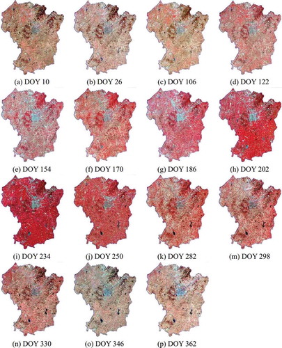
As a whole, the multi-temporal reconstructed images can demonstrate the landscape dynamic process of the study area. In the NIR-red-green composition, through the NIR band, the annual change in vegetation was watched. From Jan. to Aug., as vegetation flourishes, images become redder. While from Aug. to Dec., vegetation is declining with red fading from images. For any image in time series (especially the fully cloud-covered images, such as images with DOY 106 and 282), the proposed method has restored missing data for cloud-covered regions with various cloud-covered ratios and distribution positions, producing visually plausible cloud-free images. Taking a close look at local regions of reconstructed images, we found out that the proposed method also captured the unusual changes in the reservoir at the right bottom of the study area. Because of the severe drought in 2017, from Jan. to Jul., the reservoir gradually shrank to almost disappear (rarely happening in other years), and from Aug, the reservoir reappeared suddenly. Furthermore, we observed that there was some spectral distortion (color imbalance between the upper half and the lower half) in the reconstructed image with DOY 202. The possible reason was that the cloud-covered ratio of 0.97 was too big to provide enough information for reconstructing cloud-covered regions.

3.2. Comparison and evaluation

3.2.1. Visual comparison

For comparisons, the three state-of-the-art reconstruction methods (the STWR-based, STP-based, and PCAE-based methods) were applied to the experimental data to restore missing data in cloud-covered regions. Since the STWR-based and STP-based methods were multi-temporal based, the whole Landsat time series were used to reconstruct the target images. In the PCAE-based method, the Landsat image with a closer acquired date to that of the image to be reconstructed was taken as the reference image. For example, the image with DOY 234 was referred to the image with DOY 266. Reconstructed images in the purple boxes in Figure 2 with DOY 74 (cloud-covered ratio 0.00), 154 (cloud-covered ratio 0.31), and 234 (cloud-covered ratio 0.61) are presented in Figure 7.

Figure 7. Sub results of missing data reconstruction in the comparative experiments. Panel A list the actual cloud-free Landsat images (in the NIR-red-green band composition) acquired on March 15, June 3, and September 7, in 2017, in which green boxes indicate comparison regions with obviously different reconstructions. Panel B-E list the corresponding reconstruction results using the STWR-based, STP-based, PCAE-based, and the proposed SPTF-based methods, respectively

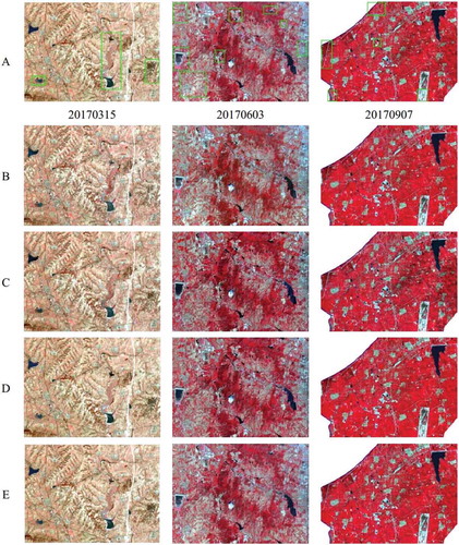
Generally, all comparative methods and the proposed method yielded visually plausible images, compared to the actual observation. With a close comparison with the actual cloud-free images (regions marked by green boxes), the proposed method can capture and model the scene change over time. Our restored results were shown to be quite similar to the actual ones in both spatial details and spectral comparability.

3.2.2. Quantitative evaluation

To quantitatively evaluate the reconstruction performance of the proposed SPTF-based approach (comparing with the STWR-based, STP-based, and PCAE-based methods), we carried out four experiments to reconstruct the whole time-series curves. When calculating evaluation metrics, approximate 9000 pixels or superpixels with a cloud-covered ratio less than 0.40 were firstly randomly selected. Then, two randomly selected time steps were masked to generate simulated cloud-covered images. Finally, the restored time-series were accessed, compared with the simulated images. The accuracy assessment of reconstruction results is listed in Table 1, in which IR (improvement ratio) evaluates the degree of the improvement of the proposed method with respect to the best comparative results.

Table 1. Accuracy assessment of reconstruction results from the proposed and three comparative methods

		STWR	STP	PCAE	SPTF	IR (%)
Blue	NMSE	2.2118	2.0880	2.0829	1.5105	37.30
	MAE	45.0503	47.6752	42.2403	38.2474	10.44
	MAPE	9.6537	9.6444	8.9290	7.7682	14.94
	CC	0.8990	0.8803	0.9146	0.9365	2.34
Green	NMSE	1.0154	1.2011	0.9621	0.7325	30.73
	MAE	53.5537	55.9831	49.1739	39.1270	25.68
	MAPE	6.9234	7.3324	6.5663	5.8787	11.70
	CC	0.9163	0.8760	0.9312	0.9398	0.92
Red	NMSE	2.7711	2.9832	2.4311	1.8080	34.46
	MAE	88.0787	88.5734	73.2295	55.1159	32.86
	MAPE	10.2945	10.4388	10.1848	9.4731	7.51
	CC	0.8754	0.8369	0.9016	0.9218	2.24
Nir	NMSE	22.2710	20.2986	19.9271	14.3878	38.50
	MAE	169.1427	173.6974	150.7713	124.7914	20.82
	MAPE	31.7492	31.2351	29.7785	24.9473	19.37
	CC	0.7917	0.8098	0.8237	0.8574	4.09

On the whole, the SPTF-based method achieved the best reconstruction accuracy, compared with the three state-of-the-art methods. This was expected, because the proposed method took the time series as a whole when learning the change rules and predicting missing data in time-series curves. When comparing to the PCAE-based method (using one reference image), the SPTF-based method extracted and incorporated more scene change information from the multi-temporal images to construct prediction models and to restore missing data in time series. When comparing to the STWR-based and STP-based methods, the SPTF-based method used AE and LSTM networks to learn deeper and nonlinear time-series information to capture the scene change patterns. Furthermore, reconstruction accuracies of the SPTF-based method varied greatly in various spectral bands. The green band presented the best reconstruction accuracies (0.7325 in the NMSE, 39.1270 in the MAE, 5.88% in MAPE, and 0.94 in CC), followed by the blue and red bands, and the NIR band produced the worst results. This was consistent with the results of previous studies (Chen, Huang, and Chen et al. 2016). On one hand, clouds make the greatest impact on the blue band with the shortest wavelength. On the other hand, red band and NIR band mainly demonstrate more complex temporal tendency information of vegetation growth, which is hard to precisely capture by reconstruction models.

It was also noted that the four bands produced various promotions. On one hand, in both previous studies and our study, the green band produced the best reconstruction, and the restored values were most similar to the ground truth. So, it was hard to further achieve great improvement, for the green band. Thus, the blue band achieved the smallest promotion (with 31%, 26%, 12%, 1% IR in the NMSE, MAE, MAPE, and CC, respectively). On the other hand, compared to the previous studies, we deeply extracted and utilized the temporal tendency to restore missing data, using LSTM networks. And this temporal tendency mainly expressed in vegetation annual change and the NIR band. Thus, the SPTF-based method achieved the greatest promotion in the NIR band (with 38%, 20%, 19%, 4% IR in the NMSE, MAE, MAPE, and CC, respectively). It further indicated the proposed method could extract and model the vegetation tendency and change patterns, compared to the comparative methods.

3.3. Discussion

To further understand the performance of the SPTF-based method, we conducted a series of experiments to discuss whether the fusion between L8-based prediction and S1-based transformation was useful, whether the fusion between pixel-wise and superpixel-wise reconstruction was effective, and reconstruction performance on various land-cover types.

3.3.1. Advantages of prediction-transformation-fusion

In this study, a prediction-transformation-fusion model was designed to incorporate intrinsic tendency information in time-series optical images and transformation from SAR data. Here, we carried out a comparative experiment to test the advantage of the prediction-transformation-fusion model over a prediction and a transformation model (as presented in Figure 5, just using the upper or lower part, respectively). Following the same evaluation procedure in subsection 3.2.2, evaluation matrices of reconstruction results produced from the three models were calculated and presented in Table 2.

Table 2. Accuracy assessment of reconstruction results produced from the prediction, transformation, and prediction-transformation-fusion models

	L8-based				S1-based				Fusion
	NMSE	MAE	MAPE	CC	NMSE	MAE	MAPE	CC	NMSE	MAE	MAPE	CC
Blue	1.8105	40.9474	8.6682	0.9065	3.1082	49.1984	11.3199	0.8629	1.5238	37.8258	7.7595	0.9361
Green	0.8325	43.1270	6.1787	0.9247	1.4031	50.8478	7.8052	0.8813	0.7430	38.2681	5.7913	0.9438
Red	1.9380	60.9511	9.5731	0.9105	3.5919	77.4116	14.0367	0.8392	1.7954	54.1535	9.3649	0.9213
Nir	18.3878	130.7914	27.9473	0.8427	27.7765	166.7985	33.6725	0.7834	14.9093	124.6282	24.6896	0.8524

Generally, the prediction-transformation fusion model achieved the best performance, in all evaluation index, for all spectral bands, compared to the prediction and transformation models. This was expected since the prediction-transformation-fusion model can incorporate the prediction information from the Landsat time series and the transformation information from Sentinel-1 time series to model the landscape change pattern for reconstructing missing data. Further, we found out that the L8-based prediction reconstruction obtained better results than the S1-based transformation reconstruction. We argued that in the L8-based prediction reconstruction, information expression is consistent from the source to the target images, which ensures better performance, while the effectiveness of transformation from SAR data to optical images limited the S1-based reconstruction performance. Even so, SAR data are needful to restore fully cloud-covered images and improve reconstruction.

Furthermore, the 9000 testing samples were randomly divided into 900 groups. Then, we randomly selected 50 groups to calculate their mean matrices in groups. Finally, T-tests with hypotheses of no difference between comparison pairs were applied on the matric lists to compare the difference of the statistical significance between the reconstruction of the three models. Table 3 presents the statistical P-values of the T-test on reconstruction accuracy differences, in the green band. Considering that reconstructions from the fusion model are better than that from the L8-based and S1-based models in Table 2, P-values much less than 0.05 (rejecting the null hypotheses) further highlight the obvious performance differences among three reconstructions, and the efficiency of the L8-S1-fusion model compared with the L8-based and S1-based models.

Table 3. T-test for performance difference of reconstruction from the L8-based, S1-based, and fusion models

	P-valueNMSE	P-valueMAE	P-valueMAPE
L8-based vs. Fusion	2.97E-03	1.03E-02	2.55E-02
S1-based vs. Fusion	3.94E-04	7.71E-09	2.05E-05
L8-based vs. S1-based	6.21E-04	1.41E-06	1.97E-04

3.3.2. Advantages of superpixel-wise and pixel-wise fusion

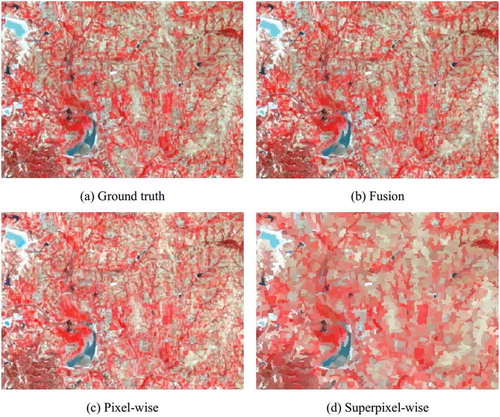
Compared with previous studies, our study fused pixel-wise and superpixel-wise reconstruction, to eliminate systematic land-type errors and keep pixel-wise features in a superpixel. In this study, we carried out a comparative experiment to evaluate the improvement of fusion, compared to the pixel-wise and superpixel-wise reconstruction. We followed the process in Section 2.6 and Figure 2, for the superpixel-wise and pixel-wise fusion. While in the pixel-wise or the superpixel-wise experiments, we just taken the pixel-wise or superpixel-wise reconstruction in Figure 2 as the final results, respectively. Figure 8 presents the reconstruction results in the green box in Figure 2 on the target image with DOY 138, from the pixel-wise, superpixel-wise, and fusion-wise models.

Figure 8. Ground truth image and corresponding reconstruction results from the pixel-wise, superpixel-wise, and fusion-wise models

To quantitatively evaluate the advantage of fusion-wise reconstruction over pixel-wise reconstruction, we extracted their horizontal profiles of ground truth and reconstructions of the green band in the middle of the study area (the red horizontal line in Figure 2), as presented in Figure 9.

Figure 9. Horizontal profiles of ground truth and reconstructions from the pixel-wise, superpixel-wise, and fusion models in the middle of study area, in the green bands

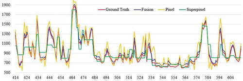
On the whole (in Figure 8), pixel-wise reconstruction seemed to be able to restore the ground truth, from the perspective of visual effect, while, in some local regions (e.g. water areas in the left top corner in Figure 8), pixel-wise reconstruction failed to capture entirety of superpixels. Since only mean curves of time series were restored for superpixels, superpixel-wise reconstruction demonstrates obvious patch-like homogeneity and hard boundaries between patches. Fusion-wise reconstruction not only reduces systematic errors from land-cover types but also keeps characteristic for pixels, achieving the best performance. These results also represent in the horizontal profile curves in Figure 9. The pixel-wise profile presents minimum and maximum values, while the superpixel-wise profile shows the regional average. The fusion-wise profile incorporates the superpixel-wise and pixel-wise profiles, being closer to the ground truth profile.

3.3.3. Error distributions via land-cover types

Various land-cover types present different change patterns in multi-temporal images and different sensitivities to cloud covering (Wu et al. 2018). In this experiment, we attempted to assess the reconstruction performance of the proposed method for typical land-cover types (including water, forest, farmland, and urban area). Taking the image with DOY 266 as the target, we firstly randomly removed some patches (covering a typical land cover, such as urban area) to simulate cloud-covered regions. Then, we employed SPTF-based models to restore the cloud-covered regions. Finally, we compared the actual image (ground truth) with the reconstructed results pixel by pixel, to calculate error distributions (sum of errors from four bands). Figure 10 presents the local ground truth images and corresponding reconstruction results, and normalized (with the maximum and minimum error values, to the range [0,255]) error distribution (boundaries of water, forest, and urban area were delineated for clear comparison, while farmland was too fragmentary to be delineated on the Landsat image).

Figure 10. Reconstruction error distributions for typical land-cover types

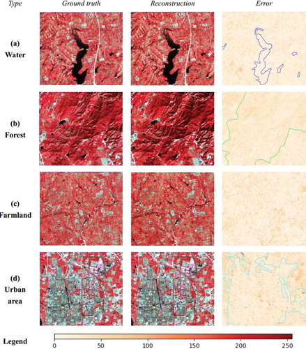
In Figure 10, the proposed method produced greater reconstruction errors for artificial objects (farmland and urban area) than natural objects (water and forest). Specifically, the water area (the first row in Figure 10) presented smaller and uniform reconstruction errors, with a mean 22.49 and a standard (std.) 6.23. Since waterbody appeared low spectral radiance in satellite images and small changes during 1 year, the proposed method generated smaller absolute errors for water areas. Forest (the second row in Figure 10) is largely affected by the phenological cycle, which was captured by the proposed method using multi-temporal data. Furthermore, it is homogeneous in spectral band due to less affected by human activities. Thus, it shows smaller reconstruction errors (with a mean 38.72 and a std. 10.31), compared to farmland and urban area. Further analysis showed that error distribution of forest followed special law under the impact of microtopography (local aspects and slopes). We argued that local topography has a systematical effect in SAR imaging, and then propagates into reconstruction results of forest areas. In theory, mainly dominated by the phenological cycle of vegetation, farmland (the third row in Figure 10) should present a similar error distribution with forest. However, farmland is artificial, and agricultural activities (e.g. multiple cropping) would change or even destroy the temporal tendency of vegetation. Thus, farmland presented greater reconstruction error, with a mean 52.73 and a std. 14.21. Different from previous studies, our reconstruction did not present larger errors in urban areas (the fourth row in Figure 10, with a mean 48.16 and a std. 15.97), except for some small development areas. What is more, road areas showed a good reconstruction, even better than farmland. On one hand, urban areas stay the same or have a few changes in 1 year, which is easy to express in multi-temporal data. On the other hand, the proposed method employed SAR data to describe spatial structures of urban objects (e.g. buildings), improving reconstruction performance in urban areas.

3.4. More experiments

To further test the proposed method for other study area, we carried out another experiment on Jintan District, Jiangsu Province, China. The west is dominated by mountains, and the east is a flat plain. The area is dominated by the subtropical monsoon climate, with plenty of rainfall and sunshine, favorable for growing vegetation. Such a humid weather pattern caused more and larger cloud-covered regions, and a higher cloud-covered ratio, in multi-temporal Landsat images, than that in Zhaoyuan. We collected all 23 Landsat images and 30 Sentinel-1A GRD products in 2018, and produced approximately 30,000 superpixels in the study area. Following the same procedures, we have restored cloud-covered regions in the time-series Landsat images. Reconstruction results with different cloud-covered ratios (11% for DOY 278, 43% for DOY 134, 52% for DOY 198, and 79% for DOY 70) are presented in Figure 11.

Figure 11. Reconstruction results of the time-series Landsat images for Jintan using the proposed method (cloud-covered masks on the top right), and the text below the image indicates the imaging dates and cloud-covered ratios

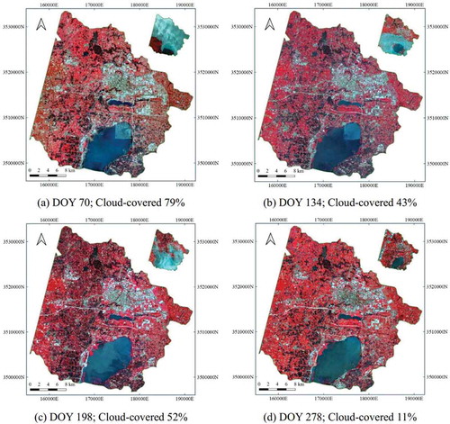
Overall, the proposed method has restored missing data for Landsat images with various cloud-covered regions. The restored results appeared good visual effects, presenting the changes in vegetation. On DOY 70, vegetation began to grow, showing light red in the NIR-red-green composed images (Figure 7(a)). On DOY 134 and 198 (Figure 7(b and c)), the vegetation became flourishing, with stronger vegetation information in the west forest areas. Thus, we argued that this experiment further verified the availability for time-series reconstruction of the proposed method.

4. Conclusion

Time-series reconstruction for cloud/shadow-covered optical images is greatly important for enhancing the data availability and temporal analysis. We proposed a superpixel-based time-series reconstruction method for optical images incorporating SAR data using autoencoder networks, through the incorporation between intrinsic tendency and prediction information in time-series optical images, and mapping and transformation from SAR data. The method was validated onto two datasets of multi-temporal cloud-covered Landsat images and Sentinel-1 data. The reconstruction results, showing a greater improvement relative to the state-of-the-art methods, demonstrated the effectiveness of the proposed method for reconstructing time-series satellite images. From further discussions on the effectiveness of the prediction-transformation-fusion reconstruction model and pixel-superpixel fusion, and reconstruction performance for various land-cover types, this study concludes: (1) the prediction-transformation-fusion reconstruction model presents better results, compared to the prediction and transformation models; (2) pixel-superpixel fusion could reduce systematic errors from land-cover types as well as keep characteristic for pixels; (3) the reconstruction method achieves better performance in the natural ground object (such as water area and forest) and the blue band.

Despite these encouraging results, more work is needed to further explore the use of deep learning for time-series reconstruction, such as (1) designing an integrated deep-learning-based network to join the similar superpixel clustering and the missing data reconstruction together; and (2) learning and extracting more and deeper spatial features to enhance the transformation from time-series SAR data to optical images.

Disclosure statement

No potential conflict of interest was reported by the authors.

Additional information

Funding

This work was supported in part by the National Key Research and Development Program of China under Grant 2019YFC1804301, the National Natural Science Foundation of China under Grant No. 42071316 and 41501453, Open Fund of State Key Laboratory of Remote Sensing Science under Grant No. OFSLRSS201919, the Fundamental Research Funds for the Central Universities under Grant No. B200202008, the Opening Foundation of Key Lab of Spatial Data Mining & Information Sharing, Ministry of Education (Fuzhou University) under Grant No. 2019LSDMIS04.

References

- Achanta, R., A. Shaji, K. Smith, A. Lucchi, P. Fua, S. Süsstrunk, et al. 2012. “SLIC Superpixels Compared to State-of-the-art Superpixel Methods.” IEEE Transactions on Pattern Analysis and Machine Intelligence 34 (11): 2274–2282. DOI:10.1109/TPAMI.2012.120.
- Benabdelkader, S., and F. Melgani. 2008. “Contextual Spatiospectral Postreconstruction of Cloud-contaminated Images.” IEEE Geoscience and Remote Sensing Letters 5 (2): 204–208. doi:10.1109/LGRS.2008.915596.
- C H, L., P. H. Tsai, K. H. Lai, et al. 2012. “Cloud Removal from Multitemporal Satellite Images Using Information Cloning.” IEEE Transactions on Geoscience and Remote Sensing 51 (1): 232–241.
- Chen, B., B. Huang, L. Chen, et al. 2016. “Spatially and Temporally Weighted Regression: A Novel Method to Produce Continuous Cloud-Free Landsat Imagery.” IEEE Transactions on Geoscience and Remote Sensing 55 (1): 27–37.
- Chen, J., X. Zhu, J. E. Vogelmann, F. Gao, S. Jin, et al. 2011. “A Simple and Effective Method for Filling Gaps in Landsat ETM+ SLC-off Images.” Remote Sensing of Environment 115 (4): 1053–1064. DOI:10.1016/j.rse.2010.12.010.
- Cheng, Q., H. Shen, L. Zhang, et al. 2013. “Inpainting for Remotely Sensed Images with a Multichannel Nonlocal Total Variation Model.” IEEE Transactions on Geoscience and Remote Sensing 52 (1): 175–187. DOI:10.1109/TGRS.2012.2237521.
- Cheng, Q., H. Shen, L. Zhang, Q. Yuan, C. Zeng, et al. 2014. “Cloud Removal for Remotely Sensed Images by Similar Pixel Replacement Guided with a Spatio-temporal MRF Model.” ISPRS Journal of Photogrammetry and Remote Sensing 92: 54–68. 10.1016/j.isprsjprs.2014.02.015.
- D P, R., J. Ju, P. Lewis, C. Schaaf, F. Gao, M. Hansen, E. Lindquist, et al. 2008. “Multi-temporal MODIS–Landsat Data Fusion for Relative Radiometric Normalization, Gap Filling, and Prediction of Landsat Data.” Remote Sensing of Environment 112 (6): 3112–3130. DOI:10.1016/j.rse.2008.03.009.
- Feng, L., S. Guo, L. Zhu, et al. 2017. “Urban Vegetation Phenology Analysis Using High Spatio-temporal NDVI Time Series.” Urban Forestry & Urban Greening 25: 43–57. 10.1016/j.ufug.2017.05.001.
- Gao, G., and Y. Gu. 2017. “Multitemporal Landsat Missing Data Recovery Based on Tempo-spectral Angle Model.” IEEE Transactions on Geoscience and Remote Sensing 55 (7): 3656–3668. doi:10.1109/TGRS.2017.2656162.
- Graves, A., S. Fernández, F. Gomez, et al. 2006. “Connectionist Temporal Classification: Labelling Unsegmented Sequence Data with Recurrent Neural Networks.” In Machine Learning, Proceedings of the Twenty-Third International Conference (ICML 2006), June 25–29, 369–376. Pittsburgh, PA.
- Grohnfeldt, C., M. Schmitt, and X. Zhu. 2018. “A Conditional Generative Adversarial Network to Fuse Sar and Multispectral Optical Data for Cloud Removal from Sentinel-2 Images.” In IGARSS 2018-2018 IEEE International Geoscience and Remote Sensing Symposium, 1726–1729. Valencia, Spain: IEEE.
- Huang, B., Y. Li, X. Han, Y. Cui, W. Li, R. Li, et al. 2015. “Cloud Removal from Optical Satellite Imagery with SAR Imagery Using Sparse Representation.” IEEE Geoscience and Remote Sensing Letters 12 (5): 1046–1050. DOI:10.1109/LGRS.2014.2377476.
- Jampani, V., D. Sun, L. M Y, et al. 2018. “Superpixel Sampling Networks.” In Proceedings of the European Conference on Computer Vision (ECCV), 352–368. Munich, Germany.
- Ji, C. Y. 2008. “Haze Reduction from the Visible Bands of Landsat TM and ETM+ Images over a Shallow Water Reef Environment.” Remote Sensing of Environment 112 (4): 1773–1783. doi:10.1016/j.rse.2007.09.006.
- Liu, Y., B. Zhuang, C. Shen, et al. 2019. “Auxiliary Learning for Deep Multi-task Learning.” arXiv. arXiv: 1909.02214
- Lorenzi, L., F. Melgani, and G. Mercier. 2011. “Inpainting Strategies for Reconstruction of Missing Data in VHR Images.” IEEE Geoscience and Remote Sensing Letters 8 (5): 914–918. doi:10.1109/LGRS.2011.2141112.
- Ma, L., M. Li, X. Ma, L. Cheng, P. Du, Y. Liu, et al. 2017. “A Review of Supervised Object-based Land-cover Image Classification.” ISPRS Journal of Photogrammetry and Remote Sensing 130: 277–293. 10.1016/j.isprsjprs.2017.06.001.
- Maalouf, A., P. Carré, B. Augereau, C. Fernandez-Maloigne, et al. 2009. “A Bandelet-based Inpainting Technique for Clouds Removal from Remotely Sensed Images.” IEEE Transactions on Geoscience and Remote Sensing 47 (7): 2363–2371. DOI:10.1109/TGRS.2008.2010454.
- Malambo, L., and C. D. Heatwole. 2015. “A Multitemporal Profile-Based Interpolation Method for Gap Filling Nonstationary Data.” IEEE Transactions on Geoscience and Remote Sensing 54 (1): 252–261.
- Malek, S., F. Melgani, Y. Bazi, N. Alajlan, et al. 2018. “Reconstructing Cloud-contaminated Multispectral Images with Contextualized Autoencoder Neural Networks.” IEEE Transactions on Geoscience and Remote Sensing 56 (4): 2270–2282. DOI:10.1109/TGRS.2017.2777886.
- Mariethoz, G., M. F. McCabe, and P. Renard. 2012. “Spatiotemporal Reconstruction of Gaps in Multivariate Fields Using the Direct Sampling Approach.” Water Resources Research 48 (10). doi:10.1029/2012WR012115.
- Melgani, F. 2006. “Contextual Reconstruction of Cloud-contaminated Multitemporal Multispectral Images.” IEEE Transactions on Geoscience and Remote Sensing 44 (2): 442–455. doi:10.1109/TGRS.2005.861929.
- Pouliot, D., and R. Latifovic. 2018. “Reconstruction of Landsat Time Series in the Presence of Irregular and Sparse Observations: Development and Assessment in North-eastern Alberta, Canada.” Remote Sensing of Environment 204: 979–996. doi:10.1016/j.rse.2017.07.036.
- Rakwatin, P., W. Takeuchi, and Y. Yasuoka. 2008. “Restoration of Aqua MODIS Band 6 Using Histogram Matching and Local Least Squares Fitting.” IEEE Transactions on Geoscience and Remote Sensing 47 (2): 613–627. doi:10.1109/TGRS.2008.2003436.
- Salazar, J., K. Kirchhoff, and Z. Huang. 2019. “Self-attention Networks for Connectionist Temporal Classification in Speech Recognition.” In ICASSP 2019-2019 IEEE International Conference on Acoustics, Speech and Signal Processing (ICASSP), 7115–7119. Brighton, UK: IEEE.
- Shen, H., C. Zeng, and L. Zhang. 2010. “Recovering Reflectance of AQUA MODIS Band 6 Based on Within-class Local Fitting.” IEEE Journal of Selected Topics in Applied Earth Observations and Remote Sensing 4 (1): 185–192.
- Tseng, D. C., H. T. Tseng, and C. L. Chien. 2008. “Automatic Cloud Removal from Multi-temporal SPOT Images.” Applied Mathematics and Computation 205 (2): 584–600. doi:10.1016/j.amc.2008.05.050.
- an den Bergh, M., Boix, X., Roig, G., & Van Gool, L. (2015). Seeds: Superpixels extracted via energy-driven sampling. International Journal of Computer Vision, 111(3), 298–314.
- Van der Meer, F. 2012. “Remote-sensing Image Analysis and Geostatistics.” International Journal of Remote Sensing 33 (18): 5644–5676. doi:10.1080/01431161.2012.666363.
- Vincent, P., H. Larochelle, I. Lajoie, et al. 2010. “Stacked Denoising Autoencoders: Learning Useful Representations in a Deep Network with a Local Denoising Criterion.” Journal of Machine Learning Research 11:12.
- Vincent, P., H. Larochelle, Y. Bengio, et al. 2008. “Extracting and Composing Robust Features with Denoising Autoencoders.” In Proceedings of the 25th International Conference on Machine Learning, 1096–1103. Helsinki, Finland.
- Wu, W., L. Ge, J. Luo, R. Huan, Y. Yang, et al. 2018. “A Spectral–Temporal Patch-Based Missing Area Reconstruction for Time-Series Images.” Remote Sensing 10 (10): 1560. DOI:10.3390/rs10101560.
- Xie, J., R. Girshick, and A. Farhadi. 2016. “Unsupervised Deep Embedding for Clustering Analysis.” In International Conference on Machine Learning, 478–487. New York, NY.
- Zeng, C., H. Shen, and L. Zhang. 2013. “Recovering Missing Pixels for Landsat ETM+ SLC-off Imagery Using Multi-temporal Regression Analysis and a Regularization Method.” Remote Sensing of Environment 131: 182–194. doi:10.1016/j.rse.2012.12.012.
- Zhang, C., W. Li, and D. J. Travis. 2009. “Restoration of Clouded Pixels in Multispectral Remotely Sensed Imagery with Cokriging.” International Journal of Remote Sensing 30 (9): 2173–2195. doi:10.1080/01431160802549294.
- Zhang, Q., Q. Yuan, C. Zeng, X. Li, Y. Wei, et al. 2018. “Missing Data Reconstruction in Remote Sensing Image with a Unified Spatial–temporal–spectral Deep Convolutional Neural Network.” IEEE Transactions on Geoscience and Remote Sensing 56 (8): 4274–4288. DOI:10.1109/TGRS.2018.2810208.
- Zhang, Y., F. Wen, Z. Gao, et al. 2019. “A Coarse-to-Fine Framework for Cloud Removal in Remote Sensing Image Sequence[J].” IEEE Transactions on Geoscience and Remote Sensing 57 (8): 5963–5974.
- Zhao, F., J. Feng, J. Zhao, W. Yang, S. Yan, et al. 2018. “Robust Lstm-autoencoders for Face De-occlusion in the Wild.” IEEE Transactions on Image Processing 27 (2): 778–790. DOI:10.1109/TIP.2017.2771408.
- Zhou, Y., J. Luo, L. Feng, Y. Yang, Y. Chen, W. Wu, et al. 2019. “Long-short-term-memory-based Crop Classification Using High-resolution Optical Images and Multi-temporal SAR Data.” GIScience & Remote Sensing 56 (8): 1170–1191. DOI:10.1080/15481603.2019.1628412.
- Zhou, Y., J. Luo, Z. Shen, X. Hu, H. Yang, et al. 2014. “Multiscale Water Body Extraction in Urban Environments from Satellite Images.” IEEE Journal of Selected Topics in Applied Earth Observations and Remote Sensing 7 (10): 4301–4312. DOI:10.1109/JSTARS.2014.2360436.
- Zhu, X., D. Liu, and J. Chen. 2012. “A New Geostatistical Approach for Filling Gaps in Landsat ETM+ SLC-off Images.” Remote Sensing of Environment 124: 49–60. doi:10.1016/j.rse.2012.04.019.
- Zhu, X., F. Gao, D. Liu, J. Chen, et al. 2011. “A Modified Neighborhood Similar Pixel Interpolator Approach for Removing Thick Clouds in Landsat Images.” IEEE Geoscience and Remote Sensing Letters 9 (3): 521–525. DOI:10.1109/LGRS.2011.2173290.
- Zhu, Z., and C. E. Woodcock. 2014. “Continuous Change Detection and Classification of Land Cover Using All Available Landsat Data.” Remote Sensing of Environment 144: 152–171. doi:10.1016/j.rse.2014.01.011.