A large-scale change monitoring of wetlands using time series Landsat imagery on Google Earth Engine: a case study in Newfoundland

ABSTRACT

Wetlands across Canada have been, and continue to be, lost or altered under the influence of both anthropogenic and natural activities. The ability to assess the rate of change to wetland habitats and related spatial pattern dynamics is of importance for effective and meaningful management and protection, particularly under the current context of climate change. The availability of cloud-based geospatial platforms has allowed for the production of wetland maps at scales previously unfeasible due to technical limitations, yet the assessment of changes to wetlands at the level of the wetland class (bog, fen, swamp, and marsh) has yet to be implemented across Canada. Class-level change information is important when considering changes and impacts to wetland functions and services. To demonstrate this possibility, this study assessed 30 years of change to wetlands across the province of Newfoundland using Landsat imagery, spectral indices, and Random Forest classification within the Google Earth Engine (GEE) cloud-computing platform. Overall accuracies were high, ranging from 84.37% to 88.96%. In a comparison of different classifiers, Random Forest produced the highest over accuracy results and allowed for the estimation of variable importance, when compared Classification and Regression Tree (CART) and Minimum Distance (MD). The most important variables include the thermal infrared band (TIR), elevation, the difference vegetation index (DVI), the shortwave infrared bands (SWIR), and the normalized difference vegetation index (NDVI). Change detection analysis shows that bog, followed by swamp and fen, are the most common wetland classes across all time periods generally, and marsh wetlands are the least common wetland classes across all time periods respectively. The analysis also shows a general instability of wetland classes, though this is largely due to conversion from one wetland class to another. Future work may integrate RADAR data and consider weather patterns. The results of this study elucidate for the first time patterns of wetland class change across Newfoundland from 1985 to 2015 and demonstrate the potential of the GEE and Landsat historical imagery to assess change at provincial and national scales.

KEYWORDS:

• Change detection
• Wetlands
• remote sensing
• time series analysis
• geo big data
• Canada

1. Introduction

Wetlands can be defined simply as areas inundated or saturated by water for at least part of the year (Tiner 2016; Kaplan and Avdan 2018), although this definition will vary widely depending on the field of study. Wetlands are amongst the most valuable and productive resources on earth, providing several ecological services, including global climate regulation, natural water purification, flood and drought amelioration, shoreline erosion protection, soil conservation, space for recreation and esthetic appreciation, and wildlife habitat (Mahdianpari et al. 2020a, 2020b; Tiner, Lang, and Klemas 2015; Xu et al. 2019; Fang et al. 2016).

Wetlands and the services they provide are under the direct and indirect influence of anthropogenic activity (Gibbes, Southworth, and Keys 2009; Mitsch and Gosselink 2007, 2000), which can and do result in amplified rates of wetland change and loss (Syphard and Garcia 2001). Since the beginning of the 20th century, about two-thirds of the world’s wetlands have been lost or severely altered (Connor 2015). Such loss has not only resulted in a decrease in total global wetland coverage but has influenced the provision of valuable wetland services to humans and non-humans alike (Gardner et al. 2015). In Canada, historical causes of wetland loss included land-use change due to European settlement, development and agriculture, and associated bi-products such as re-direction of run-off and pollution (Byun et al. 2018).

In recent times however, climate change has emerged as a major environmental challenge with the potential to amplify ongoing wetland loss and change (Breeuwer et al. 2009; von Sengbusch 2015; Edvardsson et al. 2015). The current and predicted impacts of a warming climate on wetlands have been reported on extensively, including in Canada. These reports demonstrate the potential of climate change to increase instances of fire and impact the ability of wetlands and surrounding habitats to recover from natural disasters (Boucher et al. 2020; Stralberg et al. 2018) and permafrost melt (MacDonald and Birchall 2019), and shifts in vegetation composition (Hedwall, Brunet, and Rydin 2017; Potvin et al. 2015; Sulphur et al. 2016), among others. These impacts will in turn, alter the ability of wetlands to provide ecosystems services including carbon storage, water filtration, and economic support (Hanson 2008; Hedwall, Brunet, and Rydin 2017; Potvin et al. 2015; Watson et al. 2016). Such impacts highlight the need for efficient and timely adaptation to climate change. This need may in part be addressed through the implementation of accurate methods for past and future estimation of changes to wetlands (Ayanlade and Proske 2016; Xu et al. 2019). The ability to monitor change allows for reporting on the quality of wetland management (Ballanti et al. 2017; Fickas, Cohen, and Yang 2016), and allows for the examination of spatial trends that have contributed to wetland loss in the past, and how these spatial trends may impact wetlands in the future (Ma et al. 2012; Zhang et al. 2011).

Due to the dynamic nature of the wetlands ecosystem, conducting conventional vegetation, water, and soil sampling for monitoring wetland change over time is difficult and time-consuming, requiring extensive fieldwork and sustainable human involvement over large geographic areas (Ayanlade and Proske 2016; Huang et al. 2017; Kaplan and Avdan 2018). In contrast, remote sensing and associated change detection techniques are an efficient tool that can play a key and constructive role in assessing and studying wetland status and measuring the extent of wetland changes, on both long-terms and large-scales (Mabwoga and Thukral 2014; McCarthy, Merton, and Muller-Karger 2015). Utilizing optical satellites is an effective and valid alternative for vegetation monitoring, as well as assessing changes of wetland areas (Zhang et al. 2009). The archived moderate resolution Landsat time-series data provide an exclusive opportunity to detect and identify wetland changes as a result of the extensive historic imagery library, free of cost (Huang et al. 2017).

Due to the lack of sufficient satellite data and computing resources, most previous studies applying change detection techniques do so over only small areas (Hu and Dong 2018). With the recent availability of the Google Earth Engine (GEE), an integrated cloud-computing platform for remote sensing and Earth science data processing (Hu and Dong 2018; Liu et al. 2020; Tamiminia et al. 2020), it is now possible to apply change detection algorithms at large regional scales and at multi-spatial and -temporal resolutions (Liu et al. 2020; Wu et al. 2020). The GEE solves computer intensive problems and provides an accessible collection of ready-to-use data products, including long-term Landsat imagery series, Sentinel datasets and other imagery, as well as classical classification and advanced machine learning tools to handle and manipulate big earth observation data for large areas (Mutanga and Kumar 2019; Sidhu, Pebesma, and Câmara 2018).

Remote sensing has increasingly been used to produce ecosystem maps, land-cover change information, and track ecosystem status over large-scales and long-period observation (Lu et al. 2004). In the literature, there exist several studies dealing with land cover change detection at small and large-scales using bi-temporal and multi-temporal data. The proposed methods are mainly categorized as algebra-based, transformation-based, and classification-based methods (Bovolo and Bruzzone 2006; Hussain et al. 2013; Nielsen 2007). Image classification-based approaches widely used in land-use/land-cover change detection, provide detailed change information within the study area (Hussain et al. 2013). This category contains two main subcategories, including direct multi-date classification methods, wherein just one classifier is used for stacking multi-temporal data sets, and post-classification methods in which two or more data sets are separately classified and then compared (Jin et al. 2018; Reiche et al. 2015; Wan, Xiang, and You 2019; Yan et al. 2019).

Several studies have developed change detection strategies on the GEE platform. In Hu and Dong (2018), a new approach was proposed to generate and update land change maps via a combination of the classification and regression Tree (CART), change-vector analysis in posterior probability space (CVAPS) methods and normalized difference vegetation index (NDVI) time series analysis for the western regions of China. Sidhu, Pebesma, and Câmara (2018) evaluated and demonstrated the usefulness of GEE as a web-based remote sensing platform for detecting land cover changes for urban areas in Singapore (Sidhu, Pebesma, and Câmara 2018). The Breaks For Additive Season and Trend (BFAST) method has been used to investigate cropping systems and temporal paddy crop dynamics in Sidoarjo Regency, Indonesia, and provides accurate and up-to-date information on agricultural land-use changes (Fatikhunnada et al. 2018). In Zhu et al. (2019), the result of large-scale and long-term change patterns over a cropland area near Dongting Lake in China was characterized via the LandTrendr algorithm with Landsat time-series data derived from GEE with accuracies of up to 87%.

Many other studies have applied change detection strategies to the specific case of wetland ecosystems. For example, Cao et al. (2020) examined monthly coastal dynamics in the Zhoushan Archipelago using GEE, a full time-series of Landsat imagery, and the Modified Normalized Difference Water Index (MNDWI), noting a loss of coastal tidal flats and establishing the potential of GEE for use in monitoring other coastal wetland areas. Fickas, Cohen, and Yang (2016) used a Landsat time series to determine change and type conversion of wetland areas in the Willamette River floodplain in Oregon, USA, finding that wetland loss slowed after the implementation of wetland-related policy in the area, demonstrating the importance of change detection techniques for examining the effectiveness of wetland policies and management decisions. Similarly, Ballanti et al. (2017) quantified an increase in coastal emergent marsh wetland because of wetland restoration efforts, again demonstrating the importance of change detection providing evidence for the usefulness of wetland mitigation strategies. Notably, Wulder et al. (2018) successfully assed changes to treed and non-treed wetlands across 650 million hectares of Canada’s forested ecosystems between 1984 and 2016.

Of particular relevance to this project is the extensive work carried out previous in Newfoundland to test and develop methods for classifying common wetland classes across the province since 2015. This work includes developing appropriate methods for best differentiating between wetland classes using optical and radar data, assessing and optimizing object-based image analysis and random forest classification methods, and establishing optimal feature selection (Mahdianpari et al. 2017b, 2017a; Mohammadimanesh et al. 2018c). The field data used for this project was obtained from the 2015–2017 wetland field campaigns originating from these works.

This work will build upon these efforts to classify wetlands across Newfoundland and Labrador (Mahdianpari et al. 2018, 2017b; Mohammadimanesh et al. 2019). To our knowledge, this work will be the first to attempt to apply change detection techniques to accurately monitor changes of wetlands at the scale of an entire province and at the level of wetland class in Canada (bog, fen, swamp, and marsh). The methods discussed here will support further assessment of changes to wetland class at the scale of the entire country of Canada. The main objectives of this study are to (1) explore the feasibility of detecting wetland class and land cover changes using Landsat imagery and associated vegetation features, (2) monitoring and understanding wetland cover dynamics over time, and (3) determining causes of change to the wetlands.

The results of the current study have the potential to support the application of the proposed method to the entirety of Canada and confirm the usefulness of the archived Landsat images in the GEE for monitoring long-term wetland dynamics over the past three decades. Such information will allow stakeholders to not only compare statistics as it relates to wetland gain and loss but also allow for the comparison of the effectiveness and quality of province-based wetland policies, which in turn may allow for the general improvement of these policies across the country.

2. Materials and methods

2.1. Study area

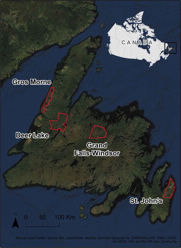
The study area encompasses the entire island of Newfoundland, located on the eastern-most coast of Canada (Figure 1). Within its 108,860 km² area is a highly diverse landscape, characterized by a range of geology, vegetation, and climate. Temperatures on the island in the summer average around 16°C and 0°C in the winter, though these averages will vary locally, ranging between 12°C to 17°C in summer and as low as −3.5°C in winter (Government of Newfoundland and Labrador 2008). Average annual precipitation across the island falls around 1300 mm, but again may range as high as 1600 mm or more and as low as 1200 m (Government of Newfoundland and Labrador 2008). As such, various land cover typifies the Newfoundland landscape, including dense boreal forest, rolling heath, and sprawling peatlands. The current anthropogenic land cover makes up roughly 11% of the island’s total area, with the largest concentration in and amongst the capital city of St. John’s and a number of smaller cities and communities, including Corner Brook, Gander, Grand Falls-Windsor, and Deer Lake.

Figure 1. The Island of Newfoundland and the locations of the study areas within which field data was collected

Wetlands are a dominant feature of the Newfoundland landscape, making up an estimated 18% of the total land cover, the majority of which are peatlands, including bog and fen (National Wetlands Working Group 1997). While there has been extensive work dedicated to establishing the current extent of wetlands across the island (Mahdianpari et al. 2018; Mohammadimanesh et al. 2018a), there exists very little information as it regards to past and future trends of wetland loss and change. Estimates state that around 80–98% of wetlands in and around Canadian cities and two-thirds of coastal marsh in Atlantic Canada have been lost since the time of settlement (Austen and Hanson 2007; Renzetti and Dupont 2017). However, the specifics of wetland loss and change in Newfoundland are not yet known. Likely causes for historical wetland loss and change on the island include wetland drainage and conversion to urban or agricultural land-use. Similar pressures are likely to drive future trends in wetland loss and change, though climate change is a confounding factor (Edvardsson et al. 2015; von Sengbusch 2015).

The wetland ground-truth data that provided the basis for the multi-year reference dataset used in this research was obtained via field campaigns conducted in summers of 2015, 2016, and 2017, originally carried out for use in a project to develop remote sensing methods for mapping wetlands in Newfoundland and Labrador (Mahdianpari et al. 2017b). This field campaign resulted in a total of 432 wetlands visited. The purpose of these field campaigns were to visit and classify as many wetlands as time and effort would allow, in study areas across the province including St. John’s, Deer Lake, Grand Falls-Windsor, and Gros Morne. Please refer to Figure 1 for the location of these field collection areas within Newfoundland. Because the field campaigns had time and budget constraints, a traditional sampling method was not feasible. Rather, to ensure that as many wetlands were visited as possible, wetlands were selected for ground-truthing on the basis of accessibility (adjacent to road and pathways), prior local knowledge, and the visual analysis of Google Earth imagery.

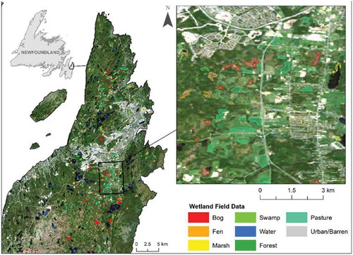
Upon visiting a wetland, a team of ecologists and biologists classified the wetland as bog, fen, swamp, or marsh (described further in Table 1) based on the guidelines provided by the Canadian Wetland Classification System (National Wetlands Working Group 1997). Ultimately 432 wetlands with a size greater than or equal to one hectare were classified and later digitized into polygons, creating a wetland training dataset for the years 2015–2017. To ensure a more accurate classification of wetlands, additional land cover classes, such as urban, pasture, forest, and water (also described in Table 1) were digitized and included in the final dataset. These classes were chosen as they were the most dominant non-wetland land cover classes reported by the Crop Inventory map provided by the Government of Canada through the Department of Agriculture and Agri-foods (Agriculture and Agri-food Canada 2018). Ultimately, the final dataset was comprised of 817 total polygons, 432 of which were wetland and 382 were non-wetland polygons. Figure 2 shows a sample of the digitized ground-truthed polygons in the St. John’s study area.

Table 1. Definitions of wetland and non-wetland classes

Type	Class	Description
Wetland	Bog	Peatland that only receives water via precipitation. Dominated by sphagnum moss, sedges, and ericaceous shrubs.
	Fen	Peatland that receives water from multiple sources. Dominated by brown mosses, sedges, grasses, and shrubs.
	Swamp	Wetland dominated by greater than 30% cover by tall woody trees and/or shrubs often found in association with other hydrological systems.
	Marsh	Wetland with shallow water that fluctuates over time. Dominated by graminoids and other emergent and submerged aquatic plants.
Non-Wetland	Water	Open water areas (ponds, lakes, rivers) with no emergent or floating vegetation.
	Forest	Area of land covered by conifer and deciduous tree canopy.
	Agriculture	Land that is used for the production of crops or for pasture.
	Urban/Barren	Non-vegetated land which includes built-up area or exposed rock.

Figure 2. A snapshot of the reference wetland and non-wetland data collected around the St. John’s study area

The 2015–2017 dataset was used as the basis for the creation of an additional three datasets representing wetland and non-wetland land cover across the island during the years of 1985–87, 1995–97, and 2005–07. To do this, each of the 817 polygons from the 2015–2017 dataset were compared with historical reports, 50 cm aerial photos, and Landsat imagery of the relevant dates to find areas where the polygons in the dataset did not reflect the land cover of the time period. Polygons were modified or removed where any past land cover changes had occurred. For example, a polygon representing urban land cover in 2015–17 did not represent urban land cover in 1985–87 due to the conversion of forest to built-up between these time periods. Similarly, the extent of marsh wetland polygons changes between years due to differences in levels of precipitation between days, seasons, or years. As such, changes to polygons were made within each time period to reflect these differences.

2.2. Data collection and pre-processing

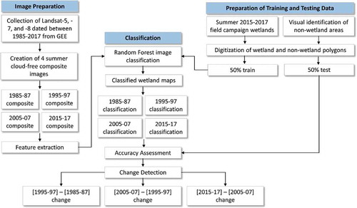
A general summary of our methods including can be seen in Figure 3.

Figure 3. General methodology flowchart used in the study

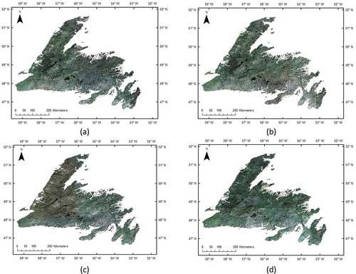
In our study, surface reflectance Tier 1 data products of three different Landsat images (Landsat 5, 7 and 8) from 1985 to 2017 were obtained from the GEE Data Catalog (a public domain resource). Table 2 summarizes the specifications of the data used in this study. These sensors have a 15° field of view and their data scene size is approximately 185 km × 180 km (Arvidson et al. 2006; Roy et al. 2014). Although the Landsat archive contains remotely sensed imagery, which was continuously acquired since 1972, frequent cloud cover results in excessive temporal gaps in the Landsat data for certain regions, especially in wetland areas or during specific time periods. In order to achieve the study objectives and prepare cloud-free composites, each composite was created using the minimal cloud cover and overlapped images of three consecutive years [1985–1987, 1995–1997, 2005–2007, 2015–2017] taken from June 1 to October 30. Finally, four composites made up of 284 images, including 135 Thematic Mapper (TM), 50 Enhanced Thematic Mapper Plus (ETM+), and 99 Operational Land Imager/Thermal Infrared Sensor (OLI/TIRS) with almost free cloud cover were prepared and contain the median reflectance values of the collections The Landsat composites can be seen in Figure 4. Notably, since 2003, due to failure of the scan-line corrector (SLC) of ETM+ imager on Landsat 7, approximately 22% of the pixels of ETM+ images have no data (Wu et al. 2020).

Table 2. The number of Landsat imagery and cloud cover threshold employed in each composite

Composite	Period	Landsat satellite	Number of Images	Cloud cover
First	1985–1987	Landsat 5 TM	62	<20%
Second	1995–1997	Landsat 5 TM	46	<10%
Third	2005–2007	Landsat 7 ETM+ Landsat 5 TM	50 + 27	<15%
Fourth	2015–2017	Landsat 8 OLI/TIRS	99	<20%

Figure 4. The Landsat composites for (a) 1985–87, (b) 1995–97, (c) 2005–07, and (d) 2015–17

A common way to fill no data stripes is utilizing SLC-off gaps filling method (Chen et al. 2011), but in this case, some of the stripes may not get filled due to the cloud cover threshold employed in each composite. To deal with this problem, the third image composite was created by using both Landsat 5 and Landsat 7 images. Note that the similar bands of different Landsat sensor types (TM, ETM+ or OLI/TIRS), including Blue, Green, Red, NIR, shortwave infrared 1(SWIR1), shortwave infrared 2 (SWIR2) and thermal infrared (TIR) bands, were chosen and stacked to create composites. Additionally, to improve the classification results, different spectral indices were calculated and added to the composites. To maintain consistency we did not involve panchromatic bands of Landsat 7 and 8 in composites due to the lack of panchromatic band in Landsat 5 data series.

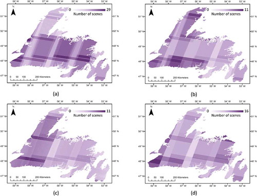
A number of common vegetation indices were calculated, though only the following were included based on variable importance analysis (discussed later): the difference vegetation index (DVI), NDVI, generalized difference vegetation index (GDVI), green normalized difference vegetation index (GNDVI), green-red vegetation index (GRVI), green soil-adjusted vegetation index (GSAVI), green-optimized soil-adjusted index (GOSAVI), soil-adjusted vegetation index (SAVI), optimized soil-adjusted index (OSAVI), enhanced vegetation index (EVI), normalized difference water index (NDWI), TasselledCap Wetness (TCW), and TasselledCap Vegetation (TCV). Additionally, these composites contain one band consisting of the Shuttle Radar Topography Mission (SRTM) V4 digital elevation for providing elevation data of the study site. Please see Table 3 for the index formulae. The selected bands and indices were used as input features for the classification. Figure 5 illustrates the number of Landsat observations over the summer of the aforementioned years.

Table 3. Vegetation Index Formulae

No.	Abbrev.	Formula
1	DVI	2.4NIR−Red
2	NDVI	$\frac{\mathrm{N}\mathrm{I}\mathrm{R}-\mathrm{R}\mathrm{e}\mathrm{d}}{\mathrm{N}\mathrm{I}\mathrm{R}+\mathrm{R}\mathrm{e}\mathrm{d}}$$\frac{\mathrm{N}\mathrm{I}\mathrm{R}-\mathrm{R}\mathrm{e}\mathrm{d}}{\mathrm{N}\mathrm{I}\mathrm{R}+\mathrm{R}\mathrm{e}\mathrm{d}}$
3	GDVI	$\mathrm{N}\mathrm{I}\mathrm{R}-\mathrm{G}\mathrm{r}\mathrm{e}\mathrm{e}\mathrm{n}$$\mathrm{N}\mathrm{I}\mathrm{R}-\mathrm{G}\mathrm{r}\mathrm{e}\mathrm{e}\mathrm{n}$
4	GNDVI	$\frac{\mathrm{N}\mathrm{I}\mathrm{R}-\mathrm{G}\mathrm{r}\mathrm{e}\mathrm{e}\mathrm{n}}{\mathrm{N}\mathrm{I}\mathrm{R}+\mathrm{G}\mathrm{r}\mathrm{e}\mathrm{e}\mathrm{n}}$$\frac{\mathrm{N}\mathrm{I}\mathrm{R}-\mathrm{G}\mathrm{r}\mathrm{e}\mathrm{e}\mathrm{n}}{\mathrm{N}\mathrm{I}\mathrm{R}+\mathrm{G}\mathrm{r}\mathrm{e}\mathrm{e}\mathrm{n}}$
5	GRVI	$\frac{\mathrm{N}\mathrm{I}\mathrm{R}}{\mathrm{G}\mathrm{r}\mathrm{e}\mathrm{e}\mathrm{n}}$$\frac{\mathrm{N}\mathrm{I}\mathrm{R}}{\mathrm{G}\mathrm{r}\mathrm{e}\mathrm{e}\mathrm{n}}$
6	SAVI	$\frac{\mathrm{N}\mathrm{I}\mathrm{R}-\mathrm{R}\mathrm{e}\mathrm{d}}{\mathrm{N}\mathrm{I}\mathrm{R}+\mathrm{R}\mathrm{e}\mathrm{d}+0.5}\times 1.5$$\frac{\mathrm{N}\mathrm{I}\mathrm{R}-\mathrm{R}\mathrm{e}\mathrm{d}}{\mathrm{N}\mathrm{I}\mathrm{R}+\mathrm{R}\mathrm{e}\mathrm{d}+0.5}\times 1.5$
7	GSAVI	$\frac{\mathrm{N}\mathrm{I}\mathrm{R}-\mathrm{G}\mathrm{r}\mathrm{e}\mathrm{e}\mathrm{n}}{\mathrm{N}\mathrm{I}\mathrm{R}+\mathrm{G}\mathrm{r}\mathrm{e}\mathrm{e}\mathrm{n}+0.5}\times 1.5$$\frac{\mathrm{N}\mathrm{I}\mathrm{R}-\mathrm{G}\mathrm{r}\mathrm{e}\mathrm{e}\mathrm{n}}{\mathrm{N}\mathrm{I}\mathrm{R}+\mathrm{G}\mathrm{r}\mathrm{e}\mathrm{e}\mathrm{n}+0.5}\times 1.5$
8	OSAVI	$\frac{\mathrm{N}\mathrm{I}\mathrm{R}-\mathrm{R}\mathrm{e}\mathrm{d}}{\mathrm{N}\mathrm{I}\mathrm{R}+\mathrm{R}\mathrm{e}\mathrm{d}+0.16}$$\frac{\mathrm{N}\mathrm{I}\mathrm{R}-\mathrm{R}\mathrm{e}\mathrm{d}}{\mathrm{N}\mathrm{I}\mathrm{R}+\mathrm{R}\mathrm{e}\mathrm{d}+0.16}$
9	GOSAVI	$\frac{\mathrm{N}\mathrm{I}\mathrm{R}-\mathrm{G}\mathrm{r}\mathrm{e}\mathrm{e}\mathrm{n}}{\mathrm{N}\mathrm{I}\mathrm{R}+\mathrm{G}\mathrm{r}\mathrm{e}\mathrm{e}\mathrm{n}+0.16}$$\frac{\mathrm{N}\mathrm{I}\mathrm{R}-\mathrm{G}\mathrm{r}\mathrm{e}\mathrm{e}\mathrm{n}}{\mathrm{N}\mathrm{I}\mathrm{R}+\mathrm{G}\mathrm{r}\mathrm{e}\mathrm{e}\mathrm{n}+0.16}$
10	EVI	$2.5\times \frac{\mathrm{N}\mathrm{I}\mathrm{R}-\mathrm{R}\mathrm{e}\mathrm{d}}{\left(\mathrm{N}\mathrm{I}\mathrm{R}+6\mathrm{R}\mathrm{e}\mathrm{d}-7.5\mathrm{B}\mathrm{l}\mathrm{u}\mathrm{e}\right)+1}$$2.5\times \frac{\mathrm{N}\mathrm{I}\mathrm{R}-\mathrm{R}\mathrm{e}\mathrm{d}}{\left(\mathrm{N}\mathrm{I}\mathrm{R}+6\mathrm{R}\mathrm{e}\mathrm{d}-7.5\mathrm{B}\mathrm{l}\mathrm{u}\mathrm{e}\right)+1}$
11	NDWI	$\frac{\mathrm{S}\mathrm{W}\mathrm{I}\mathrm{R}1-\mathrm{N}\mathrm{I}\mathrm{R}}{\mathrm{S}\mathrm{W}\mathrm{I}\mathrm{R}1+\mathrm{N}\mathrm{I}\mathrm{R}}$$\frac{\mathrm{S}\mathrm{W}\mathrm{I}\mathrm{R}1-\mathrm{N}\mathrm{I}\mathrm{R}}{\mathrm{S}\mathrm{W}\mathrm{I}\mathrm{R}1+\mathrm{N}\mathrm{I}\mathrm{R}}$
12	TCW	$\left(\mathrm{a}\right)\mathrm{B}\mathrm{l}\mathrm{u}\mathrm{e}+\left(\mathrm{b}\right)\mathrm{G}\mathrm{r}\mathrm{e}\mathrm{e}\mathrm{n}+\left(\mathrm{c}\right)\mathrm{R}\mathrm{e}\mathrm{d}+\left(\mathrm{d}\right)\mathrm{N}\mathrm{I}\mathrm{R}-\left(\mathrm{e}\right)\mathrm{S}\mathrm{W}\mathrm{I}\mathrm{R}1-\left(\mathrm{f}\right)\mathrm{S}\mathrm{W}\mathrm{I}\mathrm{R}2$$\left(\mathrm{a}\right)\mathrm{B}\mathrm{l}\mathrm{u}\mathrm{e}+\left(\mathrm{b}\right)\mathrm{G}\mathrm{r}\mathrm{e}\mathrm{e}\mathrm{n}+\left(\mathrm{c}\right)\mathrm{R}\mathrm{e}\mathrm{d}+\left(\mathrm{d}\right)\mathrm{N}\mathrm{I}\mathrm{R}-\left(\mathrm{e}\right)\mathrm{S}\mathrm{W}\mathrm{I}\mathrm{R}1-\left(\mathrm{f}\right)\mathrm{S}\mathrm{W}\mathrm{I}\mathrm{R}2$
13	TCV	$\left(\mathrm{a}\right)\mathrm{B}\mathrm{l}\mathrm{u}\mathrm{e}-\left(\mathrm{b}\right)\mathrm{G}\mathrm{r}\mathrm{e}\mathrm{e}\mathrm{n}-\left(\mathrm{c}\right)\mathrm{R}\mathrm{e}\mathrm{d}+\left(\mathrm{d}\right)\mathrm{N}\mathrm{I}\mathrm{R}+\left(\mathrm{e}\right)\mathrm{S}\mathrm{W}\mathrm{I}\mathrm{R}1-\left(\mathrm{f}\right)\mathrm{S}\mathrm{W}\mathrm{I}\mathrm{R}2$$\left(\mathrm{a}\right)\mathrm{B}\mathrm{l}\mathrm{u}\mathrm{e}-\left(\mathrm{b}\right)\mathrm{G}\mathrm{r}\mathrm{e}\mathrm{e}\mathrm{n}-\left(\mathrm{c}\right)\mathrm{R}\mathrm{e}\mathrm{d}+\left(\mathrm{d}\right)\mathrm{N}\mathrm{I}\mathrm{R}+\left(\mathrm{e}\right)\mathrm{S}\mathrm{W}\mathrm{I}\mathrm{R}1-\left(\mathrm{f}\right)\mathrm{S}\mathrm{W}\mathrm{I}\mathrm{R}2$

Figure 5. Distribution and number of Landsat scenes in (a) 1985–87, (b) 1995–97, (c) 2005–07, and (d) 2015–17 image composites used in this study

2.3. Post-classification change detection

Using GEE, a pixel-based classification of multi-temporal composites was produced to assess change regions and produce change detection maps. The available classification algorithms within GEE include Classification and Regression Tree (CART), minimum distance (MD) decision tree (DT), random forest (RF), support vector machine (SVM), etc. The RF (Breiman 2001) model is a well-known ensemble classifier that effectively distinguishes between spectrally similar land covers. The robustness of this algorithm has been proven in the literature (de Sousa et al. 2020). RF is also particularly beneficial in wetland classification studies, as this algorithm does not assume normality of training data. This is valuable given that many ground-truthed wetland datasets do not have a normal distribution due to nonrandom methods used in the field as a result of budget, time, and other feasibility constraints.

There are a number of tuning parameters available for RF implementation, including the fraction of the input to bag per tree (bagFraction), the number of decision trees to create per class (Ntree), the number of variables per split (Mtry), and the minimum size of a terminal node (Belgiu and Drăguţ 2016; Goldblatt et al. 2016). For the purposes of this study, the optimum values for these parameters were selected via trial and error. The final parameter values used for this work are listed in Table 4, with a bagFraction parameter of 0.5, an Ntree value of 150, and an Mtry value equal to the square root of the number of total variables as is the best choice according to the literature (Belgiu and Drăguţ 2016; Gislason, Benediktsson, and Sveinsson 2006).

Table 4. The optimal values for the tuning parameters for the RF classifier

Parameter Name	Parameter Value
Number of decision trees	150
Number of variables in each node split	5
Minimum size of a terminal node	2
Fraction of the input to bag per tree	0.5
Number of random seeds	5

RF also allows for the estimation of the importance of a large number of predictor variables included in the classification model. This feature of RF is useful for multi-source data set studies, where data dimensionality is high. As such, it is important to know how each predictive feature influences the classification model and consequently the change detection scheme to be able to select the best variables and to optimize feature space (Rodriguez-Galiano et al. 2012; (Corcoran, Knight, and Gallant 2013); Belgiu and Drăguţ 2016). GEE uses the GINI index as the default split rule, which then propagates into importance. GINI is one of the two RF methods (the other is Mean Decrease in Accuracy) to estimate the importance of each predictor variable.

For purposes of comparison, and to demonstrate the effectiveness of RF for wetland classification as highlighted in the literature, classification was conducted using CART and MD methods in addition to RF. Once the classification models were applied to the composites of each time period, pixel-by-pixel comparison of classified maps generated the change maps.

2.4. Validation and accuracy assessment

To assess the accuracy of the CART, MD, and RF classifications, a portion of the training field-collected dataset was conserved for validation, also refered to as the testing dataset. Because supervised classifiers, such as RF and CART use pre-labeled samples to train the classifier model and are sensitive to imbalanced training data sets, the strategies used for providing the training and testing sampling data must be carefully considered (Ramezan, Warner, and Maxwell 2019; Stehman and Czaplewski 1998). There are a variety of sampling methods in the literature, such as simple random sampling, systematic sampling and stratified sampling, and all have been applied to split training and testing samples for RS applications (Wang et al. 2012).

However, the main problem with the random sampling methods is the information leak between the training and validation dataset (e.g., pixels from same polygon are selected on both training and validation dataset). As such, in this study, a polygon-sampling unit has been adopted and, based on the following procedure, we split the ground truth data into 50% of training and 50% test samples. For each class, reference polygons were first sorted by size and alternatingly assigned to testing and training categorizes. Due to the wide variation of size within each wetland class (some small, some large), random assignment of reference samples to testing and training groups could result in these groups having highly uneven pixel counts. However, alternative assignment ensures that both the testing and the training groups had comparable pixel counts for each class.

To provide error analysis and assessment of classified maps, and consequently, the change detection results, overall accuracy (OA) rate, Kappa Coefficient, F1-Score, user’s accuracy (UA) and producer’s accuracy (PA) were estimated based on confusion matrices. These metrics are widely used for accuracy and quality assessment of remote sensing products, such as change detection, classification, target detection, etc. (Jafarzadeh and Hasanlou 2019; Kelley, Pitcher, and Bacon 2018).

3. Results

Figure 6 shows the distribution of land cover classes across Newfoundland for each time-period, and Figure 7 shows the total coverage of each land cover class as estimated from the final classifications. Based on these results, bog and forest are consistently the most dominant wetland and non-wetland land in Newfoundland for all years, respectively. Marsh is consistently the least common wetland class, having the lowest coverage of any wetland class during all periods. Agriculture and urban/barren are the least common land cover classes overall. These results are as expected as the majority of the Newfoundland landscape has not been altered by human modifications.

Figure 6. Wetland and non-wetland land cover classification using Landsat imagery from 1985–87 (top left), 1995–97 (top right), 2005–07 (bottom left) and 2015–17 (bottom right)

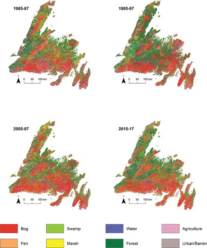
Figure 7. The total area of each wetland and non-wetland land cover class per period of time

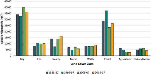
Bog wetland coverage is the lowest during the earliest years studied (1985–87 and 1995–97), and highest in the most recent (2005–07 and 2015–17). The fen and swamp results reflect this trend somewhat, with fen having the lowest coverage in 1985–87 and swamp in 1995–97. The total amount of the marsh class, however, seems to alternate between years, being highest in 1985–87 and 2005–07 and lowest in 1995–97 and 2015–17. Bog coverage is far more extensive than all other wetland classes during every time period. Swamp is the second most extensive wetland class for all periods except 1995–97, during which fen is more extensive.

The result of the accuracy assessment of the RF, CART, and MD classified maps are shown in Tables 5, 6, and 7, respectively.

Table 5. Accuracy assessment of classified maps based on RF method

Composite	Estimator	Bog	Fen	Swamp	Marsh	Water	Forest	Pasture	Urban
1985–87	PA UA OA Kappa F1-Score	91.13	49.29	26.67	48.0	98.29	92.90	87.75	96.52
		82.44	56.45	54.55	85.71	98.29	82.20	95.55	96.52
		84.66
		0.81
		0.77
1995–97	PA UA OA Kappa F1-Score	96.30	61.53	28.57	40.0	90.9	100	85.71	88.23
		76.47	80.0	66.67	66.67	100	85.29	85.71	100
		84.48
		0.81
		0.78
2005–07	PA UA OA Kappa F1-Score	97.30	32.35	20.0	54.54	100	96.87	92.30	92.5
		75.0	61.12	33.34	60.0	96.67	95.38	100	94.87
		84.37
		0.80
		0.75
2015–17	PA UA OA Kappa F1-Score	100	57.89	42.85	50.0	100	100	94.44	100
		80.95	91.67	100	100	100	88.63	100	90.0
		88.96
		0.86
		0.86

Table 6. Accuracy assessment of classified maps based on CART method

Composite	Estimator	Bog	Fen	Swamp	Marsh	Water	Forest	Pasture	Urban
1985–87	PA UA OA Kappa F1-Score	81.82	40.90	50.0	60.0	100	91.66	94.45	93.87
		79.74	40.90	71.42	75.0	100	88.0	77.27	95.83
		82.84
		0.79
		0.77
1995–97	PA UA OA Kappa F1-Score	92.0	42.10	20.0	40.0	100	86.04	100	91.67
		81.17	47.05	66.67	80.0	94.11	88.05	92.0	89.19
		83.87
		0.80
		0.75
2005–07	PA UA OA Kappa F1-Score	91.78	35.0	18.75	28.57	97.72	89.23	90.0	97.29
		70.52	56.0	33.34	36.37	100	86.56	94.73	90.0
		78.64
		0.74
		0.72
2015–17	PA UA OA Kappa F1-Score	84.32	50.57	45.28	44.82	100	94.14	97.61	91.07
		79.6	50.0	55.81	61.90	98.50	93.65	97.61	90.26
		82.7
		0.79
		0.78

Of the classification results, MD method produced the lowest UA and PA (Table 7). While the RF method generally produced the highest UA and PA scores (Table 5), CART produced better results for these parameters in a small number of cases (Table 6, as exemplified 1985–87 swamp wetlands where the RF UA and PA was 26.67 and 54.55, respectively, while CART UA and PA were 50.0 and 71.42, respectively. The MD method also produced the lowest F1-score at 0.40. Though the CART method produced scores close to that of RF, the RF method produced the highest F1-scores. Ultimately, the MD method produced the lowest OA scores and the RF method produced the highest, where the 2015–17 classification had the highest OA at about 89%, followed by the 2005–2007 classification at 85%, the 1985–87 classification at 84% and the 1995–97 classification at 83%.

Table 7. Accuracy Assessment of classified maps based on Minimum Distance method

Composite	Estimator	Bog	Fen	Swamp	Marsh	Water	Forest	Pasture	Urban
1985–87	PA UA OA Kappa F1-Score	0	0	0	46.15	100	0	0	0
		0	0	0	5.17	29.21	0	0	0
		13.39
		0.05
		0.12
1995–97	PA UA OA Kappa F1-Score	25.48	27.08	13.63	11.42	100	48.93	65.21	30.65
		58.24	33.76	8.10	4.45	50.64	66.34	19.86	97.67
		39.31
		0.32
		0.41
2005–07	PA UA OA Kappa F1-Score	37.4	25.0	42.85	8.34	100	53.42	42.85	21.62
		47.27	38.46	20.0	4.17	51.47	78.0	26.47	72.73
		44.96
		0.35
		0.42
2015–17	PA UA OA Kappa F1-Score	17.15	20.48	36.84	16.67	100	46.67	54.92	8.69
		60.34	23.28	24.56	4.08	34.05	75.49	18.48	100
		32.53
		0.24
		0.40

For the RF classification results, generally, across all time periods non-wetland land-use had the highest user and producer accuracies between 91% and 100%. Of the wetland classes, bog had the overall highest producer’s accuracies between 92% and 97%, and fen had the highest user’s accuracies between 66% and 86%. Marsh generally had higher user and producers accuracy values compared to that of the swamp, which had the lowest accuracy results of all classes, wetland and non-wetland.

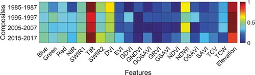
The RF method is not only useful for making prediction but also for assessing the importance of each variable in the classification scheme. The variable importance analysis is a bi-product of RF classification and determines the contribution of each predictor variable to the general classification model. Figure 8 lists the importance of the RF variables applied in this study. Figure 9 illustrates the normalized importance variable of extracted features in this study. As shown, the TIR band and SRTM elevation data were the essential features for wetland classification in different years, followed by NDWI and DVI indices. It is interesting to see that the same features play approximately the same role in the classification of different composites.

Figure 8. Result of RF variable importance to find a ranking of important variables

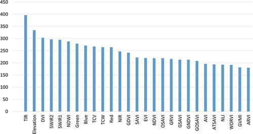
Figure 9. A heat map of efficiency of selected variables based on the RF variable importance measure in classification of different image composites

Figure 10(a,b), and c show the total amount of wetland coverage lost and gained between 1985–87 and 1995–97, between 1995–97 and 2005–07, and between 2005–07 and 2015–17, respectively. Overall, the time-period between 1985–87 and 1995–97 was the only time during which there was a net loss of wetlands as a single class. The results also show a net gain of wetlands as a single class between 1995–97 and 2005–07, and between 2005–07 and 2015–17.

Figure 10. Loss and gain of wetland class land coverage between (a) 1985–97 to 1995/97, (b) 1995–97 to 2005–07, and (c) 2005–07 to 2015–17

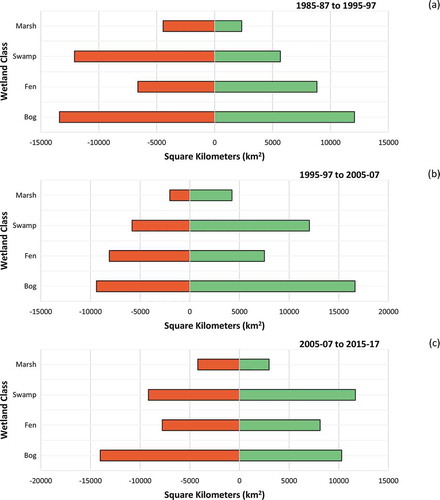
Between 1985–87 and 1995–97 (Figure 10(a–c)), all wetland classes except for fen experienced a net loss in coverage, with swamp experiencing the most significant decrease. Much of the swamp loss during this time period appears to be a result of conversion into forest areas. Similarly, the loss of bog is mostly a result of conversion to fen. Between 1995–97 and 2005–07, fen coverage experienced a small net loss while bog, swamp and marsh experienced a net gain, respectively. The gain in swamp brought its total area back to a similar level, as was present in 1985–87. Between 2005–07 and 2015–17, bog and marsh experienced a net loss, while swamp experienced a net gain. Fen also experienced a small net gain.

Figure 11 shows the total amount of wetland coverage lost due to conversion to anthropogenic land cover, including agriculture and urban (Figure 11(a)), other wetland classes (Figure 11(b)), and non-wetland natural land cover, including forest and water (Figure 11(c)). Generally, the most significant contributor to the loss within an individual wetland class seems to be the conversion to another wetland class, particularly in the case of bog and fen. Bog, for example, is often lost because of conversion to the fen class and vice versa, though a substantial amount of bog and fen has also converted to upland forest. Based on the results in Figure 11(b), the loss within a wetland class because of a conversion to another class is most prominent between 2005–07 and 2015–17. While a large portion of swamp and marsh loss seems to be a result of wetland class conversion, an even more substantial portion is driven by conversion to non-anthropogenic upland classes such as forest and open water (Figure 11(c)). A greater amount of total marsh and swamp area is lost to the conversion to non-anthropogenic upland than bog or fen.

Figure 11. (a) conversion of wetlands to anthropogenic land cover including urban and agriculture, (b) conversion of one wetland class to another, and (c) conversion of wetlands to forest or water land cover

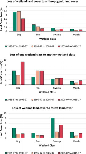
Conversion of wetlands to non-anthropogenic upland is most prominent between 1985–87 and 1995–97, and least prominent between 1995–97 and 2005–07. Compared to other categories of land cover (wetland and non-anthropogenic upland), the conversion of wetlands to anthropogenic classes is less common (Figure 11(a)). The most considerable loss of wetlands to anthropogenic land cover seems to have occurred between 1985–87 and 1995–97. The lowest amount of bog and fen conversion to anthropogenic land cover occurred most recently, between 2005–07 and 2015–17. Conversely, loss of swamp and marsh to anthropogenic land cover seems to have increased slightly during this time period.

Table 8 and Figure 12 provide information regarding the amount and location of wetlands that remained stable or unstable across time periods. Stable wetland areas are those wetland classes that remained the same class across time. Unstable wetlands areas are areas of land that: (1) were classified as wetland during an earlier time period, but became non-wetland in more recent time periods (2) were classified as non- wetland during an earlier period, but became wetland in more recent times or, (3) changed wetland class over time (i.e. an area classed as bog in 1985–87 was classed as fen in 2007–05).

Table 8. Area of wetland class that has changed and area of wetland class that remained unchanged between time periods

	1985–87 to 1995–97		1995–97 to 2005–07		2005–07 to 2015–17
Wetland Class	Unchanged  (km^2)	Changed (km^2)	Unchanged (km^2)	Changed (km^2)	Unchanged (km^2)	Changed (km^2)
Bog	20,683	25,465	23,350	26,039	25,966	24,309
Fen	1558	15,463	2284	15,623	2022	15,898
Swamp	1838	17,774	1697	17,858	4568	20,839
Marsh	2471	6784	2791	6264	2840	7179
Total	26,550	65,486	30,122	65,784	35,396	68,225

Figure 12. Areas where a wetland class remained unchanged over time (green), and areas that were or became a wetland (purple) between 1985–87 to 1995–97, 1995–97 to 2005–07 and 2006–07 to 2015–17

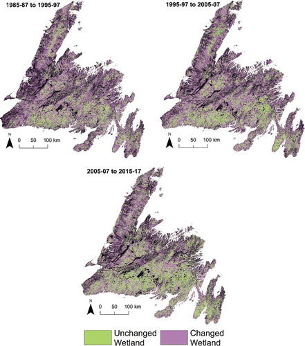
Generally, a majority of areas experienced wetland instability compared to wetland stability (Table 8). This is also the case for individual wetland classes. For example, for all time periods, the area of stable swamp is less than areas of unstable swamp presence. All time periods experienced greater instability and less stability, at similar rates. Specifically, there is 38, 936 km² (42%) more unstable wetland area than the stable area between 1985–87 and 1995–97, 35, 662 km² (37%) more unstable wetland area than the stable area between 1995–97 and 2005–07, and 32, 829 km² (32%) more unstable wetland area versus stable area between 2005–07 and 2015–17. Note, however, that instability seems to decrease slightly as time progresses.

4. Discussion

Though there has been extensive work recently dedicated to the mapping and classification of Newfoundland’s wetlands (Mahdianpari et al. 2017b, 2018; Mohammadimanesh et al. 2018d) there has been little information regarding rates of wetland loss and gain over time. This information is pertinent for informing on the effectiveness of government policies and for assessing the potential impacts of climate change, changing local populations and industry. Additionally, assessing changes to coverage of wetland classes allows for an indirect assessment of the loss and gain of valuable wetland services, many of which are tied directly to wetland class (Hanson 2008; Mohammadimanesh et al. 2018b). The results of this work help to elucidate various trends in wetland change over 30 years on the island of Newfoundland, explicitly reporting on gains and loss of specific wetland classes, including bog, fen, swamp and marsh. While work on the wetland change detection has already been conducted across China (Cao et al. 2020), the US (Ballanti et al. 2017; Fickas, Cohen, and Yang 2016) and Canada (Wulder et al. 2018), none thus far have been conducted in Newfoundland, nor at the scale of the wetland class.

In this study, an RF classifier was employed due to its efficiency and high potential for mapping wetlands’ land cover (Mahdianpari et al. 2020b, 2020a). The RF classification approach presents several advantages in the remote sensing of wetlands when compared with other image classification methods, as demonstrated via the comparison with CART and MD methods. RF is beneficial because it is non-parametric, an efficient tool in processing large, high classification accuracy, continuous and categorical data sets, not sensitive to noise or overtraining, capable of providing ancillary information such as classification error and variable importance, and computationally lighter than other tree ensemble methods (Belgiu and Drăguţ 2016; Rodriguez-Galiano et al. 2012).

Based on the results of this work, several patterns of interest have arisen. For example, the major cause for wetland class loss across Newfoundland is the conversion from one wetland class to another, or conversion to a non-anthropogenic upland class (see Figure 11(b,c)). The conversion of one wetland class to another is sometimes a natural part of a wetlands succession, as is exemplified by the conversion of fen to bog (Tiner 2017). However, accelerated or substantial rates of class conversion may also be a result of climate change, or a result of anthropogenic modifications to the landscape (Pasquet, Pellerin, and Poulin 2015; von Sengbusch 2015). Peatlands such as bog and fen, for example, may experience drying as a result of increased temperatures, decreased precipitation, and modified water flow and water tables (Breeuwer et al. 2009; Potvin et al. 2015). This drying will, in turn, allow for the establishment of woody vegetation over time, resulting in the conversion of bog or fen to swamp.

Similarly, the injection of excess nutrients into a bog, via pollution in the air or run-off, may result in a shift in vegetation from bog-like to fen-like (Hedwall, Brunet, and Rydin 2017; Nishimura and Tsuyuzaki 2015). Notably, much of the loss of bog and fen wetland coverage in Newfoundland is attributed to the conversion to swamp or upland forest, or the conversion of bog and fen alternatively. Similarly, the results show that the loss of marsh and swamp wetlands is primarily due to conversion to open water and forest, respectively. This also may be due in part to climate change, where-by a warming climate, for example, may cause some swamps to dry, becoming more similar in vegetation composition to the upland forest.

While climate change is likely a contributing factor to such changes in wetlands across Newfoundland, additional confounding factors should be considered when interpreting these results. For one, separating swamp from the upland forest has always been a difficult challenge, mainly when using lower resolutions (Jahncke et al. 2018). Thus, there is potential for some misclassification between swamp and forest amongst several years examined in this research, causing a misrepresentative amount of swamp loss to forest and vice versa. This problem is commonly solved by adding Synthetic Aperture Radar (SAR) data to the classification methodology. SAR imagery with longer wavelengths, such as ALOS imagery, is recommended. This is because SAR signals with longer wavelengths can penetrate through vegetation canopy, capturing the structure below and thus providing more information for allowing for the discrimination between the swamp and upland forest (Adeli et al. 2020). Unfortunately, SAR data does not have the historical database that Landsat does, and thus, cannot be used in long-term change detection studies.

Similarly, much marsh vegetation is emergent, and its growth is closely related to local weather patterns and the growing season, which may vary from year to year. Additionally, if a satellite image captures a marsh on a particularly wet day, after an excess of rain, for example, a marsh may appear to be flooded entirely with little to no exposed vegetation, resulting in a classification of open water and a recorded loss of marsh wetlands. Confusion between bog and fen classes is also a common problem in wetland classification, as many bog and fen share very similar vegetation patterns (Bourgeau-Chavez et al. 2017; National Wetlands Working Group 1997; Touzi, Deschamps, and Rother 2007). Such information on the dynamics of wetlands and the difficulties associated with their classification must be considered when interpreting change detection of wetland classes, and when drawing any conclusion as to the cause of wetland loss over time, particularly because this work did not check weather patterns on the dates on satellite imagery acquisition. Future work may investigate weather patterns during image acquisition more clearly, in an effort to choose more weather-consistence imagery over time. Inspection of weather conditions for each Landsat scene is feasible; however, this becomes more difficult as the number of images and the extent of study area size increases.

Other limitations of this work which should be considered when interpreting the results include the low spatial resolution of the classification (relative to other free imagery such as Sentinel-2) and the nonrandom collection of field training data (thus introducing spatial bias). It is likely that all of these factors can contribute to the reliability of the wetland classification results, and should be considered in any research moving forward. However, some of these limitations are unavoidable. The lower resolution Landsat data (verses Sentinel-2) is the only freely available dataset with the historical catalog reaching back as far as the 1980’s. Additionally, field data collection for wetlands is often limited by time and budget constraints, and thus, much wetland classification research must work with data obtained using less than ideal field sampling methods.

Related, the results also show a general instability of wetland area across Newfoundland, where wetland instability seems to be concentrated in much of Newfoundland’s central region, and the north and west coasts. As has been discussed, most of this wetland instability seems to be driven by changes to other wetland classes or to other non-anthropogenic natural upland classes, rather than changes due to direct anthropogenic activity. This general dominance of instable verses stable wetland class presence is likely driven by multiple factors. Climate change may be one such factor, where warming temperatures and changes to rates of precipitation may impact hydrology and vegetation leading to apparent changes in wetland class, which have been discussed above. However, climate change is unlikely to be the only cause. Another driver of instability may be a result of differences in local weather patterns during the times when the images were captured, as has been discussed, which may have impacts on the way wetland classes are visualized in the satellite imagery. For example, if an image was captured after a particularly rainy period verses an image taken after a particularly dry period. Such considerations are more difficult when working with such a large area, and such a substantial time period, given the large number of images that must be processed.

While wetlands are reported as being generally unstable, the loss in area of most wetland classes is generally offset by gains of the same class in different, across all time periods, with some exceptions such as the net loss of fen between 1995–97 and 2005–07, and bog and marsh between 2005–07 and 2015–17. While the offset of loss by comparable gains is of benefit in that there is a comparable offset in the overall loss of wetland services, changes in the location of certain wetland classes in the landscape may have negative impacts on the surrounding ecosystems. For example, a loss of marsh in the upper areas of a watershed may have an impact in the quality of water (in terms of nutrients and pollutants) entering downstream ecosystems. Similarly, a loss of bog or fen to another class in a watershed may have impacts on the overall ability of that watershed to store and release water during times of excess or low water availability.

The results of this work represent the first, to our knowledge, large-scale change detection analysis in Canada performed at the level of four wetland classes defined by the Canadian Wetland Classification System (bog, fen, swamp, and marsh), ultimately producing highly accurate results. Assessment of change at the level of class is of importance because each wetland class provides unique ecosystem services that are of great value to humankind (Hanson 2008). Additionally, this work establishes a justification for the assessment of wetland change detection at the level of class across the entirety of Canada’s landscape using the GEE and Landsat imagery over the past 30 years. While there has been work dedicated to assessing wetland change patterns across Canada previously (Wulder et al. 2018) and work toward assessing the current extents of wetland classes across the country (Mahdianpari et al. 2020b), there has yet to be an attempt to assess countrywide change at the level of the wetland class. Information on rates of change to wetland classes may not only help to elucidate impacts of climate change across the country but also allow for a more in-depth assessment of the loss and modification of class-specific wetland services. Such information will also allow for the fair assessment and comparison of various federal and provincial based wetland protection and management policies across Canada.

5. Conclusions

Understanding large-scale wetland dynamics is of great importance in the era of global climate change and information exchange. Knowledge of change to wetlands at the class level is of particular importance due to the class-related services that these wetlands provide, such as improving the lives of humans and non-human animals alike. At the time of realizing this research, there has not yet been an analysis to detect large-scale wetland change at the class level in Canada. As such, the objective of this research was to support the potential of such application by investigating the feasibility and applicability of historical Landsat imagery and GEE cloud-computing platform on a large scale and time basis, over a single province in Canada. In particular, we used available machine learning algorithms in the GEE platform and Landsat surface reflectance data to detect wetland classes and understand wetland land cover dynamics over time.

The results of this study provide for the first time, an assessment of wetland spatial dynamics across the entirety of Newfoundland at the level of the wetland class. The results reveal that bog, fen, swamp, marsh, water, forest, pasture and urban have experienced significant instability over the past 30 years, mostly because of climate change and anthropogenic activities. These results support the further application of these methods to a future change detection study of the entirety of Canada and confirm the usefulness of the archived Landsat images in the GEE for monitoring long-term wetland dynamics over the past three decades. Such information will allow stakeholders to not only compare statistics as it relates to wetland gain and loss but also allow for the comparison of the effectiveness and quality of province-based wetland policies, which in turn may allow for the general improvement of these policies across the country.

As wetlands are susceptible to multiple factors, including climate change, population growth, and land-use conversion, it is necessary to develop effective policies for the process of wetland protection and restoration. Additionally, future methods in particular should consider classification and change detection methods applicable at geographical scales never possible before, using large amounts of data to address this growing geographical coverage. This is particularly relevant given the global scale of climate change and associated impacts, and increasing globalization. Based on the potential of the Landsat data archive and GEE cloud-computing platform, in future work, we plan to apply this methodology to the entire country of Canada and potentially to the US, in hopes of contributing to the expansion of knowledge of as it relates to North American wetlands and wetland conservation.

Disclosure statement

No potential conflict of interest was reported by the authors.

References

- Adeli, S., B. Salehi, M. Mahdianpari, L. J. Quackenbush, B. Brisco, H. Tamiminia, and S. Shaw. 2020. “. Wetland Monitoring Using SAR Data: A Meta-Analysis and Comprehensive Review.” Remote Sensing 12: 2190. doi:10.3390/rs12142190.
- Agriculture and Agri-food Canada. 2018. “ISO 19131 Annual Crop Inventory – Data Product Specifications.” Agriculture and Agri-Food Canada 27: 1–21.
- Arvidson, T., S. Goward, J. Gasch, and D. Williams. 2006. “Landsat-7 Long-Term Acquisition Plan.” Photogrammetric Engineering & Remote Sensing 72: 1137–1146. doi:10.14358/PERS.72.10.1137.
- Austen, E., and A. Hanson. 2007. “An Analysis of Wetland Policy in Atlantic Canada.” Canadian Water Resources Journal 32: 163–178. doi:10.4296/cwrj3203163.
- Ayanlade, A., and U. Proske. 2016. “Assessing Wetland Degradation and Loss of Ecosystem Services in the Niger Delta, Nigeria.” Marine and Freshwater Research 67: 828–836. doi:10.1071/MF15066.
- Ballanti, L., K. Byrd, I. Woo, and C. Ellings. 2017. “Remote Sensing for Wetland Mapping and Historical Change Detection at the Nisqually River Delta.” Sustainability 9: 1919. doi:10.3390/su9111919.
- Belgiu, M., and L. Drăguţ. 2016. “Random Forest in Remote Sensing: A Review of Applications and Future Directions.” ISPRS Journal of Photogrammetry and Remote Sensing 114: 24–31. doi:10.1016/j.isprsjprs.2016.01.011.
- Boucher, D., S. Gauthier, N. Thiffault, W. Marchand, M. Girardin, and M. Urli. 2020. “How Climate Change Might Affect Tree Regeneration following Fire at Northern Latitudes: A Review.” New Forest 51: 543–571. doi:10.1007/s11056-019-09745-6.
- Bourgeau-Chavez, L. L., S. Endres, R. Powell, M. J. Battaglia, B. Benscoter, M. Turetsky, E. S. Kasischke, and E. Banda. 2017. “Mapping Boreal Peatland Ecosystem Types from Multitemporal Radar and Optical Satellite Imagery.” Canadian Journal of Forest Research 47: 545–559. doi:10.1139/cjfr-2016-0192.
- Bovolo, F., and L. Bruzzone. 2006. “A Theoretical Framework for Unsupervised Change Detection Based on Change Vector Analysis in the Polar Domain.” IEEE Transactions on Geoscience and Remote Sensing 45: 218–236. doi:10.1109/TGRS.2006.885408.
- Breeuwer, A., B. J. M. Robroek, J. Limpens, M. M. P. D. Heijmans, M. G. C. Schouten, and F. Berendse. 2009. “Decreased Summer Water Table Depth Affects Peatland Vegetation.” Basic and Applied Ecology 10: 330–339. doi:10.1016/j.baae.2008.05.005.
- Breiman, L. 2001. “Random Forests.” Machine Learning 45: 5–32. doi:10.1023/A:1010933404324.
- Byun, E., S. A. Finkelstein, S. A. Cowling, and P. Badiou. 2018. “Potential Carbon Loss Associated with Post-settlement Wetland Conversion in Southern Ontario, Canada.” Carbon Balance and Management 13: 6. doi:10.1186/s13021-018-0094-4.
- Cao, W., Y. Zhou, R. Li, and X. Li. 2020. “Mapping Changes in Coastlines and Tidal Flats in Developing Islands Using the Full Time Series of Landsat Images.” Remote Sensing of Environment 239: 111665. doi:10.1016/j.rse.2020.111665.
- Chen, J., X. Zhu, J. E. Vogelmann, F. Gao, and S. Jin. 2011. “A Simple and Effective Method for Filling Gaps in Landsat ETM+ SLC-off Images.” Remote Sensing of Environment 115: 1053–1064. doi:10.1016/j.rse.2010.12.010.
- Connor, R. 2015. The United Nations World Water Development Report 2015: Water for a Sustainable World. Paris: UNESCO publishing.
- Corcoran, J. M., J. F. Knight, and A. L. Gallant. 2013. “Influence of Multi-Source and Multi-Temporal Remotely Sensed and Ancillary Data on the Accuracy of Random Forest Classification of Wetlands in Northern Minnesota.” Remote Sensing 5: 3212–3238. doi:10.3390/rs5073212.
- de Sousa, C., L. Fatoyinbo, C. Neigh, F. Boucka, V. Angoue, and T. Larsen. 2020. “Cloud-computing and Machine Learning in Support of Country-level Land Cover and Ecosystem Extent Mapping in Liberia and Gabon.” PloS One 15: e0227438. doi:10.1371/journal.pone.0227438.
- Edvardsson, J., R. Šimanauskienė, J. Taminskas, I. Baužienė, and M. Stoffel. 2015. “Increased Tree Establishment in Lithuanian Peat Bogs — Insights from Field and Remotely Sensed Approaches.” Science of the Total Environment 505: 113–120. doi:10.1016/j.scitotenv.2014.09.078.
- Fang, C., Z. Tao, D. Gao, and H. Wu. 2016. “Wetland Mapping and Wetland Temporal Dynamic Analysis in the Nanjishan Wetland Using Gaofen One Data.” Artificial Neural Network GIS 22: 259–271. doi:10.1080/19475683.2016.1231719.
- Fatikhunnada, A., K. B. Seminar, L. Liyantono, M. Solahudin, and A. Buono. 2018. “Optimization of Parallel K-means for Java Paddy Mapping Using Time-series Satelite Imagery.” TELKOMNIKA Telecommunication Computing Electronics and Control 16: 1409–1415. doi:10.12928/telkomnika.v16i3.6876.
- Fickas, K. C., W. B. Cohen, and Z. Yang. 2016. “Landsat-based Monitoring of Annual Wetland Change in the Willamette Valley of Oregon, USA from 1972 to 2012.” Wetlands Ecology and Management 24: 73–92. doi:10.1007/s11273-015-9452-0.
- Gardner, R. C., S. Barchiesi, C. Beltrame, C. Finlayson, T. Galewski, I. Harrison, M. Paganini, C. Perennou, D. Pritchard, and A. Rosenqvist. 2015. “State of the World’s Wetlands and Their Services to People: A Compilation of Recent Analyses.” SSRN Electronic Journal. doi:10.2139/ssrn.2589447.
- Gibbes, C., J. Southworth, and E. Keys. 2009. “Wetland Conservation: Change and Fragmentation in Trinidad’s Protected Areas.” Geoforum 40: 91–104. doi:10.1016/j.geoforum.2008.05.005.
- Gislason, P. O., J. A. Benediktsson, and J. R. Sveinsson. 2006. “Random Forests for Land Cover Classification.” Pattern Recognition Letters, Pattern Recognition in Remote Sensing (PRRS 2004) 27: 294–300. doi:10.1016/j.patrec.2005.08.011.
- Goldblatt, R., W. You, G. Hanson, and A. K. Khandelwal. 2016. “Detecting the Boundaries of Urban Areas in India: A Dataset for Pixel-based Image Classification in Google Earth Engine.” Remote Sensing 8: 634. doi:10.3390/rs8080634.
- Government of Newfoundland and Labrador. 2008. Newfoundland Ecoregion Brochures. Deer Lake, NL: Department of Environment and Conservation, Parks & Natural Areas Division.
- Hanson, A. R. 2008. Wetland Ecological Functions Assessment: An Overview of Approaches. Ottawa: Canadian Wildlife Service.
- Hedwall, P.-O., J. Brunet, and H. Rydin. 2017. “Peatland Plant Communities under Global Change: Negative Feedback Loops Counteract Shifts in Species Composition.” Ecology 98: 150–161. doi:10.1002/ecy.1627.
- Hu, Y., and Y. Dong. 2018. “An Automatic Approach for Land-change Detection and Land Updates Based on Integrated NDVI Timing Analysis and the CVAPS Method with GEE Support.” ISPRS Journal of Photogrammetry and Remote Sensing 146: 347–359. doi:10.1016/j.isprsjprs.2018.10.008.
- Huang, H., Y. Chen, N. Clinton, J. Wang, X. Wang, C. Liu, P. Gong, J. Yang, Y. Bai, and Y. Zheng. 2017. “Mapping Major Land Cover Dynamics in Beijing Using All Landsat Images in Google Earth Engine.” Remote Sensing of Environment 202: 166–176. doi:10.1016/j.rse.2017.02.021.
- Hussain, M., D. Chen, A. Cheng, H. Wei, and D. Stanley. 2013. “Change Detection from Remotely Sensed Images: From Pixel-based to Object-based Approaches.” ISPRS Journal of Photogrammetry and Remote Sensing 80: 91–106. doi:10.1016/j.isprsjprs.2013.03.006.
- Jafarzadeh, H., and M. Hasanlou. 2019. “An Unsupervised Binary and Multiple Change Detection Approach for Hyperspectral Imagery Based on Spectral Unmixing.” IEEE Journal of Selected Topics in Applied Earth Observations and Remote Sensing 12: 4888–4906. doi:10.1109/JSTARS.2019.2939133.
- Jahncke, R., B. Leblon, P. Bush, and A. LaRocque. 2018. “Mapping Wetlands in Nova Scotia with Multi-beam RADARSAT-2 Polarimetric SAR, Optical Satellite Imagery, and Lidar Data.” International Journal of Applied Earth Observation and Geoinformation 68: 139–156. doi:10.1016/j.jag.2018.01.012.
- Jin, Y., X. Liu, Y. Chen, and X. Liang. 2018. “Land-cover Mapping Using Random Forest Classification and Incorporating NDVI Time-series and Texture: A Case Study of Central Shandong.” International Journal of Remote Sensing 39: 8703–8723. doi:10.1080/01431161.2018.1490976.
- Kaplan, G., and U. Avdan. 2018. “Monthly Analysis of Wetlands Dynamics Using Remote Sensing Data.” ISPRS International Journal of Geo-Information 7: 411. doi:10.3390/ijgi7100411.
- Kelley, L. C., L. Pitcher, and C. Bacon. 2018. “Using Google Earth Engine to Map Complex Shade-grown Coffee Landscapes in Northern Nicaragua.” Remote Sensing 10: 952. doi:10.3390/rs10060952.
- Liu, D., N. Chen, X. Zhang, C. Wang, and W. Du. 2020. “Annual Large-scale Urban Land Mapping Based on Landsat Time Series in Google Earth Engine and OpenStreetMap Data: A Case Study in the Middle Yangtze River Basin.” ISPRS Journal of Photogrammetry and Remote Sensing 159: 337–351. doi:10.1016/j.isprsjprs.2019.11.021.
- Lu, D., P. Mausel, E. Brondízio, and E. Moran. 2004. “Change Detection Techniques.” International Journal of Remote Sensing 25: 2365–2401. doi:10.1080/0143116031000139863.
- Ma, C., G. Y. Zhang, X. C. Zhang, Y. J. Zhao, and H. Y. Li. 2012. “Application of Markov Model in Wetland Change Dynamics in Tianjin Coastal Area, China.” Procedia Environmental Sciences 13: 252–262. doi:10.1016/j.proenv.2012.01.024.
- Mabwoga, S. O., and A. K. Thukral. 2014. “Characterization of Change in the Harike Wetland, a Ramsar Site in India, Using Landsat Satellite Data.” SpringerPlus 3: 576. doi:10.1186/2193-1801-3-576.
- MacDonald, S., and S. J. Birchall. 2019. “Climate Change Resilience in the Canadian Arctic: The Need for Collaboration in the Face of a Changing Landscape.” The Canadian Geographer Le Géographe Canadien cag.12591. doi:10.1111/cag.12591.
- Mahdianpari, M., B. Brisco, J. E. Granger, F. Mohammadimanesh, B. Salehi, S. Banks, S. Homayouni, L. Bourgeau-Chavez, and Q. Weng. 2020a. “The Second Generation Canadian Wetland Inventory Map at 10 Meters Resolution Using Google Earth Engine.” Canadian Journal of Remote Sensing 1–16. doi:10.1080/07038992.2020.1802584.
- Mahdianpari, M., F. Mohammadimanesh, B. Brisco, S. Homayouni, E. R. Gill, E. DeLancey, and L. Bourgeau-Chavez. 2020b. “Big Data for a Big Country: The First Generation of Canadian Wetland Inventory Map at a Spatial Resolution of 10-m Using Sentinel-1 and Sentinel-2 Data on the Google Earth Engine Cloud Computing Platform.” Canadian Journal of Remote Sensing 46: 15–33.
- Mahdianpari, M., B. Salehi, F. Mohammadimanesh, and B. Brisco. 2017a. “An Assessment of Simulated Compact Polarimetric SAR Data for Wetland Classification Using Random Forest Algorithm.” Canadian Journal of Remote Sensing 43: 468–484. doi:10.1080/07038992.2017.1381550.
- Mahdianpari, M., B. Salehi, F. Mohammadimanesh, S. Homayouni, and E. Gill. 2018. “The First Wetland Inventory Map of Newfoundland at a Spatial Resolution of 10 M Using Sentinel-1 and Sentinel-2 Data on the Google Earth Engine Cloud Computing Platform.” Remote Sensing 11: 43. doi:10.3390/rs11010043.
- Mahdianpari, M., B. Salehi, F. Mohammadimanesh, and M. Motagh. 2017b. “Random Forest Wetland Classification Using ALOS-2 L-band, RADARSAT-2 C-band, and TerraSAR-X Imagery.” ISPRS Journal of Photogrammetry and Remote Sensing 130: 13–31. doi:10.1016/j.isprsjprs.2017.05.010.
- McCarthy, M. J., E. J. Merton, and F. E. Muller-Karger. 2015. “Improved Coastal Wetland Mapping Using Very-high 2-meter Spatial Resolution Imagery.” International Journal of Applied Earth Observation and Geoinformation 40: 11–18. doi:10.1016/j.jag.2015.03.011.
- Mitsch, W. J., and J. G. Gosselink. 2000. “The Value of Wetlands: Importance of Scale and Landscape Setting.” Ecological Economics 35: 25–33. doi:10.1016/S0921-8009(00)00165-8.
- Mitsch, W. J., and J. G. Gosselink. 2007. Wetlands. 4th ed. Hoboken, New Jersey: John Wiley & Sons.
- Mohammadimanesh, F., B. Salehi, M. Mahdianpari, B. Brisco, and M. Motagh. 2018a. “Multi-temporal, Multi-frequency, and Multi-polarization Coherence and SAR Backscatter Analysis of Wetlands.” ISPRS Journal of Photogrammetry and Remote Sensing 142: 78–93. doi:10.1016/j.isprsjprs.2018.05.009.
- Mohammadimanesh, F., B. Salehi, M. Mahdianpari, B. Brisco, and M. Motagh. 2018b. “Wetland Water Level Monitoring Using Interferometric Synthetic Aperture Radar (Insar): A Review.” Canadian Journal of Remote Sensing 44: 247–262. doi:10.1080/07038992.2018.1477680.
- Mohammadimanesh, F., B. Salehi, M. Mahdianpari, E. Gill, and M. Molinier. 2019. “A New Fully Convolutional Neural Network for Semantic Segmentation of Polarimetric SAR Imagery in Complex Land Cover Ecosystem.” ISPRS Journal of Photogrammetry and Remote Sensing 151: 223–236. doi:10.1016/j.isprsjprs.2019.03.015.
- Mohammadimanesh, F., B. Salehi, M. Mahdianpari, and M. Motagh, 2018c. “A New Hierarchical Object-Based Classification Algorithm for Wetland Mapping in Newfoundland, Canada, In: IGARSS 2018-2018 IEEE International Geoscience and Remote Sensing Symposium.” Presented at the IGARSS 2018-2018 IEEE International Geoscience and Remote Sensing Symposium, IEEE, Valencia, 9233–9236. doi:10.1109/IGARSS.2018.8517844
- Mohammadimanesh, F., B. Salehi, M. Mahdianpari, M. Motagh, and B. Brisco. 2018d. “An Efficient Feature Optimization for Wetland Mapping by Synergistic Use of SAR Intensity, Interferometry, and Polarimetry Data.” International Journal of Applied Earth Observation and Geoinformation 73: 450–462. doi:10.1016/j.jag.2018.06.005.
- Mutanga, O., and L. Kumar. 2019. “Google Earth Engine Applications.” Remote Sensing 11: 591. doi:10.3390/rs11050591.
- National Wetlands Working Group. 1997. The Canadian Wetland Classification System. Waterloo, Ont: Wetlands Research Branch, University of Waterloo.
- Nielsen, A. A. 2007. “The Regularized Iteratively Reweighted MAD Method for Change Detection in Multi-and Hyperspectral Data.” IEEE Transactions on Image Processing 16: 463–478. doi:10.1109/TIP.2006.888195.
- Nishimura, A., and S. Tsuyuzaki. 2015. “Plant Responses to Nitrogen Fertilization Differ between Post-mined and Original Peatlands.” Folia Geobotanica 50: 107–121. doi:10.1007/s12224-015-9203-2.
- Pasquet, S., S. Pellerin, and M. Poulin. 2015. “Three Decades of Vegetation Changes in Peatlands Isolated in an Agricultural Landscape.” Applied Vegetation Science 18: 220–229. doi:10.1111/avsc.12142.
- Potvin, L. R., E. S. Kane, R. A. Chimner, R. K. Kolka, and E. A. Lilleskov. 2015. “Effects of Water Table Position and Plant Functional Group on Plant Community, Aboveground Production, and Peat Properties in a Peatland Mesocosm Experiment (Peatcosm).” Plant and Soil 387: 277–294. doi:10.1007/s11104-014-2301-8.
- Ramezan, C., T. Warner, and A. Maxwell. 2019. “Evaluation of Sampling and Cross-Validation Tuning Strategies for Regional-Scale Machine Learning Classification.” Remote Sensing 11: 185. doi:10.3390/rs11020185.
- Reiche, J., S. de Bruin, D. Hoekman, J. Verbesselt, and M. Herold. 2015. “A Bayesian Approach to Combine Landsat and ALOS PALSAR Time Series for near Real-Time Deforestation Detection.” Remote Sensing 7: 4973–4996. doi:10.3390/rs70504973.
- Renzetti, S., and D. P. Dupont, Eds. 2017. Water Policy and Governance in Canada, Global Issues in Water Policy. Cham: Springer International Publishing. doi:10.1007/978-3-319-42806-2.
- Rodriguez-Galiano, V. F., B. Ghimire, J. Rogan, M. Chica-Olmo, and J. P. Rigol-Sanchez. 2012. “An Assessment of the Effectiveness of a Random Forest Classifier for Land-cover Classification.” ISPRS Journal of Photogrammetry and Remote Sensing 67: 93–104. doi:10.1016/j.isprsjprs.2011.11.002.
- Roy, D. P., M. A. Wulder, T. R. Loveland, C. E. Woodcock, R. G. Allen, M. C. Anderson, D. Helder, et al. 2014. “Landsat-8: Science and Product Vision for Terrestrial Global Change Research.” Remote Sensing of Environment 145: 154–172. doi:10.1016/j.rse.2014.02.001.
- Sidhu, N., E. Pebesma, and G. Câmara. 2018. “Using Google Earth Engine to Detect Land Cover Change: Singapore as a Use Case.” European Journal of Remote Sensing 51: 486–500. doi:10.1080/22797254.2018.1451782.
- Stehman, S. V., and R. L. Czaplewski. 1998. “Design and Analysis for Thematic Map Accuracy Assessment: Fundamental Principles.” Remote Sensing of Environment 64: 14. doi:10.1016/S0034-4257(98)00010-8.
- Stralberg, D., X. Wang, M.-A. Parisien, F.-N. Robinne, P. Sólymos, C. L. Mahon, S. E. Nielsen, and E. M. Bayne. 2018. “Wildfire-mediated Vegetation Change in Boreal Forests of Alberta, Canada.” Ecosphere 9: e02156. doi:10.1002/ecs2.2156.
- Sulphur, K. C., S. A. Goldsmith, J. M. Galloway, A. Macumber, F. Griffith, G. T. Swindles, R. T. Patterson, H. Falck, and I. D. Clark. 2016. “Holocene Fire Regimes and Treeline Migration Rates in Sub-arctic Canada.” Global and Planetary Change 145: 42–56. doi:10.1016/j.gloplacha.2016.08.003.
- Syphard, A. D., and M. W. Garcia. 2001. “Human-and Beaver-induced Wetland Changes in the Chickahominy River Watershed from 1953 to 1994.” Wetlands 21: 342–353.
- Tamiminia, H., B. Salehi, M. Mahdianpari, L. Quackenbush, S. Adeli, and B. Brisco. 2020. “Google Earth Engine for Geo-big Data Applications: A Meta-analysis and Systematic Review.” ISPRS Journal of Photogrammetry and Remote Sensing 164: 152–170. doi:10.1016/j.isprsjprs.2020.04.001.
- Tiner, R. 2016. Wetland Indicators: A Guide to Wetland Formation, Identification, Delineation, Classification, and Mapping. 2nd ed. Boca Raton, Florida, USA: CRC Press.
- Tiner, R., M. W. Lang, and V. V. Klemas. 2015. Remote Sensing of Wetlands: Applications and Advances. Boca Raton, Florida, USA: CRC press.
- Tiner, R. W. 2017. Wetland Indicators (Second Edition). A Guide to Wetland Formation, Identification, Delineation, Classification, and Mapping. Boca Raton, Florida: CRC Press.
- Touzi, R., A. Deschamps, and G. Rother. 2007. “Wetland Characterization Using Polarimetric RADARSAT-2 Capability.” Canadian Journal of Remote Sensing 33: 12. doi:10.5589/m07-047.
- von Sengbusch, P. 2015. “Enhanced Sensitivity of a Mountain Bog to Climate Change as a Delayed Effect of Road Construction.” Mires and Peat 15: 1–18.
- Wan, L., Y. Xiang, and H. You. 2019. “A Post-Classification Comparison Method for SAR and Optical Images Change Detection.” Geoscience and Remote Sensing Letters 16: 1026–1030. doi:10.1109/LGRS.2019.2892432.
- Wang, J.-F., A. Stein, -B.-B. Gao, and Y. Ge. 2012. “A Review of Spatial Sampling.” SpatStat 2: 1–14. doi:10.1016/j.spasta.2012.08.001.
- Watson, K. B., T. Ricketts, G. Galford, S. Polasky, and J. O’Niel-Dunne. 2016. “Quantifying Flood Mitigation Services: The Economic Value of Otter Creek Wetlands and Floodplains to Middlebury, VT.” Ecological Economics 130: 16–24. doi:10.1016/j.ecolecon.2016.05.015.
- Wu, L., Z. Li, X. Liu, L. Zhu, Y. Tang, B. Zhang, B. Xu, M. Liu, Y. Meng, and B. Liu. 2020. “Multi-Type Forest Change Detection Using BFAST and Monthly Landsat Time Series for Monitoring Spatiotemporal Dynamics of Forests in Subtropical Wetland.” Remote Sensing 12: 341. doi:10.3390/rs12020341.
- Wulder, M. A., Z. Li, E. M. Campbell, J. C. White, G. Hobart, T. Hermosilla, and N. C. Coops. 2018. “A National Assessment ofWetland Status and Trends for Canada’s Forested Ecosystems Using 33 Years of Earth Observation Satellite Data.” Remote Sensing 10: 1623. doi:10.3390/rs10101623.
- Xu, T., B. Weng, D. Yan, K. Wang, X. Li, W. Bi, M. Li, X. Cheng, and Y. Liu. 2019. “Wetlands of International Importance: Status, Threats, and Future Protection.” International Journal of Environmental Research and Public Health 16: 1818. doi:10.3390/ijerph16101818.
- Yan, J., L. Wang, W. Song, Y. Chen, X. Chen, and Z. Deng. 2019. “A Time-series Classification Approach Based on Change Detection for Rapid Land Cover Mapping.” ISPRS Journal of Photogrammetry and Remote Sensing 158: 249–262. doi:10.1016/j.isprsjprs.2019.10.003.
- Zhang, R., C. Tang, S. Ma, H. Yuan, L. Gao, and W. Fan. 2011. “Using Markov Chains to Analyze Changes in Wetland Trends in Arid Yinchuan Plain, China.” Mathematical and Computer Modelling 54: 924–930. doi:10.1016/j.mcm.2010.11.017.
- Zhang, S., X. Na, B. Kong, Z. Wang, H. Jiang, H. Yu, Z. Zhao, X. Li, C. Liu, and P. Dale. 2009. “Identifying Wetland Change in China’s Sanjiang Plain Using Remote Sensing.” Wetlands 29: 302–313. doi:10.1672/08-04.1.
- Zhu, L., X. Liu, L. Wu, Y. Tang, and Y. Meng. 2019. “Long-Term Monitoring of Cropland Change near Dongting Lake, China, Using the LandTrendr Algorithm with Landsat Imagery.” Remote Sensing 11: 1234. doi:10.3390/rs11101234.