Microwave-based vegetation descriptors in the parameterization of water cloud model at L-band for soil moisture retrieval over croplands

ABSTRACT

Synthetic aperture radar (SAR) data have significant potential for soil moisture monitoring because of their high spatial resolution and independence from cloud coverage. However, it is challenging to retrieve soil moisture from SAR data over vegetated areas, as vegetation significantly affects backscattered radar signals. Auxiliary vegetation information obtained from optical images, such as the normalized difference vegetation index (NDVI) and the leaf area index (LAI), is commonly used to correct vegetation effects. However, it is generally difficult to obtain SAR and optical data in the same area simultaneously, because of the discrepancies in satellite coverage and the effects of cloud coverage. This study focuses on whether vegetation descriptors obtained directly from radar data at L-band can adequately parameterize the semi-empirical backscattering water cloud model (WCM) to support soil moisture retrieval. Four vegetation descriptors (three based on radar images and one based on optical images), were chosen to assess the parameterization and calibration of the WCM and the retrieval accuracy of soil moisture. The results showed that the vegetation descriptor of backscattering at VH polarization outperformed the other three vegetation descriptors (NDVI-derived vegetation water content, radar vegetation index, and the ratio of cross-polarization to VV polarization) in the investigation of four crop types (canola, corn, bean, and wheat) based on the Soil Moisture Active Passive Validation Experiment in 2012 (SMAPVEX12) in Canada. For the vegetation descriptor of VH, the overall accuracy of retrieved soil moisture was promising by separating into two growth stages, with unbiased root mean squared errors of 0.056, 0.053, 0.098, and 0.079 cm³/cm³ for canola, corn, bean, and wheat, respectively. The results also confirmed that variations in vegetation growth affect the accuracy of soil moisture retrieval. In addition, the retrieval performance was undermined when the vegetation changed dramatically, leading to variations or uncertainty in the vegetation structure. This study provides new insights into soil moisture retrieval methods with active L-band microwave observations.

KEYWORDS:

• Synthetic aperture radar
• soil moisture
• water cloud model
• Oh model
• vegetation descriptor

1. Introduction

Soil moisture is widely recognized as an important parameter in hydrological, climatological, and agronomical systems (Gherboudj et al. 2011; Finn et al. 2013). The spatial and temporal distribution of soil moisture is especially necessary in agricultural production and irrigation management, as moisture directly affects the growth and development of vegetation (Zhao et al. 2020). Synthetic aperture radar (SAR) data have been widely used in soil moisture retrieval because of their high spatial resolution and penetration ability under almost all weather conditions (Kornelsen and Coulibaly 2013). However, soil moisture variations only incorporate a relatively small portion of contributions into the total backscattering observed by the radar system, compared to soil roughness and vegetation. This makes it difficult to retrieve soil moisture accurately (Kim et al. 2014a).

Soil moisture retrieval has been studied extensively over bare soil, and a variety of models have been established to describe radar backscatter as a function of soil properties, including empirical models (Oh, Sarabandi, and Ulaby 1992; Dubois, van Zyl, and Engman 1995; Oh, Sarabandi, and Ulaby 2002), semi-empirical models (Shi et al. 1997), the numerical model of Maxwell equations in three dimensions (NMM3D; Tsang et al. 2017), physical scattering models (e.g. the integral equation method (IEM; Fung, Li, and Chen 1992), and the advanced IEM (AIEM; Chen et al. 2003)). Therefore, although backscattering from bare soil is well understood, accounting for the roughness effects during soil moisture retrieval is difficult. This normally leads to two unknowns: root-mean-square (RMS) height and correlation length. To reduce the number of unknowns, the correlation length is usually obtained using ancillary data; however, in-situ measurements of this metric are generally difficult to acquire, and their spatial-temporal representativeness is limited (Baghdadi et al. 2002). Various studies have been conducted to avoid a complete reliance on the measured roughness parameters. For instance, Baghdadi et al. (2002, 2004, 2006a) found a strong correlation between the correlation length and RMS height based on IEM and measurement datasets. They replaced the measured correlation length with empirically estimated calibration parameters from experimental databases of radar images and fields. By setting the RMS height to a constant value according to different radar configurations, Lievens et al. (2011a), Lievens and Verhoest (2011b) developed a statistical model to estimate the effective correlation length from backscattering coefficient observations. Some studies have also noted that errors in the RMS height have a greater impact on soil moisture retrieval accuracy, compared with errors in the correlation length (Lievens et al. 2009; Bai, He, and Li 2016). Bai, He, and Li (2016) used a global search method to simultaneously correct the RMS height and correlation length. Davidson et al. (2003) found an approximately linear relationship between RMS height and correlation length over natural soil surfaces. Kim et al. (2012b) found that soil moisture retrieval is not sensitive to the ratio between the correlation length and the RMS height.

Despite the effects of roughness, it is currently highly challenging to determine soil moisture over vegetated areas using SAR data, due to the simultaneous influences of both bare soil and surface vegetation (vegetation height, biomass, and canopy structure) (Dobson and Ulaby 1986; Zribi et al. 2007). The above-mentioned bare soil models cannot be directly applied to vegetated areas because the vegetation canopy itself contains water (Bindlish and Barros 2001), which increases the complexity of electromagnetic scattering (scattering microwave signals and attenuating microwave signals from the soil surface below (Ouellette et al. 2017)). Currently, there are two main types of methods for removing vegetation effects: those based on polarization decomposition and those based on vegetation scattering models. Over the past few decades, various polarization decomposition algorithms have been proposed (Freeman and Durden 1998; Yamaguchi et al. 2005; Hajnsek et al. 2009; Van Zyl, Arii, and Kim 2011; Wang, Magagi, and Goita 2018), most of which are based on fully polarized data. Main vegetation scattering models usually include the water cloud model (WCM; Attema and Ulaby 1978), the Michigan Microwave Canopy Scattering model (Ulaby et al. 1990), the distorted Born approximation (DBA; Lang and Sighu 1983) and the Tor Vergata model (Ferrazzoli and Guerriero 1996). The WCM assumes that the vegetation canopy is a uniform layer of cloud water droplet and ignores the contribution of higher-order scattering (Attema and Ulaby 1978). Only a few parameters are required in the WCM, and its high accuracy in retrieving soil moisture over vegetated areas has ensured its widespread use in backscattering modeling for soil moisture retrieval over vegetated areas (Joseph et al. 2010; Kumar, Hari Prasad, and Arora 2012; He, Xing, and Bai 2014; Liu and Shi 2016).

The selection of vegetation descriptors is an important process when simulating vegetation scattering using the WCM. In previous studies, the contribution of vegetation has mostly been characterized by physiological parameters (e.g. vegetation water content (VWC; Lievens and Verhoest 2011b)), optical vegetation descriptors (e.g. leaf area index (LAI; He, Xing, and Bai 2014) and normalized difference vegetation index (NDVI; Bindlish and Barros 2001)). Being time-consuming, laborious, and costly, vegetation physiological parameter measurements cannot be easily applied in routine operations. Additionally, the use of optical satellite data is usually limited by weather conditions (such as clouds and haze). Moreover, because of differences in satellite coverage capabilities, it is often difficult to obtain both SAR and optical data in the same area simultaneously.

Some researchers have found that cross-polarization (VH or HV) was mainly dominated by volume scattering (Ulaby, Moore, and Fung 1986) and exhibited a strong correlation with the VWC in vegetated areas (Gherboudj et al. 2011). Others have suggested that the radar vegetation index (RVI) (Kim and Van Zyl 2009) and the ratio of VH polarization to VV polarization (Rvhvv) (De Roo et al. 2001) in the L-band had a strong correlation with the VWC. Using microwave-based vegetation descriptors to characterize vegetation in the WCM for soil moisture retrieval is more effective than using vegetation descriptors based on measured vegetation parameters and optical-based vegetation descriptors. However, few studies have investigated this approach to date. As in a previous study (Li and Wang 2018), the use of these descriptors has been evaluated using SAR-derived RVI and VH polarization to calibrate the WCM at C-band based on Radarsat-2 data. Thus, it is necessary to assess the performance of radar-derived vegetation descriptors in backscattering modeling and soil moisture retrieval at L-band, especially considering the future launch of NASA-ISRO SAR (NI-SAR) (Rosen et al. 2016, 2017). Compared with higher frequencies such as C-band, L-band is less sensitive to vegetation, due to its longer wavelength and stronger penetration ability. Therefore, it could obtain more information pertaining to the underlying soil. Meanwhile, the incident angle is normalized to 40º, which provides more insights for future joint retrieval of soil moisture with Soil Moisture Active Passive (SMAP) radiometer data (passive microwave data with incident an angle of 40º at L-band).

To more accurately obtain soil moisture data, various algorithms have been developed to establish a certain relationship between soil moisture and radar backscattering. These include the change detection method (Balenzano et al. 2011), regression analysis method (Bourgeau-Chavez et al. 2013), artificial neural network method (Paloscia et al. 2013), deep learning method (Lee et al. 2018), optimization method (Pierdicca, Pulvirenti, and Bignami 2010), and look-up table retrieval method (Merzouki, McNairn, and Pacheco 2011). In recent years, soil moisture retrieval methods based on multi-temporal (Kim et al. 2014a), multi-incidence angle (Zhu et al. 2019a), and multi-polarization SAR data have also been explored. As the L-band NI-SAR mission (Rosen et al. 2016, 2017) is scheduled to launch in 2022, it is important to develop and validate a robust operational algorithm for implementation at a global scale.

The main purpose of this study is to evaluate the performance of WCM using vegetation descriptors derived from fully polarized L-band microwaves for backscattering modeling and soil moisture retrieval. Here we propose a method to correct the RMS height when calibrating the parameters for the WCM. The soil surface backscattering coefficients were obtained from the calibrated WCM. Then, the soil moisture was obtained using look-up tables, which were built from the Oh2002 model, owing to its relative simplicity and satisfied accuracy (Baghdadi and Zribi 2006b). The performances of the different vegetation descriptors were evaluated against SMAPVEX12/UAVSAR data, CLASIC/PALS data, and in-situ soil moisture observations, providing new insights into algorithm development for present and future satellite missions.

This paper is organized as follows. Section 2 introduces the details of the study area and the data sets. Section 3 presents the calibration of the WCM and the soil moisture retrieval method. The results of calibration and soil moisture retrieval based on different vegetation descriptors are given in Section 4. In Section 5, the discussion focuses on the impact of soil surface roughness parameter selection and vegetation growth changes on the soil moisture retrieval accuracy. The conclusions are then summarized in Section 6. The implementation of this retrieval process can be seen in Figure 2.

2. Materials

2.1. Dataset for method development

2.1.1. Study area

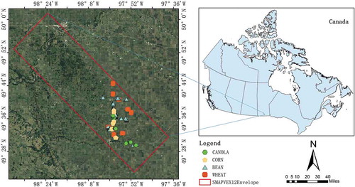
The experimental area of the Soil Moisture Active Passive Validation Experiment 2012 (SMAPVEX12) (Figure 1) is located in the region surrounding southern Manitoba, Canada. Remote sensing and ground measurement data were collected in June and July 2012. The site has an area of 12.8 km × 70 km; its soil texture varies from heavy clay in the east to loamy fine sand in the west. The sudden change in soil texture provides a wide range of soil moisture conditions over a small scale. The landscape of study area features extremely flat terrain, and the typical annual crops are wheat, canola, corn, and beans. In this study, 44 agricultural fields (17 bean fields, 6 corn fields, 15 wheat fields, and 6 canola fields) were selected. Each field covered an area of approximately 50 hectares. Figure 1 shows the geographic locations of the fields in this study.

Figure 1. SMAPVEX12 study area and the location of the ground measurement points for different crops

2.1.2. Remote sensing data

Backscattering coefficient measurements were conducted using uninhabited aerial vehicle synthetic aperture radar (UAVSAR) on different dates (see Table 1). The UAVSAR instrument collected data over a wide range of incidence angles (25° to 65°). The UAVSAR data were normalized to fully utilize the swath, because the incidence angle significantly affected the backscattering coefficients. The SAR instrument was normalized to 40° (the operating angle of the SMAP instrument) through the histogram-based (HIST) technique (Mladenova et al. 2013); this process was performed by Xu (2014) from the Jet Propulsion Laboratory, California Institute of Technology. The processed data were downloaded from the NASA National Snow and Ice Data Center. The L-band (1.26 GHz) data files are provided in a flat binary format on an equiangular grid with a 6 m spatial resolution. Each file contain fully polarimetric SAR data along with an associated XML metadata file. A boxcar filter method (window size 7 × 7) was used to reduce the effects of speckle (Lee and Pottier 2009; Wang, Magagi, and Goita 2017). The NDVI was calculated from SPOT and RapidEye satellite images, and was used to establish an empirical relationship between the measured VWC and NDVI. However, during the SAR observations, only four cloudless optical images were available (see Table 1). The NDVI for other dates were obtained through linear interpolation of these four images. The interpolation of the NDVI between satellite acquisitions caused uncertainty in both the regression with the field observations and the estimation of the VWC value for a specific campaign day. The RMS difference between the VWC obtained by regression and the measured VWC varied between 0.25 and 0.8 kg/m² for different crops (Cosh 2014).

Table 1. Details of the radar and optical data

Data source	Frequency (GHz)	Polarization	Resolution (meters)	Date
SMAPVEX	1.26	Full	6	17/22/25/27/29 June 2012 05/08/10/13/17 July 2012
PALS	1.26	Full	400	11/12/19/23/24/25 June 2007 01/03/04/05/06/7 July 2007
RapidEye	(3.5–6.8)*10^5	-	5	5 July 2012
SPOT-4/5	(1.7–6.8)*10^5	-	5	23/28 June and 5/14 July 2012

2.1.3. Ground measurements

Near-surface (0–6 cm) soil moisture data were collected using hand-held soil moisture probes in each cropland field, during the transit time of the uninhabited aerial vehicles. In addition to soil moisture, surface and subsurface soil temperatures and surface vegetation temperatures were also measured. Sixteen points were sampled in each cropland field, in two rows of eight points. The distance between two points in each row was 75 m and the distance between rows was 200 m. The measurements from the hand-held probes were calibrated by collecting one bulk density core per field (Seyfried et al. 2005; Cosh et al. 2005). The measured volumetric water content of the core was determined using its measured bulk density. After removing the outliers, linear regression was conducted between the core volumetric soil moisture values and the volumetric water content, which was calculated from the dielectric constant obtained by the probe. In order to reduce the uncertainty of in-situ soil moisture measurements, separate calibration equations were developed for each of the 55 fields. The average RMSE value when applying individual calibration equations for each field was 0.037 cm³/cm³ (McNairn et al. 2015). Further details on calibrating the hand-held probe measurements using core volume soil moisture values have been reported by Rowlandson et al. (2013).The volumetric soil moisture values ranged from 0.02 cm³/cm³ to 0.55 cm³/cm³.

For each field, roughness was measured at two sites using a portable pin profilometer. A 1-m profilometer was used to work continuously in one direction to measure the roughness of the long profile (McNairn et al. 2015). Surface displacement and post-processing techniques were used to obtain the RMS height and correlation length.

Vegetation data were collected at 3 of the 16 soil moisture sampling points (sites 2, 11, and 14). At each site, samples were collected to determine that height and stem diameter of the crop. The LAI was measured using hemispherical digital photos (Demarez et al. 2008). The vegetation biomass and the measured VWC were determined by destructive sampling. All data can be downloaded from the National Snow and Ice Data Center website.

2.2. Supplementary dataset for validation

The Cloud and Land Surface Interaction Campaign (CLASIC) experiment was conducted in Oklahoma, USA, from 11 June to 7 July 2007. A fundamental objective of this experiment was to understand the interaction between the atmosphere and the land surface (Jackson et al. 2008). In the experiment, the airborne Passive-Active L-Band System (PALS) was used for ground microwave observations. The PALS flew over the Little Washita (LW) and Fort Cobb (FC) watersheds in Oklahoma for a total of 12 days in 1 month (see Table 1). Each of these watersheds was monitored by the USDA in-situ network, which was used to record soil moisture and weather data (Jackson et al. 2008). During the experiment, 27 fields with an approximate size of 800 m × 800 m (15 in LW and 12 in FC) were sampled to determine soil moisture and related variables. Among them, wheat was planted in 20 fields (10 in LW and 10 in FC). As this study focused on the retrieval of soil moisture in crop areas, wheat fields were selected as verification areas. Extreme rainfall occurred during the experiment, which resulted in waterlogging in the wheat fields. Therefore, the entire experimental area was tested under very humid conditions (Bindlish et al. 2009). The soil moisture retrieval algorithm could only be verified under moderate to very humid conditions.

3. Methodologies

3.1. Radar backscattering models

3.1.1. Rough soil surface

The Oh1992 model defines the co-polarization ratio (p) and cross-polarization ratio (q) of the backscattering coefficients as functions of the soil dielectric constant, soil surface roughness, radar wave number, and incidence angle (Oh, Sarabandi, and Ulaby 1992). D’Urso and Minacapilli (2006) calibrated the Oh1992 model to retrieve soil moisture from bare soil without using prior soil surface roughness data. Wang, Magagi, and Goita (2018) used a two-component polarimetric decomposition method combined with the Oh1992 model to retrieve soil moisture under vegetation cover. Oh, Sarabandi, and Ulaby (2002) constructed the Oh2002 model by considering the influence of correlation length based on the Oh1992 model and improved the calculation of the cross-polarized backscattering coefficients. The Oh2002 model established an empirical relationship between soil moisture and backscattering coefficients; thus, the dielectric constant model was no longer required for conversion between the soil dielectric constant and soil moisture. Concurrently, the Oh2002 model simulates the co-polarized backscattering coefficients more accurately compared with the previous model (Baghdadi and Zribi 2006b). Therefore, the Oh2002 model was used to simulate the backscattering coefficients of the bare soil surface in this study; the formulas are as follows:

(1) ${\sigma }_{VH}^o=0.11{m_v}^{0.7}{\left(cos\theta \right)}^{2.2}\left(1-\mathrm{e}\mathrm{x}\mathrm{p}\left(-0.32{\left(ks\right)}^{1.8}\right)\right)$(1)

(2) $\mathrm{q}=\frac{{\sigma }_{VH}^o}{{\sigma }_{VV}^o}=0.1{\left(\frac{s}{l}+sin\left(1.3\theta \right)\right)}^{1.2}\left(1-\mathrm{e}\mathrm{x}\mathrm{p}\left(-0.9{\left(ks\right)}^{0.8}\right)\right)$(2)

(3) $\mathrm{p}=\frac{{\sigma }_{HH}^o}{{\sigma }_{VV}^o}=1-{\left(\frac{\theta }{{90}^o}\right)}^{0.35{m_v}^{-0.65}}\mathrm{e}\mathrm{x}\mathrm{p}\left(-0.4{\left(ks\right)}^{1.4}\right)$(3)

where θ is the angle of incidence (°), $m_v$is the volumetric soil moisture (cm³/cm³); s is the RMS height (cm); l is the correlation length (cm); k is the radar wave number; and ${\sigma }_{VV}^o$, ${\sigma }_{HH}^o$, and ${\sigma }_{VH}^o$ represent the backscattering coefficients (intensity, m²/m²) of the VV, HH, and VH polarizations, respectively.

In this study, f was taken to be 1.26 GHz and θ was normalized to 40°. The polarization mode was VV. The RMS height was calibrated using a cost function, which is described in detail in Section 3.2, and the correlation length was 10 times the RMS height (Kim et al. 2014a).

3.1.2. Vegetated surface

The backscattering coefficients obtained from the vegetation coverage area can be expressed as follows (Attema and Ulaby 1978):

(4) ${\sigma }_{PP}^o={\sigma }_{veg}^o+{\gamma }^2{\sigma }_{soil}^o$(4)

where ${\sigma }_{PP}^o$ represents the normalized radar cross-section, or the backscattering coefficients of the vegetation coverage area, which consists of two parts. The parameter ${\sigma }_{soil}^o$ is the backscattering coefficient of the soil surface under vegetation, ${\gamma }^2$ is the attenuation coefficient of the vegetation canopy, and ${\sigma }_{veg}^o$ is the direct scattering coefficient of the vegetation canopy. As a low-order approximation, multiple scattering between the vegetation canopy and the soil surface was ignored (Ouellette et al. 2017).

When the vegetation status of adjacent images changes, ${\sigma }_{veg}^o$ and ${\gamma }^2$will change. Therefore, before retrieving soil moisture, it was necessary to eliminate these two effects of vegetation through the WCM. The variables in Equation (5)(5) ${\gamma }^2=\mathrm{e}\mathrm{x}\mathrm{p}\left(-2B{m}_{veg}sec\theta \right)$(5) can be expressed as:

(5) ${\gamma }^2=\mathrm{e}\mathrm{x}\mathrm{p}\left(-2B{m}_{veg}sec\theta \right)$(5)

(6) ${\sigma }_{veg}^o=A{m}_{veg}cos\theta \left(1-{\gamma }^2\right)$(6)

where $m_{veg}$ represents the vegetation parameters of the direct vegetation attenuation and scattering of the canopy. The coefficients A and B are determined by the vegetation canopy type and sensor configuration (Bai et al. 2017), and can be solved using the backscattering coefficients simulated from the WCM and the backscattering coefficients from UAVSAR.

3.1.3. Vegetation descriptors

In the WCM, vegetation parameters are needed to describe the scattering of the vegetation itself and the attenuation of the soil scattered by the vegetation canopy. In this study, four vegetation descriptors (vwc-NDVI, RVI, the ratio between the VH polarization and VV polarization, and the backscattering coefficient of VH polarization) were used to describe the vegetation canopy. The vwc-NDVI is the VWC calculated by establishing a relationship between the measured VWC and NDVI obtained from optical images. More calculation details can be found on the NASA National Snow and Ice Data Center website. RVI is derived from radar observations. It describes the structural characteristics of the crop and is highly correlated with biomass, LAI, and VWC (Kim et al. 2012 2014b); it is not affected by the cloud layer. Rvhvv is the ratio of cross-polarization to VV polarization. Some scholars have found that Rvhvv has a strong correlation with VWC (De Roo et al. 2001; Gherboudj et al. 2011). The final descriptor is the backscattering coefficient of the VH polarized channel. The formulae used to calculate the vegetation descriptors are shown in Table 2.

Table 2. Formulas used to calculate the vegetation descriptors. ${\sigma }_{VV}^o$ and ${\sigma }_{HH}^o$ are the backscattering coefficients of the VV and HH polarizations, respectively, and ${\sigma }_{HV}^o$ is the average backscattering coefficient of the HV and VH polarizations

Vegetation Descriptors	Formula
vwc-NDVI	$\mathrm{V}\mathrm{W}\mathrm{C}=\mathrm{a}\ast \mathrm{N}\mathrm{D}\mathrm{V}\mathrm{I}+\mathrm{b}$ or $\mathrm{V}\mathrm{W}\mathrm{C}=\mathrm{c}\ast \mathrm{e}\mathrm{x}\mathrm{p}\left(\mathrm{d}\ast \mathrm{N}\mathrm{D}\mathrm{V}\mathrm{I}\right)$
RVI	$\mathrm{R}\mathrm{V}\mathrm{I}=\frac{8{\sigma }_{HV}^o}{2{\sigma }_{HV}^o+{\sigma }_{HH}^o+{\sigma }_{VV}^o}$
Rvhvv	$Rvhvv=\frac{{\sigma }_{HV}^o}{{\sigma }_{VV}^o}$
VH	-

3.2. Parameterization and calibration

Calibrating the WCM is essential for developing a retrieval method for soil moisture. This includes obtaining parameters A and B in the WCM, and the RMS height and correlation length in the Oh2002 model. The main steps for WCM calibration are shown in Figure 2 (Calibration part):

Figure 2. Flowchart for the WCM parameterization and soil moisture retrieval

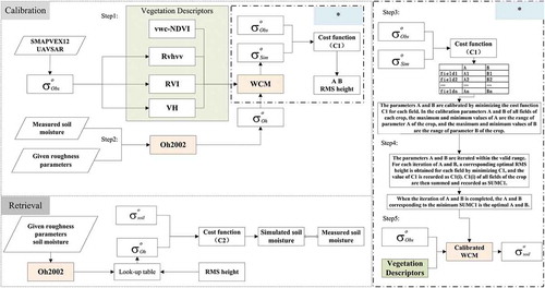
Step 1: Calculation of vegetation descriptors. In addition to the VWC data as a reference target, we also used the pre-processed backscattering coefficients to calculate RVI, Rvhvv and VH as vegetation descriptors.

Step 2: Generating the simulation dataset of backscattering coefficients from the bare soil. The RMS height ranged from 0.1 to 3 cm with an interval of 0.1 cm, and the correlation length was 10 times the RMS height. Note that each field was assumed to have the same roughness condition; however, the roughness between fields was different. Then, the backscattering coefficient of bare soil at VV polarization was simulated by the Oh2002 model according to the airborne radar configuration and the measured soil moisture.

Step 3: Obtaining the valid range of parameters A and B of the WCM for each crop type. The cost function C1 was constructed to minimize the difference between the simulated backscattering coefficients and the observed backscattering coefficients from the SAR image. Parameters A and B were calibrated for each field by minimizing the cost function C1. Then, according to the crop type of each field, the valid ranges of parameters A and B were obtained for each crop type. The cost function was calculated as follows:

(7) $\mathrm{C}1=\sqrt{\frac{1}{n}\sum _{i=1}^n{\left({\sigma }_{Sim\left(i\right)}^o-{\sigma }_{Obs\left(i\right)}^o\right)}^2}$(7)

where ${\sigma }_{Sim}^o$ denotes the simulated radar backscattering coefficient, ${\sigma }_{Obs}^o$ denotes the observed backscattering coefficient from the SAR image, and i and nrepresent the index and number of the data samples.

Step 4: Determining the optimal parameters A and B for each crop type. Parameters A and B are related to crop types. Different fields of the same crop type will have the same values for parameters A and B. For each field of each crop type, parameters A and B were iterated within the valid range. The minimum C1 value for each field of the crop type in question was recorded as C1(i). The C1(i) values of all fields of this crop were then summed and recorded as SUMC1. When the iteration was completed, the values of A and B corresponding to the minimum SUMC1 were taken to be the optimal A and B. In the iterative process, the optimal RMS heights corresponding to each field were obtained concurrently.

Step 5: Calculation of the bare soil backscattering coefficient using the WCM. After obtaining the optimal A and B parameters, the WCM was used to correct the effects of vegetation on the backscattering coefficient and obtain the backscattering coefficient of bare soil. The vegetation descriptors used in the WCM were vwc-NDVI, RVI, Rvhvv, and VH.

3.3. Soil moisture retrieval

Considering the simple principle and highly efficient calculation of the look-up table retrieval method, we used the Oh2002 model to establish a look-up table and used the cost functions to retrieve soil moisture (Figure 2 Retrieval). The soil moisture was retrieved using the corrected optimal roughness parameters (RMS height and correlation length) and the coupled model. The differences in ${\sigma }_{soil}^o$ and${\sigma }_{OH}^o$ at VV polarization were minimized by the cost function C2 to obtain the soil moisture:

(8) $\mathrm{C}2=\sqrt{{\left({\sigma }_{soil}^o-{\sigma }_{OH}^o\right)}^2}$(8)

(9) ${\sigma }_{soil}^o=\frac{{\sigma }_{Obs}^o-{\sigma }_{veg}^o}{{\gamma }^2}$(9)

where ${\sigma }_{soil}^o$ indicates the bare soil backscattering coefficient calculated by the WCM, ${\sigma }_{OH}^o$ indicates the backscattering coefficient from the look-up table, ${\sigma }_{veg}^o$ indicates the direct scattering coefficient of the vegetation canopy, ${\gamma }^2$ indicates the attenuation of vegetation on surface scattering coefficient, and ${\sigma }_{Obs}^o$ indicates the observed backscattering coefficient from the SAR. images.

4. Results

4.1. Sensitivity of vegetation descriptors to VWC

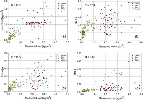
Radar signals are sensitive to the water content of vegetation, which contributes to their attenuation. They are also sensitive to the vegetation structure, which mainly affects the multiple scattering. The VWC is typically used to quantify the effects of vegetation on the radar backscattering process. In this study, we compared the four vegetation descriptors with the measured VWC. Figure 3 shows scatterplots between the vegetation descriptors and the measured VWC. Table 3 lists the correlation coefficients between the four vegetation descriptors of the different crops and the measured VWC. As shown in Figure 3, relationships between the different vegetation descriptors and measured VWC values differ notably. To be noted, the vwc-NDVI obtained from the optical image was calculated by establishing an empirical relationship between the NDVI and the measured VWC. As the measured VWC were collected on nonflight days, there was a time lag between the three vegetation descriptors obtained from radar images and the measured VWC. Radar vegetation descriptors were selected from adjacent dates before and after the measured VWC to create scatter plots, as shown in Figure 3. Here, vwc-NDVI and Rvhvv were highly correlated with the measured VWC, with correlation coefficients of 0.79 and 0.72, respectively. RVI and VH were slightly less correlated with the measured VWC, with correlation coefficients of 0.63 and 0.62, respectively. As vwc-NDVI was obtained by fitting NDVI to the measured VWC, the nonlinearity of VWC and NDVI was eliminated to a certain extent. Therefore, the correlation coefficient between vwc-NDVI and the measured VWC is highest. Comparing the correlation between the vegetation descriptors among different crops and the measured VWC, corn and bean were slightly higher than canola, and the correlation of wheat was the lowest. However, it should be noted that the analysis here only shows the performance of vegetation descriptors in describing the water content inside the vegetation. Moreover, a higher correlation with VWC does not indicate a better descriptive ability regarding the total effects of vegetation.

Table 3. Correlation coefficient between vegetation descriptors and measured VWC

	vwc-NDVI (Reference)	RVI	Rvhvv	VH(%)
canola	0.41	0.49	0.69	0.34
corn	0.82	0.59	0.64	0.84
bean	0.85	0.62	0.61	0.79
wheat	0.39	0.21	0.26	0.33
average	0.79	0.63	0.72	0.62

Figure 3. Scatterplots between the measured VWC and different vegetation descriptors. Different crop types are marked with scatters of different colors

4.2. Parameter tuning and calibration

The inclusion of HH polarization in the cost function slightly reduced the retrieval accuracy of soil moisture; thus, in the entire analysis, only VV polarization was used. In this study, the optimal roughness and parameters A and B were obtained by minimizing the cost function C1. Table 4 lists the average optimal roughness of different fields and parameters A and B of all crops obtained using different vegetation descriptors. To verify the calibrated WCM, the simulated backscattering coefficient calculated by the WCM (${\sigma }_{Sim}^o$) and the backscattering coefficient obtained from the SAR image (${\sigma }_{Obs}^o$) were compared. The four statistical indicators (Bias, RMSE, ubRMSE and correlation coefficient R) used to compare the backscattering coefficient results are listed in Table 4. Figure 4 shows the scatterplots between ${\sigma }_{Sim}^o$ and ${\sigma }_{Obs}^o$. We used the F-test (joint hypotheses test) and calculated the p-value (probability); further, we plotted the 95% confidence interval and 95% prediction interval in the figure.

Table 4. Model coefficients, optimal roughness, and statistical metrics between the ${\sigma }_{Obs}^o$ and ${\sigma }_{Sim}^o$

Vegetation Descriptors	Crop	Model Coefficients		Optimal Roughness		Statistical Metrics
		A	B	s(cm)	l(cm)	R	Bias(dB)	RMSE(dB)	ubRMSE(dB)
vwc-NDVI	Canola	0.0058	0.040	1.80	18.00	0.718	0.020	1.138	1.138
	Corn	0.100	0.035	1.93	19.30	0.806	0.280	1.649	1.625
	Bean	0.0831	0.035	0.51	5.10	0.731	0.333	1.610	1.575
	Wheat	0.0011	0.055	0.93	9.30	0.844	0.068	1.270	1.268
	Overall	0.048	0.041	1.29	12.93	0.902	0.200	1.458	1.444
RVI	Canola	0.291	0.050	1.20	12.00	0.837	0.071	0.978	0.976
	Corn	0.390	0.090	2.40	24.00	0.731	0.017	1.916	1.916
	Bean	0.210	0.070	0.51	5.10	0.688	0.231	1.729	1.713
	Wheat	0.016	0.280	0.82	8.20	0.865	0.201	1.245	1.229
	Overall	0.227	0.123	1.23	12.33	0.892	0.169	1.543	1.534
Rvhvv	Canola	0.390	0.160	1.30	13.00	0.805	0.094	1.014	1.01
	Corn	2.950	0.170	2.30	23.00	0.751	0.069	1.852	1.851
	Bean	0.380	0.310	0.54	5.40	0.657	0.129	1.748	1.743
	Wheat	0.010	0.830	0.86	8.60	0.864	0	1.237	1.237
	Overall	0.930	0.370	1.25	12.50	0.891	0.077	1.541	1.539
VH	Canola	19.80	1.530	1.17	11.70	0.899	−0.067	0.723	0.719
	Corn	17.500	13.500	1.90	19.00	0.935	0.062	0.985	0.983
	Bean	48.100	32.300	0.46	4.60	0.84	0.349	1.315	1.268
	Wheat	29.500	2.700	0.59	5.90	0.895	−0.055	1.095	1.094
	Overall	28.700	12.500	1.03	10.30	0.942	0.129	1.137	1.130

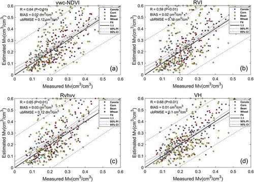
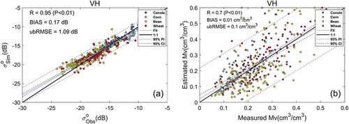
Figure 4. Scatterplots between the ${\sigma }_{Obs}^o$ from radar observations and the ${\sigma }_{Sim}^o$ simulated from the WCM for different vegetation descriptor (a: vwc-NDVI, b: RVI, c: Rvhvv, d: VH). Different crop types are marked with colored dots (canola: blue circles, corn: cyan circles, bean: yellow circles, wheat: red circles). The regressed linear relationship is the solid black line. The 95% confidence interval (CI) is shown by the blue-dashed line, and 95% prediction interval (PI) is shown by the red-dashed line. The statistical metrics in the figure is the total statistical value of the four crops

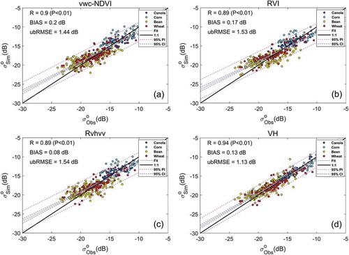
Figure 4 shows that the WCM fitting accuracy based on the VH descriptor was better than that based on the other three vegetation descriptors. The ubRMSE values of the four crops based on the VH descriptor were lower than 1.3 dB at VV polarization. As shown in Table 4, when vwc-NDVI, RVI, and RVHVV were used as vegetation descriptors, canola (corn) has the highest (lowest) fitting accuracy among the four crops. When the VH vegetation descriptor was used instead, canola had the highest fitting accuracy, whereas beans had the lowest fitting accuracy. The fitting accuracies of corn and beans were lower than those of canola and wheat, because the former group of crops were in their growth period, suggesting that their structure changed significantly during the observation period. Moreover, the fitting accuracy values shown in Table 4 differ from the correlation coefficients shown in Table 3, especially for beans and wheat. This indicates that the fitting accuracy of the WCM is related to the VWC, as well as the vegetation type/structure (the fitting accuracy is affected by parameters A and B). Similar conclusions have been reached in other studies when using SMAPVEX12 data. For example, Kim et al. (2012a) found that the soil moisture retrieval results of wheat were better than those of beans. The alpha method was also found to be the most applicable to cereal crops (Ouellette 2015). Soil moisture and vegetation can change simultaneously, which complicates the fitting of the backscattering coefficient.

For the same crop, the obtained optimal roughness varied when different vegetation descriptors were used (Table 4), in agreement with conclusions derived by previous scholars (Bai et al. 2017; Qiu et al. 2019). However, the optimal roughness of each crop was concentrated within a relatively small range. The comparison of the three vegetation descriptors obtained from the radar images shows that the change of surface optimal roughness among various crop types was more significant than those between vegetation descriptors. Notably, the selected optimal roughness parameters had no physical meaning. The parameters were simply used for adjustments to improve the accuracy of soil moisture retrieval, and did not reflect actual surface conditions (Bai, He, and Li 2016). This condition is also the reason for the variations in the ${\sigma }_{Sim}^o$values corresponding to different vegetation descriptors, as shown in Figure 4. ${\sigma }_{Sim}^o$ values were simulated to correspond to the optimal roughness.

4.3. Soil moisture retrieval from different parameterization schemes

The calibrated WCM was used to remove the influence of vegetation and obtain the backscattering coefficients of bare soil. Then, by minimizing the cost function C2, soil moisture was estimated using the backscattering coefficients of bare soil. The Bias, R, RMSE, and ubRMSE values between the estimated soil moisture and the measured soil moisture are listed in Table 5. Figure 5 presents the scatterplots between the measured and estimated soil moisture based on each vegetation descriptor.

Table 5. Statistical metrics between the measured and estimated soil moisture

Vegetation Descriptors	Crop	Statistical Metrics
		R	Bias (cm^3/cm^3)	RMSE (cm^3/cm^3)	ubRMSE (cm^3/cm^3)
vwc-NDVI	Canola	0.670	0.017	0.101	0.099
	Corn	0.517	0.062	0.148	0.134
	Bean	0.552	0.016	0.137	0.137
	Wheat	0.810	0.014	0.088	0.087
	Overall	0.640	0.022	0.120	0.118
RVI	Canola	0.709	0.017	0.108	0.106
	Corn	0.381	0.074	0.168	0.151
	Bean	0.523	0.017	0.153	0.152
	Wheat	0.804	0.005	0.087	0.087
	Overall	0.588	0.022	0.134	0.132
Rvhvv	Canola	0.742	0.011	0.098	0.098
	Corn	0.430	0.061	0.160	0.148
	Bean	0.589	0.027	0.140	0.138
	Wheat	0.811	0.020	0.091	0.089
	Overall	0.646	0.028	0.126	0.123
VH	Canola	0.614	0.011	0.084	0.083
	Corn	0.466	0.038	0.114	0.108
	Bean	0.656	−0.007	0.114	0.113
	Wheat	0.786	0.021	0.088	0.085
	Overall	0.685	0.011	0.103	0.102

Figure 5. Scatterplots between the measured and estimated soil moisture based on each vegetation descriptors. Different crop types are marked with scatters of different colors (canola: blue circles, corn: cyan circles, bean: yellow circles, wheat: red circles). The regressed linear relationship is the solid black line. The 95% confidence interval (CI) is shown by the blue-dashed line, and 95% prediction interval (PI) is shown by the red-dashed line. The statistical metrics in the figure is the total statistical value of the four crops

In general, the statistical metrics of the backscattering coefficients in Table 4 were consistent with the statistical metrics of the soil moisture presented in Table 5. Figure 5 shows that the soil moisture retrieval results using the VH descriptor were more accurate than those obtained using the other three descriptors. When comparing the four crops, regardless of the vegetation descriptor used, the soil moisture retrieval accuracies of corn and beans were lower than those of canola and wheat (Figure 5). For corn, during the observation period of the image, corn was in its growth period, meaning its vegetation structure underwent obvious changes. The low precision of beans was probably caused by its vegetation structure. The results of soil moisture retrieval based on the Rvhvv and vwc-NDVI descriptor were similar, and the accuracy of the retrieval results based on vwc-NDVI was slightly better than those based on Rvhvv (Figure 5). Concurrently, Table 5 shows that for different crops, the range of soil moisture retrieval accuracy varied based on the different vegetation descriptors. The VH descriptor was the most concise of its group, and also produced the highest soil moisture retrieval accuracy. This result is consistent with the findings of Li and Wang (2018), who also used C-band for retrieval.

4.4. Validation with supplementary dataset

To further validate the robustness, the proposed methodology was used to retrieve soil moisture against an independent dataset from CLASIC07. We expected that the tuned vegetation parameters of A and B could be transferred to the same crop type under similar climatic conditions. With the vegetation parameters A and B from the dataset over wheat fields in the SMAPVEX12 experimental areas, only the soil roughness in terms of the RMS height of wheat fields in the CLASIC07 experimental area was obtained through the cost function C1. The wheat plots over the two experimental areas were expected to have a similar structure and, thus, have similar vegetation parameters. The roughness condition, however, was expected to vary from field to field. Similarly, the WCM was used to eliminate the influence of vegetation and obtain the backscattering coefficients from bare soil. Then, the soil moisture was retrieved by minimizing the cost function C2 with the corresponding roughness parameters.

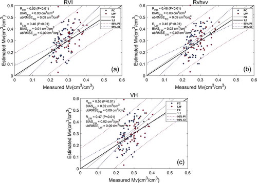
Figure 6 shows the scatterplots between the measured and estimated soil moisture based on different vegetation descriptors for the LW and FC watersheds during the CLASIC07 experiment. It should be noted that only radar-based vegetation descriptors are presented, because of insufficient optical images. The retrieval results of soil moisture based on the different vegetation descriptors in wheat fields showed more similar performances than those from the SMAPVEX12 experimental area. The ubRMSE values were 0.087 cm³/cm³, 0.089 cm³/cm³, and 0.085 cm³/cm³ for RVI, Rvhvv, and VH, respectively, during the SMAPVEX12 experiment. In comparison, the ubRMSE values were 0.091 cm³/cm³, 0.090 cm³/cm³, and 0.093 cm³/cm³ for RVI, Rvhvv, and VH, respectively, during the CLASIC07 experiment. As shown in Figure 6, the correlation coefficient of VH was slightly higher than those of the other microwave-based vegetation descriptors in the CLASIC07 experimental area. The results from the CLASIC07 experiment further confirmed the robustness of the proposed methodology in this study.

Figure 6. The scatterplots between the measured and estimated soil moisture based on each vegetation descriptors for the FC and LW watersheds. Different watersheds are marked with scatters of different colors (FC: blue circles, LW: red circles). The regressed linear relationship is the solid black line. The 95% confidence interval (CI) is shown by the blue-dashed line, and 95% prediction interval (PI) is shown by the red-dashed line. The statistical metrics in the figure is the statistical value of the two watersheds

5. Discussion

5.1. Impacts of crop phenology

Parameters A and B of the WCM were affected by vegetation types and their structures (Bindlish and Barros 2001). When the vegetation changed significantly during the experiment period, the assumption that a set of constant parameters could be used was not valid, and potentially led to failures in both simulation and retrieval. To analyze the influence of vegetation growth changes on the retrieval of soil moisture, this study retrieved the soil moisture in all crop-covered areas across two time periods. The 5-day data in June represent the first growth stage (stem elongation), and the 5-day data in July represent the second growth stage (flowering & fruiting) (Wang, Magagi, and Goita 2016). The observed changes in the vegetation descriptors could reflect changes in vegetation; hence, we analyzed the relationship between the accuracy of soil moisture retrieval and the change of vegetation by calculating the coefficient of variation (CV) of vegetation descriptors (Zhao et al. 2020). Three statistical metrics (standard deviation, average value, and CV) of the vegetation descriptor (VH) are shown in Table 6. Figure 7(a,c) show the scatterplots between${\sigma }_{Obs}^o$and${\sigma }_{Sim}^o$. Figure 7(b,d) show the scatterplots between the measured and estimated soil moisture values; statistical metrics are listed in Table 7. This study mainly analyzed the effectiveness of obtaining vegetation information from radar images; therefore, VH was selected as the vegetation descriptor to analyze the retrieval results of the four crops.

Table 6. Statistical metrics of vegetation descriptor (VH). SD is the standard deviation of the data and MEAN is the average of the data. CV is the coefficient of variation of the data

Growth period	Metrics	canola	corn	bean	wheat
Total growth stage	SD(dB)	−20.774	−20.569	−29.684	−25.597
	MEAN(dB)	−19.119	−20.523	−29.681	−25.297
	CV	0.683	0.989	0.999	0.933
First growth stage	SD(dB)	−20.155	−28.272	−34.433	−28.008
(stem elongation)	MEAN(dB)	−17.786	−26.368	−33.753	−25.382
	CV	0.580	0.645	0.855	0.546
	Second growth stage	canola2	corn2	bean2	wheat2
	SD(dB)	−25.385	−20.915	−29.387	−24.482
	MEAN(dB)	−21.050	−18.118	−27.617	−25.214
(flowering & fruiting)	CV	0.369	0.525	0.665	1.184

Table 7. Statistical metrics between the ${\sigma }_{Obs}^o$ and${\sigma }_{Sim}^o$ and statistical metrics between the measured and estimated soil moisture for two time periods. The first part of the table represents the stem elongation period (Canola1, Corn1, Bean1, and Wheat1), the second part represents the flowering & fruiting period (Canola2, Corn2, Bean2, and Wheat2), and the third part is a summary of the two growth periods (Canola, Corn, Bean, and Wheat)

Vegetation Descriptor	Crop	Statistical Metrics				Soil Moisture Statistical Metrics
		R	Bias (dB)	RMSE (dB)	ubRMSE (dB)	R	Bias (cm^3/cm^3)	RMSE (cm^3/cm^3)	ubRMSE (cm^3/cm^3)
VH	Canola1	0.962	0.043	0.469	0.467	0.778	−0.005	0.064	0.064
	Corn1	0.889	0.078	0.783	0.779	0.884	0.013	0.056	0.055
	Bean1	0.83	0.435	1.419	1.35	0.768	−0.012	0.104	0.103
	Wheat1	0.959	−0.145	0.828	0.815	0.843	0.022	0.078	0.075
	Canola2	0.953	−0.001	0.375	0.375	0.810	0.003	0.046	0.046
	Corn2	0.951	−0.145	0.684	0.668	0.550	0.018	0.053	0.050
	Bean2	0.883	0.183	1.048	1.032	0.650	0.009	0.091	0.091
	Wheat2	0.876	0.067	1.07	1.068	0.680	0.009	0.084	0.084
	Canola	0.967	0.020	0.423	0.423	0.791	−0.001	0.056	0.056
	Corn	0.962	−0.024	0.740	0.740	0.786	0.015	0.055	0.053
	Bean	0.871	0.305	1.242	1.204	0.736	−0.001	0.098	0.098
	Wheat	0.919	−0.028	0.969	0.969	0.795	0.081	0.014	0.079

Figure 7. The scatterplots between ${\sigma }_{Obs}^o$and${\sigma }_{Sim}^o$ and the scatterplots between the measured and estimated soil moisture. (a)(b) is the first growth stage (stem elongation), (c)(d) is the second growth stage (flowering & fruiting). Different crop types are represented by different colors (canola: blue circles, corn: cyan circles, bean: yellow circles, wheat: red circles). The regressed linear relationship is the solid black line. The 95% confidence interval (CI) is shown by the blue-dashed line, and 95% prediction interval (PI) is shown by the red-dashed line

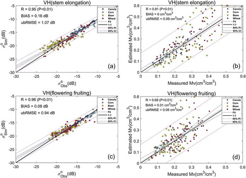
Tables 5 and 6 show that the CV of the VH descriptor throughout the growth period had a close linear relationship with the ubRMSE values of soil moisture retrieval. The correlation coefficient was approximately 0.75. After being divided into two growth stages, the correlation coefficient between the CV of VH and the ubRMSE of soil moisture retrieval was 0.77 in the first growth stage and 0.71 in the second growth stage. A possible explanation for this phenomenon is that the height of vegetation in the second stage was higher than that in the first stage, which may have led to an increase in multiple scattering between the vegetation and the ground (Bindlish et al. 2009). However, the increase in multiple scattering was not completely captured by the VH descriptor; hence, the correlation between the CV of the VH descriptor and the ubRMSE of soil moisture retrieval decreased. Moreover, the variability of the soil moisture can also affect the retrieval accuracy. The effects of the CV of soil moisture on the retrieval accuracy are not discussed in this paper. The calculation formula of CV is as follows:

(10) $\mathrm{C}\mathrm{V}=\frac{SD}{MEAN}$(10)

where SD is the standard deviation of the data and MEAN is the arithmetic mean of the data.

In the first stage, the crops were in the stem elongation period, the plant height accelerated through growth, and the vegetation descriptor changed significantly. In the second stage, during which the crops were in their flowering & fruiting period, the plant height was mostly stable, which decreased the change in the vegetation descriptors. In comparing the retrieval results of different crops, VH was more accurate than the other vegetation descriptors in both periods for canola and beans, and during the flowering & fruiting period of corn. Rvhvv was superior to the other vegetation descriptors in the stem elongation period of corn and wheat. The vwc-NDVI performed best in the flowering & fruiting period of wheat.

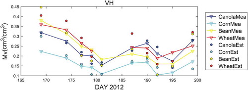
Figure 8 shows the trends of the measured and estimated soil moisture values for each crop. Some points in Figure 8 are missing because of a lack of certain measured soil moisture data. The estimated soil moisture and the measured soil moisture both exhibited similar fluctuations; thus, the changes in soil moisture could be properly captured by the retrieval process (Bai et al. 2017). On the first day, the estimated soil moisture values of the corn and beans were higher than the measured soil moisture values. This was because the fitting parameters of WCM underestimated the vegetation’s contribution to the overall scattering. Figure 8 also shows that the soil moisture retrieval accuracy in the second stage was slightly higher than that in the first stage. For some underestimated points in Figure 8, owing to the change in VWC, the change in soil moisture was not completely captured by the image.

Figure 8. Time series of the measured and estimated soil moisture for each crop. Measured soil moisture are indicated by the lines of different colors. Estimated soil moisture are identified by scatter points of different colors. Lines and dots of the same color represent the same crop (canola: blue circles, corn: cyan circles, bean: yellow circles, wheat: red circles)

5.2. Impacts of soil roughness

In this study, when simulating the backscattering coefficient of bare soil, we assumed that the correlation length was 10 times the RMS height (Kim et al. 2014a). To analyze the common effect of the correlation length and RMS height on the retrieval results, the RMS height and correlation length were corrected simultaneously when simulating the backscattering of bare soil (Bai, He, and Li 2016). As in the previous section 5.1, VH was selected as the vegetation descriptor to analyze the retrieval results of the four crops. Table 8 lists the average optimal roughness for different fields and WCM coefficients. The statistical metrics of ${\sigma }_{Obs}^o$ and${\sigma }_{Sim}^o$ and the statistical metrics of the measured and estimated soil moisture values are also listed in Table 8. Figure 9(a) shows the scatterplots between${\sigma }_{Obs}^o$and${\sigma }_{Sim}^o$, and Figure 9(b) shows the scatterplots between the measured and estimated soil moisture values.

Table 8. Model coefficients, optimal roughness, statistical metrics between the ${\sigma }_{Obs}^o$ and ${\sigma }_{Sim}^o$, and statistical metrics between the measured and estimated soil moisture

	Crop	canola	corn	bean	wheat
Model Coefficients	A	21.1	16.8	47	27.1
	B	1.3	14	31	3.3
Optimal Roughness	s(cm)	1.5	2.1	0.49	0.7
	l(cm)	10.5	16.5	10.4	8.4
Statistical Metrics	R	0.901	0.934	0.865	0.891
	Bias(dB)	−0.011	0.079	0.399	−0.025
	RMSE(dB)	0.709	0.982	1.239	1.11
	ubRMSE(dB)	0.709	0.979	1.173	1.11
Soil Moisture Statistical Metrics	R	0.636	0.472	0.672	0.794
	Bias(cm^3/cm^3)	0.006	0.038	0.013	0.019
	RMSE(cm^3/cm^3)	0.076	0.114	0.108	0.085
	ubRMSE(cm^3/cm^3)	0.076	0.107	0.107	0.083

Figure 9. The scatterplots between the ${\sigma }_{Obs}^o$and${\sigma }_{Sim}^o$(a) and the scatterplots between the measured and estimated soil moisture(b). The statistical metrics in the figure is the total statistical value of the four crops. Different crop types are marked with scatters of different colors (canola: blue circles, corn: cyan circles, bean:yellow circles, wheat: red circles). The regressed linear relationship is the solid black line. The 95% confidence interval (CI) is shown by the blue-dashed line, and 95% prediction interval (PI) is shown by the red-dashed line

A comparison between Tables 4 and 8 reveals that the coefficients of WCM changed slightly under the two roughness correction methods. This result shows that after considering the change of the correlation length, there was little effect on the coefficient of WCM. Compared with Table 4, the RMS height of each crop in Table 8 increased by approximately 0.03–0.33 cm. This discovery indicates that the optimal roughness cannot reflect the actual ground conditions, but is instead a regulation parameter that can improve the soil moisture retrieval accuracy (Bai, He, and Li 2016). The ubRMSE between ${\sigma }_{Obs}^o$and${\sigma }_{Sim}^o$ in Table 8 was similar to that in Table 4, indicating that the concurrent corrections of the correlation length and RMS height approximated the fitting accuracy of the previous correction method. Compared with the statistical metrics of soil moisture presented in Table 5, the soil moisture retrieval accuracy was slightly improved when it was obtained by simultaneously correcting the RMS height and the correlation length. These results indicate that using a correlation length of ten times the RMS height in the experimental area was appropriate (Kim et al. 2014a).

6. Conclusions

This study analyzed the functions of microwave-based vegetation descriptors in the parameterization of WCM and soil moisture retrieval at L-band. The dependence of the WCM on measured vegetation information or optical remote sensing data was overcome; thus, our ability to retrieve soil moisture data was improved. Three vegetation descriptors based on radar images (RVI, Rvhvv, and VH) and one vegetation descriptor based on optical images (vwc-NDVI) were used to parameterize the WCM and evaluate performance regarding backscattering modeling and soil moisture retrieval.

First, compared with the radar observations, the WCM with the VH vegetation descriptor had the best performance, indicating that the VH vegetation descriptor was capable of describing the vegetation effects in both the attenuation and scattering components in the experimental area, under the framework of the WCM. From the data, the ubRMSE value between ${\sigma }_{Obs}^o$ and ${\sigma }_{Sim}^o$ was less than 1.3 dB at VV polarization. Second, parameters A and B of the WCM might change according to vegetation growth, and using a constant value for these parameters throughout crops’ differing growth periods might introduce uncertainty to soil moisture retrieval. For the vegetation descriptor of VH, the overall ubRMSE values of soil moisture retrieval with two separate growing stages (two sets of parameters A and B) were 0.056, 0.053, 0.098, and 0.079 cm³/cm³ for canola, corn, beans, and wheat, respectively. Compared with the results of soil moisture retrieval with one overall growing stage (one set of parameters A and B), the ubRMSE was reduced by approximately 0.01–0.05 cm³/cm³. Finally, our study showed that the roughness effects could be approximated with one parameter, which reduced the total number of unknowns. The soil moisture retrieval accuracy obtained by simultaneously correcting the RMS height and the correlation length was similar to the retrieval results obtained by expressing the correlation length as 10 times the RMS height.

The proposed approach and corresponding model parameters show a certain spatial and temporal transferability through the experimental results of two data sets (the SMAPVEX12 and CLASIC07) with time series observations (Patil and Stieglitz 2015). To evaluate the spatial transferability, the effectiveness of the approach was validated using data from two different research regions (Manitoba, Canada of SMAPVEX12 in 2012 and Oklahoma, USA of CLASIC07 in 2007). The vegetation parameters of A and B obtained from the SMAPVEX12 (Manitoba) dataset were directly used for the soil moisture retrieval from the CLASIC07 (Little Washita and Fort Cobb watersheds in Oklahoma) dataset. Results show that the approach performed well in retrieving soil moisture with the CLASIC07 dataset in Oklahoma, without any recalibration of the model parameters. The soil moisture retrieval accuracy of the two research regions was similar with the ubRMSE (approximately 0.09 cm³/cm³). This shows that the approach and tuned vegetation parameters can be transferred spatially, and can be reused for the same crop type. To evaluate the temporal transferability, the proposed approach in this paper was applied to retrieve soil moisture in two typical periods (first stage of stem elongation, second stage of flowering & fruiting) in the SMAPVEX12 research region. For different crop types, the ubRMSE values ranged between 0.05 and 0.1 cm³/cm³ during the stem elongation period, whereas the ubRMSE values were found to be in the range of 0.04–0.09 cm³/cm³ during the flowering & fruiting period. These results, therefore, suggest that the approach could be transferred from one period to another period. However, our study was only conducted in North America, in areas with humid continental (Manitoba) and the subtropical (Oklahoma) climates. Due to the temporal and spatial variation of crop planting structures, and the complexity of radar interactions between soil and vegetation, the spatial and temporal transferability of the proposed approach needs further verification, and also requires extensive measurements of soil and vegetation properties and corresponding radar observations; these aspects were not addressed in the present study.

These results provide new insights into the parameterization of the WCM and soil moisture retrieval with L-band radar observations, which is of considerable importance in the global mapping of soil moisture with the future development of the NI-SAR mission. It should be noted that this work is based on the assumptions that the soil surface is isotropic and that the soil surface roughness is time-invariant during the research period. Therefore, further verification is needed when this approach is adopted for anisotropic surfaces with periodic structures (Blaes and Defourny 2008), as the surface roughness might vary relative to the radar look direction. Here it was assumed that the surface roughness remains unchanged to reduce the number of parameters to be retrieved. However, the surface roughness could change significantly due to plowing or precipitation, and the experiment period needs to be divided into multiple sections for a better retrieval (Zhu et al. 2019b). In addition, the simple WCM, which ignores the multiple scattering between the soil surface and vegetation, was used to describe the complex radar scattering within the vegetation and soil-vegetation interactions. This might be reasonable for croplands at L-band, but it needs further examination in scenes with more densely-vegetated areas and higher frequencies.

This study was limited only to croplands, with a few cases of crop types. Further studies of more vegetation types, and under different climatic conditions, are needed to verify the robustness of the proposed approach. Notably, L-band radar is less sensitive to vegetation because of its longer wavelength, compared to higher frequencies such as C-band and X-band. Subsequent studies using Sentinel-1 satellite data could be promising in investigating the performance of this approach using C-band, as the Sentinel-1 satellites have a high revisit frequency at a global scale.

Acknowledgements

The authors would like to thank the SMAPVEX12 participants and the NASA National Snow and Ice Data Center for providing the experimental data.

Disclosure statement

No potential conflict of interest was reported by the authors.

Additional information

Funding

This work is supported by the National Key Research and Development Program of China [No.2017YFC0405802] and the National Natural Science Foundation of China [No.41671355, No.41971031, No.41711411].

References

- Attema, E. P. W., and F. T. Ulaby. 1978. “Vegetation Modeled as a Water Cloud.” Radio Science 13 (2): 357–364. doi:10.1029/RS013i002p00357.
- Baghdadi, N., I. Gherboudj, M. Zribi, M. Sahebi, C. King, and F. Bonn. 2004. “Semi-empirical Calibration of the IEM Backscattering Model Using Radar Images and Moisture and Roughness Field Measurements.” International Journal of Remote Sensing 25 (18): 3593–3623. doi:10.1080/01431160310001654392.
- Baghdadi, N., N. Holah, and M. Zribi. 2006a. “Calibration of the Integral Equation Model for SAR Data in C‐band and HH and VV Polarizations.” International Journal of Remote Sensing 27 (4): 805–816. doi:10.1080/01431160500212278.
- Baghdadi, N., C. King, A. Chanzy, and J. P. Wigneron. 2002. “An Empirical Calibration of the Integral Equation Model Based on SAR Data, Soil Moisture and Surface Roughness Measurement over Bare Soils.” International Journal of Remote Sensing 23 (20): 4325–4340. doi:10.1080/01431160110107671.
- Baghdadi, N., and M. Zribi. 2006b. “Evaluation of Radar Backscatter Models IEM, OH and Dubois Using Experimental Observations.” International Journal of Remote Sensing 27 (18): 3831–3852. doi:10.1080/01431160600658123.
- Bai, X., B. He, and X. Li. 2016. “Optimum Surface Roughness to Parameterize Advanced Integral Equation Model for Soil Moisture Retrieval in Prairie Area Using Radarsat-2 Data.” IEEE Transactions on Geoscience and Remote Sensing 54 (4): 2437–2449. doi:10.1109/tgrs.2015.2501372.
- Bai, X., B. He, X. Li, J. Zeng, X. Wang, Z. Wang, Y. Zeng, and Z. Su. 2017. “First Assessment of Sentinel-1A Data for Surface Soil Moisture Estimations Using a Coupled Water Cloud Model and Advanced Integral Equation Model over the Tibetan Plateau.” Remote Sensing 9 (7): 714. doi:10.3390/rs9070714.
- Balenzano, A., F. Mattia, G. Satalino, and M. W. J. Davidson. 2011. “Dense Temporal Series of C- and L-band SAR Data for Soil Moisture Retrieval over Agricultural Crops.” IEEE Journal of Selected Topics in Applied Earth Observations and Remote Sensing 4 (2): 439–450. doi:10.1109/jstars.2010.2052916.
- Bindlish, R., and A. P. Barros. 2001. “Parameterization of Vegetation Backscatter in Radar-based, Soil Moisture Estimation.” Remote Sensing of Environment 76 (1): 130–137. doi:10.1016/s0034-4257(00)00200-5.
- Bindlish, R., T. Jackson, R. Sun, M. Cosh, S. Yueh, and S. Dinardo. 2009. “Combined Passive and Active Microwave Observations of Soil Moisture during CLASIC.” IEEE Geoscience and Remote Sensing Letters 6 (4): 644–648. doi:10.1109/lgrs.2009.2028441.
- Blaes, X., and P. Defourny. 2008. “Characterizing Bidimensional Roughness of Agricultural Soil Surfaces for SAR Modeling.” IEEE Transactions on Geoscience and Remote Sensing 46 (12): 4050–4061. doi:10.1109/tgrs.2008.2002769.
- Bourgeau-Chavez, L. L., B. Leblon, F. Charbonneau, and J. R. Buckley. 2013. “Evaluation of Polarimetric Radarsat-2 SAR Data for Development of Soil Moisture Retrieval Algorithms over a Chronosequence of Black Spruce Boreal Forests.” Remote Sensing of Environment 132: 71–85. doi:10.1016/j.rse.2013.01.006.
- Chen, K. S., T.-D. Wu, L. Tsang, Q. Li, J. Shi, and A. K. Fung. 2003. “Emission of Rough Surfaces Calculated by the Integral Equation Method with Comparison to Three-dimensional Moment Method Simulations.” IEEE Transactions on Geoscience and Remote Sensing 41 (1): 90–101. doi:10.1109/tgrs.2002.807587.
- Cosh, M. 2014. “SMAPVEX12 Vegetation Water Content Map, Version 1.” [Indicate subset used]. Boulder, Colorado USA: NASA National Snow and Ice Data Center Distributed Active Archive Center. doi:10.5067/4C7MN0KJILTI. [Date Accessed].
- Cosh, M. H., T. J. Jackson, R. Bindlish, J. S. Famiglietti, and D. Ryu. 2005. “Calibration of an Impedance Probe for Estimation of Surface Soil Water Content over Large Regions.” Journal of Hydrology 311: 49–58. doi:10.1016/j.jhydrol.2005.01.003.
- D’Urso, G., and M. Minacapilli. 2006. “A Semi-empirical Approach for Surface Soil Water Content Estimation from Radar Data without A-priori Information on Surface Roughness.” Journal of Hydrology 321 (1–4): 297–310. doi:10.1016/j.jhydrol.2005.08.013.
- Davidson, M. W. J., F. Mattia, G. Satalino, N. E. C. Verhoest, T. Le Toan, M. Borgeaud, J. M. B. Louis, and E. Attema. 2003. “Joint Statistical Properties of Rms Height and Correlation Length Derived from Multisite 1-m Roughness Measurements.” IEEE Transactions on Geoscience and Remote Sensing 41 (7): 1651–1658. doi:10.1109/tgrs.2003.813361.
- De Roo, R. D., Y. Du, F. T. Ulaby, and M. C. Dobson. 2001. “A Semi-empirical Backscattering Model at L-band and C-band for A Soybean Canopy with Soil Moisture Inversion.” IEEE Transactions on Geoscience and Remote Sensing 39 (4): 864–872. doi:10.1109/36.917912.
- Demarez, V., S. Duthoit, F. Baret, M. Weiss, and G. Dedieu. 2008. “Estimation of Leaf Area and Clumping Indexes of Crops with Hemispherical Photographs.” Agricultural and Forest Meteorology 148 (4): 644–655. doi:10.1016/j.agrformet.2007.11.015.
- Dobson, M., and F. Ulaby. 1986. “Active Microwave Soil Moisture Research.” IEEE Transactions on Geoscience and Remote Sensing GE-24 (1): 23–36. doi:10.1109/TGRS.1986.289585.
- Dubois, P. C., J. van Zyl, and T. Engman. 1995. “Measuring Soil Moisture with Imaging Radars.” IEEE Transactions on Geoscience and Remote Sensing 33 (4): 915–926. doi:10.1109/36.406677.
- Ferrazzoli, P., and L. Guerriero. 1996. “Emissivity of Vegetation: Theory and Computational Aspects.” Journal of Electromagnetic Waves and Applications 10 (5): 609–628. doi:10.1163/156939396x00559.
- Finn, M. P., M. Lewis, D. D. Bosch, M. Giraldo, K. Yamamoto, D. G. Sullivan, R. Kincaid, R. Luna, G. Allam, and C. Kvien. 2013. “Remote Sensing of Soil Moisture Using Airborne Hyperspectral Data.” GIScience & Remote Sensing 48 (4): 522–540. doi:10.2747/1548-1603.48.4.522.
- Freeman, A., and S. L. Durden. 1998. “A Three-Component Scattering Model for Polarimetric SAR Data.” IEEE Transactions on Geoscience and Remote Sensing 36 (3): 963–973. doi:10.1109/36.673687.
- Fung, A. K., Z. Li, and K. S. Chen. 1992. “Backscattering from a Randomly Rough Dielectric Surface.” IEEE Transactions on Geoscience and Remote Sensing 30 (2): 356–369. doi:10.1109/36.134085.
- Gherboudj, I., R. Magagi, A. A. Berg, and B. Toth. 2011. “Soil Moisture Retrieval over Agricultural Fields from Multi-polarized and Multi-angular RADARSAT-2 SAR Data.” Remote Sensing of Environment 115 (1): 33–43. doi:10.1016/j.rse.2010.07.011.
- Hajnsek, I., T. Jagdhuber, H. Schon, and K. P. Papathanassiou. 2009. “Potential of Estimating Soil Moisture under Vegetation Cover by Means of PolSAR.” IEEE Transactions on Geoscience and Remote Sensing 47 (2): 442–454. doi:10.1109/tgrs.2008.2009642.
- He, B., M. Xing, and X. Bai. 2014. “A Synergistic Methodology for Soil Moisture Estimation in an Alpine Prairie Using Radar and Optical Satellite Data.” Remote Sensing 6 (11): 10966–10985. doi:10.3390/rs61110966.
- Jackson, T. J., M. H. Cosh, R. Bindlish, A. Gasiewski, S. Yeuh, S. Dinardo, and W. P. Kustas. 2008. “Land Surface Hydrology in the Cloud Land Surface Interaction Campaign (CLASIC)”. European Geophysical Union General Assembly, Vienna, Austria, April 14–18. 10(EGU2008)A-01325.
- Joseph, A. T., R. van der Velde, P. E. O’Neill, R. Lang, and T. Gish. 2010. “Effects of Corn on C- and L-band Radar Backscatter: A Correction Method for Soil Moisture Retrieval.” Remote Sensing of Environment 114 (11): 2417–2430. doi:10.1016/j.rse.2010.05.017.
- Kim, S.-B., H. T. Huang, L. Tsang, T. J. Jackson, and H. McNairn. 2012a. “Soil Moisture Retrieval Using L-band Time-series SAR Data from the SMAPVEX12 Experiment.” EUSAR 2014; 10th European Conference on Synthetic Aperture Radar, 1–4, Berlin, Germany, 2014.
- Kim, S.-B., M. Moghaddam, L. Tsang, M. Burgin, X. Xu, and E. G. Njoku. 2014a. “Models of L-Band Radar Backscattering Coefficients over Global Terrain for Soil Moisture Retrieval.” IEEE Transactions on Geoscience and Remote Sensing 52 (2): 1381–1396. doi:10.1109/tgrs.2013.2250980.
- Kim, S.-B., L. Tsang, J. T. Johnson, S. Huang, J. J. van Zyl, and E. G. Njoku. 2012b. “Soil Moisture Retrieval Using Time-Series Radar Observations Over Bare Surfaces.” IEEE Transactions on Geoscience and Remote Sensing 50 (5): 1853–1863. doi:10.1109/tgrs.2011.2169454.
- Kim, Y., T. Jackson, R. Bindlish, S. Hong, G. Jung, and K. Lee. 2014b. “Retrieval of Wheat Growth Parameters with Radar Vegetation Indices.” IEEE Geoscience and Remote Sensing Letters 11 (4): 808–812. doi:10.1109/lgrs.2013.2279255.
- Kim, Y., T. Jackson, R. Bindlish, H. Lee, and S. Hong. 2012. “Radar Vegetation Index for Estimating the Vegetation Water Content of Rice and Soybean.” IEEE Geoscience and Remote Sensing Letters 9 (4): 564–568. doi:10.1109/lgrs.2011.2174772.
- Kim, Y., and J. J. Van Zyl. 2009. “A Time-Series Approach to Estimate Soil Moisture Using Polarimetric Radar Data.” IEEE Transactions on Geoscience and Remote Sensing 47 (8): 2519–2527. doi:10.1109/tgrs.2009.2014944.
- Kornelsen, K. C., and P. Coulibaly. 2013. “Advances in Soil Moisture Retrieval from Synthetic Aperture Radar and Hydrological Applications.” Journal of Hydrology 476: 460–489. doi:10.1016/j.jhydrol.2012.10.044.
- Kumar, K., K. S. Hari Prasad, and M. K. Arora. 2012. “Estimation of Water Cloud Model Vegetation Parameters Using a Genetic Algorithm.” Hydrological Sciences Journal 57 (4): 776–789. doi:10.1080/02626667.2012.678583.
- Lang, R. H., and J. S. Sighu. 1983. “Electromagnetic Backscattering from A Layer of Vegetation: A Discrete Approach.” IEEE Transactions on Geoscience and Remote Sensing GE-21 (1): 62–71. doi:10.1109/tgrs.1983.350531.
- Lee, C. S., E. Sohn, J. D. Park, and J.-D. Jang. 2018. “Estimation of Soil Moisture Using Deep Learning Based on Satellite Data: A Case Study of South Korea.” GIScience and Remote Sensing 56 (1): 43–67. doi:10.1080/15481603.2018.1489943.
- Lee, J. S., and E. Pottier. 2009. Polarimetric Radar Imaging: From Basics to Applications. Florida: CRC Press.
- Li, J., and S. Wang. 2018. “Using SAR-Derived Vegetation Descriptors in a Water Cloud Model to Improve Soil Moisture Retrieval.” Remote Sensing 10 (9): 1370. doi:10.3390/rs10091370.
- Lievens, H., and N. E. C. Verhoest. 2011b. “On the Retrieval of Soil Moisture in Wheat Fields from L-Band SAR Based on Water Cloud Modeling, the IEM, and Effective Roughness Parameters.” IEEE Geoscience and Remote Sensing Letters 8 (4): 740–744. doi:10.1109/lgrs.2011.2106109.
- Lievens, H., N. E. C. Verhoest, E. De Keyser, H. Vernieuwe, P. Matgen, J. Álvarez-Mozos, and B. De Baets. 2011a. “Effective Roughness Modelling as a Tool for Soil Moisture Retrieval from C- and L-band SAR.” Hydrology and Earth System Sciences 15 (1): 151–162. doi:10.5194/hess-15-151-2011.
- Lievens, H., H. Vernieuwe, J. Álvarez-Mozos, B. De Baets, and N. Verhoest. 2009. “Error in Radar-Derived Soil Moisture Due to Roughness Parameterization: An Analysis Based on Synthetical Surface Profiles.” Sensors (Basel) 9 (2): 1067–1093. doi:10.3390/s90201067.
- Liu, C., and J. Shi. 2016. “Estimation of Vegetation Parameters of Water Cloud Model for Global Soil Moisture Retrieval Using Time-Series L-Band Aquarius Observations.” IEEE Journal of Selected Topics in Applied Earth Observations and Remote Sensing 9 (12): 5621–5633. doi:10.1109/jstars.2016.2596541.
- McNairn, H., T. J. Jackson, G. Wiseman, S. Belair, A. Berg, P. Bullock, … M. Hosseini. 2015. “The Soil Moisture Active Passive Validation Experiment 2012 (SMAPVEX12): Prelaunch Calibration and Validation of the SMAP Soil Moisture Algorithms.” IEEE Transactions on Geoscience and Remote Sensing 53 (5): 2784–2801. doi:10.1109/tgrs.2014.2364913.
- Merzouki, A., H. McNairn, and A. Pacheco. 2011. “Mapping Soil Moisture Using RADARSAT-2 Data and Local Autocorrelation Statistics.” IEEE Journal of Selected Topics in Applied Earth Observations and Remote Sensing 4 (1): 128–137. doi:10.1109/jstars.2011.2116769.
- Mladenova, I. E., T. J. Jackson, R. Bindlish, and S. Hensley. 2013. “Incidence Angle Normalization of Radar Backscatter Data.” IEEE Transactions on Geoscience and Remote Sensing 51 (3): 1791–1804. doi:10.1109/tgrs.2012.2205264.
- Oh, Y., K. Sarabandi, and F. T. Ulaby. 1992. “An Empirical Model and an Inversion Technique for Radar Scattering from Bare Soil Surfaces.” IEEE Transactions on Geoscience and Remote Sensing 30 (2): 370–381. doi:10.1109/36.134086.
- Oh, Y., K. Sarabandi, and F. T. Ulaby. 2002. “Semi-empirical Model of the Ensemble-averaged Differential Mueller Matrix for Microwave Backscattering from Bare Soil Surfaces.” IEEE Transactions on Geoscience and Remote Sensing 40 (6): 1349–1355. doi:10.1109/TGRS.2002.800232.
- Ouellette, J. D. 2015. “Topics in Remote Sensing of Soil Moisture Using L-Band Radar.” Ohio State University.
- Ouellette, J. D., J. T. Johnson, A. Balenzano, F. Mattia, G. Satalino, S.-B. Kim, R. S. Dunbar, et al. 2017. “A Time-Series Approach to Estimating Soil Moisture from Vegetated Surfaces Using L-Band Radar Backscatter.” IEEE Transactions on Geoscience and Remote Sensing 55 (6): 3186–3193. doi:10.1109/tgrs.2017.2663768.
- Paloscia, S., S. Pettinato, E. Santi, C. Notarnicola, L. Pasolli, and A. Reppucci. 2013. “Soil Moisture Mapping Using Sentinel-1 Images: Algorithm and Preliminary Validation.” Remote Sensing of Environment 134: 234–248. doi:10.1016/j.rse.2013.02.027.
- Patil, S. D., and M. Stieglitz. 2015. “Comparing Spatial and Temporal Transferability of Hydrological Model Parameters.” Journal of Hydrology 525: 409–417. doi:10.1016/j.jhydrol.2015.04.003.
- Pierdicca, N., L. Pulvirenti, and C. Bignami. 2010. “Soil Moisture Estimation over Vegetated Terrains Using Multitemporal Remote Sensing Data.” Remote Sensing of Environment 114 (2): 440–448. doi:10.1016/j.rse.2009.10.001.
- Qiu, J., W. T. Crow, W. Wagner, and T. Zhao. 2019. “Effect of Vegetation Index Choice on Soil Moisture Retrievals via the Synergistic Use of Synthetic Aperture Radar and Optical Remote Sensing.” International Journal of Applied Earth Observation and Geoinformation 80: 47–57. doi:10.1016/j.jag.2019.03.015.
- Rosen, P., S. Hensley, S. Shaffer, W. Edelstein, Y. Kim, R. Kumar, T. Misra, R. Bhan, and R. Sagi. 2017. “The NASA-ISRO SAR (NISAR) Mission Dual-band Radar Instrument Preliminary Design.” 2017 IEEE International Geoscience and Remote Sensing Symposium (IGARSS). doi:10.1109/igarss.2017.8127836
- Rosen, P., S. Hensley, S. Shaffer, W. Edelstein, Y. Kim, R. Kumar, T. Misra, R. Bhan, R. Satish, and R. Sagi. 2016. “An Update on the NASA-ISRO Dual-frequency DBF SAR (NISAR) Mission.” 2016 IEEE International Geoscience and Remote Sensing Symposium (IGARSS). doi:10.1109/igarss.2016.7729543.
- Rowlandson, T. L., A. A. Berg, P. R. Bullock, E. R. Ojo, H. McNairn, G. Wiseman, and M. H. Cosh. 2013. “Evaluation of Several Calibration Procedures for a Portable Soil Moisture Sensor.” Journal of Hydrology 498: 335–344. doi:10.1016/j.jhydrol.2013.05.021.
- Seyfried, M. S., L. E. Grant, E. Du, and K. Humes. 2005. “Dielectric Loss and Calibration of the Hydra Probe Soil Water Sensor.” Vadose Zone Journal 4: 1070–1079. doi:10.2136/vzj2004.0148.
- Shi, J. C., J. Wang, A. Y. Hsu, P. E. O’Neill, and E. T. Engman. 1997. “Estimation of Bare Surface Soil Moisture and Surface Roughness Parameter Using L-band SAR Image Data.” IEEE Transactions on Geoscience and Remote Sensing 35 (5): 1254–1266. doi:10.1109/36.628792.
- Tsang, L., T.-H. Liao, S. Tan, H. Huang, T. Qiao, and K.-H. Ding. 2017. “Rough Surface and Volume Scattering of Soil Surfaces, Ocean Surfaces, Snow, and Vegetation Based on Numerical Maxwell Model of 3-D Simulations.” IEEE Journal of Selected Topics in Applied Earth Observations and Remote Sensing 10 (11): 4703–4720. doi:10.1109/jstars.2017.2722983.
- Ulaby, F. T., R. K. Moore, and A. K. Fung 1986. “Microwave Remote Sensing: Active and Passive. Volume 3-From Theory to Applications.”
- Ulaby, F. T., K. Sarabandi, K. McDonald, M. Whitt, and M. C. Dobson. 1990. “Michigan Microwave Canopy Scattering Model.” International Journal of Remote Sensing 11 (7): 1223–1253. doi:10.1080/01431169008955090.
- Van Zyl, J. J., M. Arii, and Y. Kim. 2011. “Model-Based Decomposition of Polarimetric SAR Covariance Matrices Constrained for Nonnegative Eigenvalues.” IEEE Transactions on Geoscience and Remote Sensing 49 (9): 3452–3459. doi:10.1109/tgrs.2011.2128325.
- Wang, H., R. Magagi, and K. Goita. 2016. “Polarimetric Decomposition for Monitoring Crop Growth Status.” IEEE Geoscience and Remote Sensing Letters 13 (6): 870–874. doi:10.1109/lgrs.2016.2551377.
- Wang, H., R. Magagi, and K. Goita. 2017. “Comparison of Different Polarimetric Decompositions for Soil Moisture Retrieval over Vegetation Covered Agricultural Area.” Remote Sensing of Environment 199: 120–136. doi:10.1016/j.rse.2017.07.008.
- Wang, H., R. Magagi, and K. Goita. 2018. “Potential of a Two-component Polarimetric Decomposition at C-band for Soil Moisture Retrieval over Agricultural Fields.” Remote Sensing of Environment 217: 38–51. doi:10.1016/j.rse.2018.08.003.
- Xu, X. 2014. “SMAPVEX12 UAVSAR Incidence-Angle Normalized Backscatter Data, Version 1.” [Indicate subset used]. Boulder, Colorado USA: NASA National Snow and Ice Data Center Distributed Active Archive Center.doi:10.5067/1A09OKL9G4QW.
- Yamaguchi, Y., T. Moriyama, M. Ishido, and H. Yamada. 2005. “Four-component Scattering Model for Polarimetric SAR Image Decomposition.” IEEE Transactions on Geoscience and Remote Sensing 43 (8): 1699–1706. doi:10.1109/tgrs.2005.852084.
- Zhao, T., J. Shi, L. Lv, H. Xu, D. Chen, Q. Cui, T. J. Jackson, et al. 2020. “Soil Moisture Experiment in the Luan River Supporting New Satellite Mission Opportunities.” Remote Sensing of Environment 240 :111680. doi:10.1016/j.rse.2020.111680.
- Zhu, L., J. P. Walker, L. Tsang, H. Huang, N. Ye, and C. Rüdiger. 2019b. “Soil Moisture Retrieval from Time Series Multi-angular Radar Data Using a Dry down Constraint.” Remote Sensing of Environment 231: 111237. doi:10.1016/j.rse.2019.111237.
- Zhu, L., J. P. Walker, N. Ye, and C. Rüdiger. 2019a. “Roughness and Vegetation Change Detection: A Pre-processing for Soil Moisture Retrieval from Multi-temporal SAR Imagery.” Remote Sensing of Environment 225: 93–106. doi:10.1016/j.rse.2019.02.027.
- Zribi, M., S. Saux‐Picart, C. André, L. Descroix, C. Ottlé, and A. Kallel. 2007. “Soil Moisture Mapping Based on ASAR/ENVISAT Radar Data over a Sahelian Region.” International Journal of Remote Sensing 28 (16): 3547–3565. doi:10.1080/01431160601009680.