A physical-based two-source evapotranspiration model with Monin–Obukhov similarity theory

ABSTRACT

Accurate quantification of energy budget components and its partitioning between canopy and soil is essential for improving water resource management. During the last few decades, several two-source evapotranspiration (ET) models have been developed by exploiting satellite datasets in conjunction with meteorological observations to estimate fluxes at different spatio-temporal scales. However, the complex parameterization scheme intrinsic to those models as well as the need for a large number of input datasets hampers their applications in a broader hydro-meteorological studies. In this study, we formulated a Leaf Area Index (LAI)-based methodology to develop a Two-Source Surface Energy Balance System (TS-SEBS) based on Monin–Obukhov similarity theory and Su (2002) principles, which uses fewer input datasets from satellite and meteorological observations to obtain fluxes on local as well as regional scales. Specifically, 97 medium-resolution Landsat TM/ETM+ images have been used to validate the TS-SEBS model estimations with (a) Eddy Covariance (EC)-based in-situ flux tower observations and (b) one-source SEBS (Surface Energy Balance System) model estimations in East Asian ecosystems. The mean bias and RMSE were 10.90 and 58.95 Wm⁻² for instantaneous net radiation, 35.14, and 63.35 Wm⁻² for instantaneous net radiation over the soil, and −25.06 and 45.93 Wm⁻² for instantaneous net radiation over the canopy, whereas the ground heat flux showed a mean bias and RMSE of 45.60 and 59.21 Wm⁻², respectively, over six selected sites. The results of sensible heat flux (H) for SEBS revealed its underestimation pattern (mean bias value of −20.68 Wm⁻²), whereas TS-SEBS tended to slightly overestimate values (mean bias value of 2.32 Wm⁻²) compared with EC observations. The TS-SEBS exhibited relatively better approximations of H (mean RMSE of 57.83 Wm⁻²) compared with SEBS (mean RMSE of 79.47 Wm⁻²) by reducing the error by ~27%. In terms of spatially distributed estimation of ET, the TS-SEBS outperformed SEBS with a mean normalized standard deviation value of 1.08 compared with 1.25 for SEBS, a reduction of ~14%. A mean Pearson’s correlation coefficient value >0.73 was obtained for both selected models based on a Taylor diagram, and these statistics more closely approximate the ground-based EC observations. The better performance of TS-SEBS compared with SEBS is due to the incorporation of improved LAI-based formulations in its structural algorithm to partition fluxes between soil and canopy, incorporation of improved wind speed profile extinction coefficient, and separate calculations of aerodynamic resistance for both soil and canopy components. The proposed methodology in the next-generation TS-SEBS model provides an unprecedented opportunity for quantifying improved energy budgets and partitioning fluxes between soil and canopy in an accurate and computationally efficient approach for better plant-soil-atmosphere interaction studies.

KEYWORDS:

• Remote sensing
• energy balance
• SEBS
• dual-source ET model
• landsat
• Eddy Covariance

Introduction

Land evapotranspiration (ET) is at the nexus of energy, water, and the carbon cycle due to its significant role in climate systems and use in comprehending interactions occurring at the soil-plant-atmosphere interface (Jung et al. 2010; Allen 1996). ET returns ~60% of the annual precipitation to the atmosphere, which makes it the largest outgoing turbulent heat flux among the components of the hydrological cycle (Norman, Kustas, and Humes 1995; Kustas, Daughtry, and Oevelen 1993). Land ET has diverse applications in various hydro-meteorological projections such as climate forecasting, agricultural water management, irrigation scheduling, and meteorological drought prediction, as well as characterization of duration and intensity of heatwaves (Zhao et al. 2020; Xue et al. 2020; Janssen et al. 2020; Yang et al., 2018a; Yao et al., 2017; Fisher et al. 2017; Cammalleri et al. 2013; Gowda et al. 2008; Brutsaert 1999). ET is composed of soil evaporation (E), interception evaporation, and plant transpiration (T), where E characterizes soil moisture and soil water status (Marshall et al. 2016), and T is an indicator of plant water stress and availability of root zone soil moisture, which plays a vital role in biological feedback (Talsma et al. 2018). Therefore, accurate quantification of ET and its partitioning into E and T at the field, regional, and global scales are critical for water use efficiency and studies related to coupled energy, water, and carbon fluxes (Yang et al. 2018b). However, accurate quantification of ET is challenging due to heterogeneous landscapes, which change over space and time (Khan et al. 2018; Lang et al. 2017). Despite those quantification challenges, field-scale, ground-based instruments can directly estimate ET using the energy balance Bowen ratio (Cook and Sullivan 2019), weighing lysimeters (Hess, Wadzuk, and Welker 2017), and the eddy-covariance (EC) method based on Taylor’s turbulence hypothesis (Alfieri et al., 2012; Taylor 1938). It is noteworthy that these site-specific techniques provide only local measurements, which are labor-intensive, expensive, and time-consuming. Therefore, it is difficult in practice to extrapolate those local measurements to a regional or global scale (Chen and Liu 2020).

ET cannot be directly estimated from space, but advancements in earth observation techniques over the last three decades using satellite remote sensing (RS) led to the development of empirical-, semi-empirical-, and physical-based energy balance models (Xue et al. 2020; Chen and Liu 2020; Yao et al., 2017; Yang et al. 2015; Ershadi et al. 2013; Mu, Zhao, and Running 2011; Miralles et al. 2011; Allen, Tasumi, and Trezza 2007; Su 2002; Kustas et al. 1996; Norman, Kustas, and Humes 1995), which facilitated global-scale estimation of ET. To simulate the underlying physical processes between soil and canopy, physical-based models are used to develop mathematical frameworks that vary in terms of model physics and degree of complexities (Gowda et al. 2008). These physical models can be classified into one-source and dual-source models. One-source energy balance models use a single resistance and cannot differentiate turbulent heat fluxes between soil and canopies, whereas the dual-source models can differentiate turbulent heat fluxes between soil and canopy structures by adopting complex resistance parametrization. One-source models are suitable for homogeneous landscapes. However, landscapes are heterogeneous in most natural ecosystems, which means that these areas are partially covered with soil, trees, and grasses. Therefore, under these heterogeneous conditions, soil, and vegetation together contribute to the optical and thermal signals reflecting back from the earth’s surface toward RS-based instruments (Kustas et al. 1996). Due to the different radiometric responses of vegetation and soil surfaces in heterogeneous landscapes, dual-source models provide more detailed and better approximations of energy budgets because they can partition ET into E and T (Norman, Kustas, and Humes 1995). Examples of dual-source models include the Two-Source Time-Integrated Model (TSTIM; Anderson et al., 1997), Atmosphere Land Exchange Inverse (ALEXI; Mecikalski et al. 1999), Dual Temperature Difference method (Norman et al. 2000), and Two-Source Energy Balance (TSEB; Norman, Kustas, and Humes 1995). These models provide accuracy, robustness, and portability as they model the underlying physical processes. However, the complex parameterization scheme intrinsic to these dual-source models propagates uncertainties to the estimated fluxes, specifically in data-scarce regions that may hamper their applications in a wide range of hydro-meteorological studies. Subsequently, researchers proposed alternative dual-source models such as the Simple-Temperature Domain Two-Source Energy Balance (TD-TSEB; Yao et al. 2017) model, the Enhanced Two-Source Evapotranspiration Model for Land (ETEML; Yang et al. 2015), the Modified Surface Energy Balance Algorithm for Land (M-SEBAL; Long and Singh 2012a), the Two-source Trapezoid Model for Evapotranspiration (TTME; Long and Singh 2012b), a hybrid dual-source scheme and trapezoid framework-based evapotranspiration model (HTEM; Yang and Shang 2013), and a novel hybrid dual-source coupling model (HTEM-ABL; Yu et al. 2019). However, the large amount of required input data associated with these models cause small- to large-scale uncertainties in model outputs that become more severe as the required number of parameters is increased (Burchard–Levine et al. 2019). Additionally, coarse-resolution input forcing datasets in those models also adds uncertainties to estimated heat fluxes, specifically in transition zones and at the boundary of two distinct land cover types (Khan et al. 2020; Li et al. 2017; Bisquert et al. 2016; Ershadi et al. 2013; Gibson, Munch, and Engelbrecht 2011).

It is worth mentioning that the RS-based dual-source ET models such as TSEB and single-source ET models like METRIC (Allen, Tasumi, and Trezza 2007) and SEBAL (Bastiaanssen et al. 1998) face difficulties to yield global-scale estimation of ET because they are over-parameterized, require local calibrations, and provide varying flux estimations (Timmermans et al. 2013). The Surface Energy Balance System (SEBS; Su 2002), which was originally a single-source model, avoids the calibration problem by implementing a more physically based parameterization of energy fluxes for better land–atmosphere interaction studies (Su 2001). This is accomplished by employing the Monin–Obukhov Similarity (MOS; Monin and Obukhov 1954) theory in its structural algorithm and reducing the required number of input datasets to a possible minimum (Liaqat and Choi 2017; Byun, Liaqat, and Choi 2014). SEBS, therefore, allows better tradeoffs between input data requirements and a detailed model description, and it produces comparable flux estimations with reference to ground-based EC observations for greater accuracy with higher computational efficiency (Xue et al. 2020; Zhao et al. 2019; Chen et al. 2019; Ma et al. 2018; Webster, Ramp, and Kingsford 2017; Bhattarai et al. 2016; Li et al. 2015; Timmermans et al. 2013; Gowda et al. 2013; Chen et al. 2013; Gokmen et al. 2012; Gibson, Munch, and Engelbrecht 2011). This is the reason why SEBS was selected as a baseline algorithm to generate global ET estimations in WACMOS-ET projects (Miralles et al. 2016; Michel et al. 2016). SEBS also uses thermal infrared-based energy balance formulations to estimate ET (which is in contrast to a water balance approach), offering a diagnostic evaluation of surface moisture status and does not need any ancillary datasets (such as precipitation) or information regarding soil texture and moisture-holding capacity (Chen et al. 2019; Ma et al. 2018; Webster, Ramp, and Kingsford 2017; Gowda et al. 2013; Gokmen et al. 2012). These characteristics of SEBS are particularly useful in data-limited regions of the globe. After considering these strengths, we proposed a methodology to convert single-source SEBS into a dual-source model to partition ET into E and T for detailed studies of flux exchanges between soils and canopies. The main motivation behind this is that separating ET into E and T is critical to better understand and predict the hydrological cycle (Li et al. 2019), specifically with regard to irrigation strategies (Montoro, Mañas, and López-Urrea 2016), forecasting summer monsoon onset (Pradhan, Singh, and Singh 2019), stomatal response to environmental stress (Rigden and Salvucci 2017; Lee et al. 2010), plant water use efficiency (Bai et al. 2019; Mastrotheodoros et al. 2017), biome-level drought responses (Janssen et al. 2020; Konings, Williams, and Gentine 2017), and providing better land-canopy-atmosphere interaction studies (Ma et al. 2020; Miralles et al. 2019; Kool et al. 2014). The updated ET model (hereafter referred to as TS-SEBS) may be regarded as a new baseline algorithm in next-generation dual-source ET models, particularly to those who are interested in simple, robust, computationally efficient, and globally applicable dual-source ET models. Therefore, the main objectives of this study are (a) to validate TS-SEBS model outputs compared with independent EC observations in East Asian ecosystems, (b) to partition radiation and components of turbulent heat fluxes into soil and canopies, (c) to conduct a sensitivity analysis of the TS-SEBS model, and (d) to evaluate the suitability of our proposed model to estimate ET and partition heat fluxes at a Landsat spatial scale.

Study region and datasets

Study region

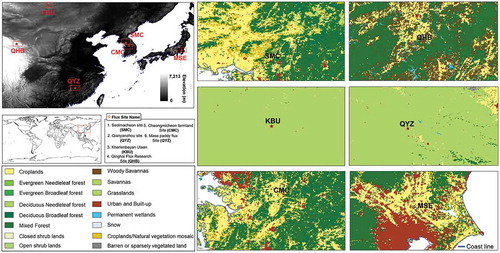
Six sites located in dissimilar topographic and climatic conditions over East Asia were used in this study (Figure 1). The sites are registered in the AsiaFlux network (http://asiaflux.net/) and include two forest sites, i.e. Seolmacheon (SMC, South Korea) and Qianyanzhou (QYZ, South China); two grassland sites, i.e. Kherlenbayan Ulaan (KBU, Mongolia) and Qinghai Flux Research Site (QHB, China); and two cropland sites, i.e. Cheongmicheon farmland site (CMC, South Korea), and a Mase paddy flux site (MSE, Japan). All selected sites differ in meteorological conditions, elevation, vegetation height, measurement height, and climate zones (Table 1). The SMC site, which is located in a temperate zone, has a mean canopy height of 15 m in a mixed forest ecosystem and includes steep mountainous terrain at a mean altitude of 293 m (Kwon et al. 2009). During the summer season (June–August), the Asian monsoon brings intense precipitation associated with high temperature. SMC shows low retention of soil water content (11–20%) because of a thin soil layer, and it demonstrates the importance of root zone soil moisture, which could be a critical factor to sustaining plant growth. In contrast, the QYZ site is located over relatively gentle terrain with a mean altitude of 100 m, wherein the average canopy height reaches as high as 13 m. In contrast to the temperate zone of the SMC site, the QYZ site is located in a subtropical zone as the cumulative mean annual precipitation is relatively higher (1,488.8 mm) and it experiences warmer temperatures and a high-sun season (Yang et al. 2017). The KBU site has a flat terrain with a uniform grassland biome in a semi-arid ecosystem, which is located at a mean elevation of 1,235 m above sea level. The mean annual air temperature (1.2°C) is very low due to low precipitation (<200 mm), 80% of which occurs during the warm season between June and September. On the other hand, the QHB site is located in an alpine meadow ecosystem on the Qinghai–Tibetan plateau, which is also the main water source for central China. The two cropland sites, CMC, and MSE are located in similar climatic conditions with flat terrain. They exhibit an average canopy height <1.2 m. In both sites, the mean annual precipitation reaches 1200 mm, 64% of which is concentrated during the summer monsoon season (June–August). The mean annual air temperatures are 11.5°C and 13.7°C, and the lowest values are −10°C and 1°C for CMC and MSE sites during the winter season, respectively (Liaqat and Choi 2015; Byun, Liaqat, and Choi 2014). Overall, the SMC and QHB sites have complex mountainous regions around them, whereas the other four sites (QYZ, KBU, CMC, and MSE) have flat terrain. The QHB site has the highest elevation (3,250 m) among all six sites used in this study.

Table 1. Specific characteristics of the study area including field and meteorological information (www.asiaflux.net/)

Site	Location		Study period (images)^a	Elevation(Measurement height)^b (m)	Canopy height^c (m)	Vegetation type	Mean annual temperature (°C)	Mean annual precipitation (mm)
	Country	Latitude/Longitude (°N/°E)
Seolmacheon (SMC)	South Korea	37.94/ 126.96	2012 (13)	293 (19.2)	15.0	Mixed forest	10.4	1,332
Qianyanzhou (QYZ)	China	26.73/ 115.07	2003–2004 (11)	100 (23.0)	13.0	Planted forest	18.6	1,488
Kherlenbayan Ulaan (KBU)	Mongolia	47.21/ 108.73	2004–2007 (29)	1,235 (3.5)	0.2	Grassland	1.2	196
Qinghai Flux Research Site (QHB)	China	37.6/ 101.33	2002–2004 (12)	3,250 (2.2)	0.3	Grassland (alpine meadow)	−1.7	567
Cheongmicheon farmland site (CMC)	South Korea	37.16/ 127.65	2012–2013 (9)	141 (10)	1.0	Cropland (rice paddy)	11.5	1,170
Mase paddy flux site (MSE)	Japan	36.05/ 140.03	2002–2004 (23)	13 (3.85)	1.2	Cropland (rice paddy)	13.7	1,200

^aTotal number of Landsat images used in this study along with study years.

^bFlux tower measurement height.

^cAverage vegetation canopy height obtained from in-situ dataset.

Figure 1. The geographical location, ASTER DEM, and land cover map of the study area along with six flux tower sites in East Asia

Flux tower dataset

In-situ flux tower observations obtained from EC systems are used to validate model estimations obtained from two SEBS approaches used in this study. We used half-hourly observations obtained from Asiaflux (http://asiaflux.net) for five sites (i.e. KBU, QHB, CMC, QYZ, and MSE) and from the Hydrological Survey Center of the Republic of Korea for the SMC site (Table 1). The selected sites are equipped with contrasting EC systems such as the open path systems in SMC, KBU, QHB, and CMC sites, whereas combinations of open and closed path EC systems are installed on QYZ and MSE sites with particular measurement heights of 19.2 m (SMC), 23.0 m (QYZ), 3.5 m (KBU), 2.2 m (QHB), 4–10 m (CMC), and 2.5–3.85 m (MSE) sites (Table 1). To observe wind speed, EC systems were equipped with a three-dimensional sonic anemometer (CSAT 3, Campbell) with a combination of infrared gas analyzers (LI-7500, LI-COR) for SMC, QYZ, and QHB sites. Kaijo SAT-550 was used for the KBU site, a three-dimensional sonic anemometer (RM81000) for CMC, and a three-dimensional sonic anemometer (DA600-62AX, KAIJO) was used for the MSE site. Additionally, net radiometers (CNR1, Kipp & Zonen) were installed to observe radiation components. To record the observations, the EC systems used distinct data loggers of a Campbell CR-3000 for SMC, a Campbell CR-5000 for the QYZ site, a Campbell CR-23x for KBU, a digital micrologger (CR-5000, CR23X, Campbell) for QHB, a Campbell CR1000 for CMC, and a DRM3 (TEAC, Tokyo, Japan) for the MSE site. Moreover, EC systems provide surface meteorological parameters such as air temperature, wind speed, atmospheric pressure, relative humidity, and precipitation, which were used to force SEBS and TS-SEBS models in the current study. When coupled with RS-based estimations, instrument-based variables obtained from EC systems provide the dynamics of geophysical processes occurring at the land surfaces. To validate energy terms estimated from both SEBS models, we used the Bowen ratio-corrected, ground-based EC observations (Twine et al. 2000). A flow chart diagram showing the coupling of flux tower-based meteorological datasets and Landsat information along with preprocessing and detailed computational steps are shown in Figure 2.

Figure 2. Flow chart diagram showing key processes involved in preprocessing of ground-based meteorological datasets and Landsat TM/ETM+ images for preparing input into TS-SEBS

Remote sensing dataset

Landsat TM and ETM+

We obtained 97 Landsat TM/ETM+ images from the Global Visualization Viewer United States Geological Survey site (https://glovis.usgs.gov/) for the period of 2002 to 2013. The TM/ETM+ sensors pass through the study sites at local times of 11:00 AM for SMC, 10:30 AM for the QYZ site, 11:30 AM for the KBU site, 11:30 AM for the QHB site, 11:00 AM for CMC, and 10:00 AM for the MSE site. We investigated multiple cloudless images (Table 1), which were coincident with our study period based on data availability. The main reason for selecting only Landsat images for our analysis is that it provides medium-spatial resolution datasets, which provide better ET approximations in heterogeneous regions in comparison with coarser spatial resolution datasets used in literature (Rahman and Zhang 2019; Li et al. 2017; Huang et al. 2015; Byun, Liaqat, and Choi 2014; Wang, Li, and Tang 2013; Lu et al. 2012; Alkhaier, Su, and Flerchinger 2012). To force TS-SEBS, we used RS-based information obtained from Landsat, including normalized difference vegetation index obtained by following the methodology of Allen et al. (2011), surface emissivity (Allen 1996), fractional vegetation coverage (Zhang et al., 2019), canopy height (Chen et al. 2013), leaf area index (LAI), and surface albedo as proposed by Tasumi, Allen, and Trezza (2008). Additionally, land-surface temperature (LST) was calculated using a computationally stable mono-window approach (Qin, Karnieli, and Berliner 2001).

Model formulations and solutions

Description of the TS-SEBS model

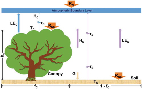
TS-SEBS is a bio-geophysical model derived using the principles of Su (2002) and Monin–Obukhov similarity theory. We integrated LAI-based formulations to partition net radiation (R_N) between soil (R_NS) and canopy (R_NC) and provided estimations of energy budget components of latent heat flux (LE), sensible heat flux (H), and ground heat flux (G). The flowchart of TS-SEBS and comparison with the original SEBS are given in Figure 3, demonstrating the use of Monin–Obukhov similarity theory in its structural algorithm by incorporating reflectances and radiance information obtained from satellite-based estimations with a combination of meteorological datasets to estimate fluxes and land-surface states for both soil and canopy. Depending on the input forcing dataset, TS-SEBS can estimate fluxes over local and regional scales, which highlights the importance of TS-SEBS applications for multi-scale studies. Furthermore, it incorporates an extended model for the determination of roughness lengths using a methodology originally proposed by Su (2001). For original one-source SEBS formulations, the readers are directed to the original article (Su 2002). Here, we only discuss the updated dual-source TS-SEBS model formulations and their solutions. The TS-SEBS scheme is shown in Figure 4, and it is based on the formulations of the energy balance (EB) equation, which is written as follows:

(1) $(R_{NC}+R_{NS})-G=(H_C+H_S)+(L{E}_C+L{E}_S)$(1)

(2) $R_{NC}=R_N(1-ex{p}^{-k_c.LAI})$(2)

(3) $R_{NS}=R_N-R_{NC}$(3)

(4) $R_N=(1-\alpha )R_{S\downarrow }+\epsilon R_{L\downarrow }-\epsilon \sigma LS{T}^4$(4)

Figure 3. Application of original SEBS and updated two-source TS-SEBS proposed in this study

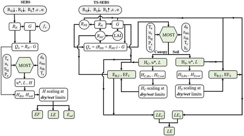
Figure 4. Presents a dual-source scheme in TS-SEBS model

Herein, the subscripts S and C indicate soil and canopy, respectively. LAI (m² m⁻²) is a dimensionless quantity and is equal to foliage area per unit ground area, k_c is a dimensionless extinction coefficient of radiation attenuation within the canopy, α is the surface albedo, $R_{S\downarrow }$ is incoming shortwave radiation, $R_{L\downarrow }$ is downward long wave radiation, $\epsilon$ is surface emissivity, $\sigma$ is the Stefan-Boltzmann constant (5.678x10⁻⁸ Wm⁻²K⁻⁴), and LST is the land-surface temperature derived from Landsat images. A study of the Rio Grande of New Mexico conducted by Trezza, Allen, and Tasumi (2013) showed that the radiation components including estimated using Landsat images under clear sky conditions produce accurate results that are comparable to in-situ measurements.

To estimate G, satellite remote sensing-based methods assume an empirical relationship between G and R_N. For example, the original SEBS parameterizes the ratio of G to R_N using the weighted average of the ratio between bare soil and full vegetation canopies based on fractional vegetation coverage by following the methodology suggested by Kustas and Daughtry (1990). Previous methods used to model G incorporated the fractional vegetation cover-based formulation. This method was reported to provide inaccurate estimations in dense vegetation canopies due to its tendency to saturate much faster in those areas (Timmermans et al. 2013). To circumvent this limitation, Kustas, Daughtry, and V (1993) proposed a new LAI-based formulation that is reliable since it considers the extinction of incoming solar radiation. Therefore, we used an improved LAI-based formulation to estimate G as follows:

(5) $G=0.34\times R_N\times exp(-0.46\times LAI)$(5)

TS-SEBS was employed to estimate H using the Monin–Obukhov similarity theory under dry and wet limits for bare soil as well as canopy components by following the approach of Su (2002). It is noteworthy that aerodynamic resistances were computed from formulations of Sánchez et al. (2008), which were adapted from formulations used by Norman, Kustas, and Humes (1995), Kustas and Norman (1999a), Brutsaert (1999), and Li et al. (2005). The canopy temperature (T_c) was derived from Yang et al. (2018b). The mathematical formulations are as follows:

(6) $H_C=k{u}_{\ast }\rho c_p\left({\theta }_c-{\theta }_a\right)/\left[{r_a}^h\right]$(6)

(7) $H_S=k{u}_{\ast }\rho c_p\left({\theta }_s-{\theta }_a\right)/\left[{r_a}^a+{r_a}^s\right]$(7)

(8) $r_C=\frac{\left[ln\left(\frac{z_u-d_0}{z_{0m}}\right)-{\mathrm{\Psi }}_m\left(\frac{z_u-d_0}{L}\right)+{\mathrm{\Psi }}_m\left(\frac{z_{0m}}{L}\right)\right]\times \left[ln\left(\frac{z_T-d_0}{z_{0h}}\right)-{\mathrm{\Psi }}_h\left(\frac{z_T-d_0}{L}\right)+{\mathrm{\Psi }}_h\left(\frac{z_{0h}}{L}\right)\right]}{k^{2}u}$(8)

(9) $r_a=\frac{\left[ln\left(\frac{z_u-d_0}{z_{0m}}\right)-{\mathrm{\Psi }}_m\right]\left[ln\left(\frac{z_u-d_0}{z_{0m}}\right)-{\mathrm{\Psi }}_h\right]}{k^{2}u}$(9)

(10) $r_S=\frac{1}{0.00025{(T_s-T_c)}^{1/3}+0.012u_s}$(10)

(11) $T_c=T_a+\frac{\left[R_{NC}{r}_a\right]}{\rho c_p}\left[1-\alpha f_c\frac{\mathrm{\Delta }}{\mathrm{\Delta }+\gamma }\right]$(11)

(12) $f_C=\frac{NDVI-NDV{I}_{min}}{NDV{I}_{max}-NDV{I}_{min}}$(12)

(13) $L=\frac{\rho c_p{u_{\ast }}^3{\theta }_v}{kgH}$(13)

Here, k is the von Karman constant with a value of 0.41;$u_{\ast }$ is the friction velocity (ms⁻¹); ρ is the density of air (kgm⁻³); c_p is the air specific heat capacity (J kg⁻¹ K⁻¹);${\theta }_s$,${\theta }_c$,, and ${\theta }_a$ are potential surface, canopy, and air temperatures, respectively, and were estimated using the method of Brutsaert (2005). In the above equations, z_u and z_T are measurement heights (m) for wind speed (u) and air temperature (T_a), respectively; d₀ is zero-plane displacement height, and ${\mathrm{\Psi }}_h$ and ${\mathrm{\Psi }}_m$ are stability correction functions for heat and momentum transfer whose derivation is mentioned in Sánchez et al. (2008). Air temperature and atmospheric pressure obtained from in-situ flux tower sites were used to estimate ${\theta }_a$. ${\theta }_c$ was estimated using T_c. ${\theta }_s$ was computed from the LST obtained from Landsat images (section 2.3.1). ${\theta }_v$ is the atmospheric virtual potential temperature in Kelvin. f_c is the canopy fraction estimated as described by Chen et al. (2013). α is the Priestley Taylor coefficient, Δ is the slope of the saturation vapor pressure versus temperature curve (kPa/°C), and $\gamma$ is the psychrometric constant (kPa/°C). u_s is wind speed above the soil surface, where soil roughness does not affect free wind movement, which was estimated using logarithmic wind profiles from Kustas and Norman (1999b). r_c is the aerodynamic resistance to heat transfer between the canopy and reference height, r_a is the aerodynamic resistance of air, and r_s is the aerodynamic resistance above soil surfaces. Details related to these resistance terms are mentioned in Sánchez et al. (2008). Finally, L is the Obukhov length. The TS-SEBS model uses an iterative process in order to find all unknown parameters such as L, $u_{\ast }$, and H separately for both soil and canopy fractions.

The roughness length for momentum transfer (z_0m) and kB⁻¹ was obtained from improved formulations of Chen et al. (2013). Specifically, the three elements of kB⁻¹ including canopy, water, and mixed canopy and soil components were obtained from Chen et al. (2014). Accurate canopy height measurements obtained from ground-based observations were used in this study to estimate canopy height (h_c). Finally, an extended model obtained from Su (2002) was used for estimation of the roughness length for heat transfer (z_0h). The detailed formulations of z_0h, z_0m, and kB⁻¹ are as follows:

(14) $z_{0h}=\frac{z_{0m}}{exp(k{B}^{-1})}$(14)

(15) $z_{0m}=h_c\left(1-\frac{d_0}{h_c}\right)exp\left(-\frac{k}{\beta }\right)$(15)

(16) $k{B}^{-1}={f_c}^2\times k{B_c}^{-1}+{f_s}^2\times k{B_s}^{-1}+2\times f_c\times f_s\times k{B_m}^{-1}$(16)

Here, β represents the ratio of frictional velocity to wind speed; f_s is the complement of f_c (f_s = 1-f_c); kB⁻¹ is a dimensionless heat transfer coefficient called the inverse Stanton number, and the subscripts c, s, and m represent the canopy, soil, and mixed canopy and soil in the study region, respectively. It is important to mention that TS-SEBS used an updated wind speed profile extinction coefficient from Massman, Forthofer, and Finney (2017), which was used to estimate z_0h and d₀, which is in contrast with the Massman (1996) formulation used in the original one-source SEBS.

After computation of G and H components, LE was estimated from Eq. (1)(1) $(R_{NC}+R_{NS})-G=(H_C+H_S)+(L{E}_C+L{E}_S)$(1) for soil as follows:

(17) $L{E}_S=E{F}_S(R_{NS}-G)$(17)

(18) $E{F}_S=eva{p}_{r,S}\frac{(R_{NS}-G-H_{wet,S})}{R_{NS}-G}$(18)

(19) $eva{p}_{r,S}=1-\frac{(H_S-H_{wet,S})}{H_{dry,S}-H_{wet,S}}$(19)

(20) $H_{wet,S}=\left((R_{NS}-G)-\frac{\rho C_p}{R_{SW}}.\frac{P_{Sat}-P_{Vap}}{\gamma }\right)/\left(1+\frac{\mathrm{\Delta }}{\gamma }\right)$(20)

(21) $H_{wet,\mathrm{S}}=R_{NS}-G$(21)

(22) $R_{SW}=\frac{1}{k{u}_{\ast }}\left[ln\left(\frac{z-d_0}{z_{0h}}\right)-{\mathrm{\Psi }}_h\left(\frac{z-d_0}{L_{Wet,S}}\right)+{\mathrm{\Psi }}_h\left(\frac{z_{0h}}{L_{Wet,S}}\right)\right]$(22)

(23) $L_{Wet,S}=-\frac{\rho {u_{\ast }}^3}{kg0.61(R_{N,S}-G)/\lambda }$(23)

where H_wet,S and H_dry,S are the H estimations at wet and dry limits, R_SW is the external resistance to heat transport over the soil at the wet limit, L_wet,S is the Obukhov length at the wet limit, and λ is the latent heat of vaporization with a value of 2.26 MJ kg⁻¹. Similarly, LE was estimated for canopy components as follows:

(24) $L{E}_C=E{F}_C(R_{NC})$(24)

(25) $E{F}_C=eva{p}_{r,C}\frac{(R_{NC}-H_{wet,C})}{R_{NC}}$(25)

(26) $eva{p}_{r,C}=1-\frac{(H_C-H_{wet,C})}{H_{dry,C}-H_{wet,C}}$(26)

(27) $H_{wet,C}=\left((R_{NC})-\frac{\rho C_p}{R_{CW}}.\frac{P_{Sat}-P_{Vap}}{\gamma }\right)/\left(1+\frac{\mathrm{\Delta }}{\gamma }\right)$(27)

(28) $H_{dry,C}=R_{NC}$(28)

(29) $R_{CW}=\frac{1}{k{u}_{\ast }}\left[ln\left(\frac{z-d_0}{z_{0h}}\right)-{\mathrm{\Psi }}_h\left(\frac{z-d_0}{L_{Wet,C}}\right)+{\mathrm{\Psi }}_h\left(\frac{z_{0h}}{L_{Wet,C}}\right)\right]$(29)

(30) $L_{wet,C}=-\frac{\rho {u_{\ast }}^3}{kg0.61(R_{N,C})/\lambda }$(30)

where L_wet,C is the Obukbov length of wet canopies. TS-SEBS assumes that LE is zero in the theoretical wet limit of sensible heat flux over the soil, H_wet,S, which means that all incoming net radiation is partitioned between sensible heat flux and ground heat flux over the soil surface. The EF computed in TS-SEBS was appropriate for nonadvection conditions (such as natural vegetation) in contrast with irrigated regions where water inputs change with time.

Scaling up method of instantaneous ET

After estimating instantaneous LE from both soil and canopy components, instantaneous ET can be obtained at the Landsat revisit time. Few studies have used diurnal variations in EF to estimate the daily ET (Farah, Bastiaanssen, and Feddes 2004). However, in the estimation of daily ET, TS-SEBS assumes that the EF computed for each soil and canopy fraction was constant throughout the day (Liaqat and Choi 2017; Byun, Liaqat, and Choi 2014; Jia et al. 2009; Su 2002; Crago and Brutsaert 1996). Therefore, the daily ET was scaled from instantaneous LE and EF for both soil and canopy components as follows:

(31) $E{F}_S=\frac{L{E}_S}{R_{NS}-G}$(31)

(32) $E{T}_{Daily,S}=8.64\times {10}^7\times E{F}_S\times \frac{R_{N24}-G_{24}}{\lambda {\rho }_w}$(32)

(33) $E{F}_C=\frac{L{E}_C}{R_{NC}}$(33)

(34) $E{T}_{Daily,C}=8.64\times {10}^7\times E{F}_C\times \frac{R_{N24}}{\lambda {\rho }_w}$(34)

Here, $R_{N24}$ is daily net radiation, $G_{24}$ is daily ground heat flux, and ${\rho }_w$ is water density (kg m⁻³). Equations (1)(1) $(R_{NC}+R_{NS})-G=(H_C+H_S)+(L{E}_C+L{E}_S)$(1) to (30) constitute TS-SEBS model formulations, whereas Eqs. (31)(31) $E{F}_S=\frac{L{E}_S}{R_{NS}-G}$(31) to (34) represents daily ET estimations from each soil and canopy component.

Flux tower footprint modeling

The flux tower footprint represents the area that contributes to flux observations. Estimation of the footprint requires several input datasets such as atmospheric stability, wind speed, wind direction, and measurement heights. Previous studies reported that spatial discrepancies may arise during validation of estimations obtained from high-resolution remote sensing retrievals compared with local scale flux tower observations (Ma et al. 2018), which suggests footprint modeling must be conducted prior to data validations to avoid those spatial discrepancies. Jia et al. (2012) and Bai et al. (2015) suggested using pixels of high-resolution remote sensing estimations that are under the source area of flux towers for validation. This means that validation pixels could include several pixels. Considering the literature, we selected an analytical two-dimensional flux tower footprint model for estimating the source area of six selected flux tower sites by following the methodology of Hsieh, Katul, and Chi (2000). After footprint modeling, we aggregated the TS-SEBS model outputs and selected only those validation pixels under the source area of the flux tower sites to establish a fair comparison (Song et al. 2020).

Model performance evaluation

To validate TS-SEBS estimations and compare them with independent flux tower observations, we selected four statistical indicators of bias, root-mean-square error (RMSE), Pearson’s correlation coefficient (R), and normalized standard deviation (σ_n), which are described as follows:

(35) $\mathrm{B}\mathrm{i}\mathrm{a}\mathrm{s}=\frac{1}{N}\sum _{i=1}^N(S_i-O_i)$(35)

(36) $\mathrm{R}\mathrm{M}\mathrm{S}\mathrm{E}=\hspace{0.17em}\sqrt{\frac{\sum _{i=1}^N{(S_i-O_i)}^2}{N}}$(36)

(37) $\mathrm{R}=\frac{\sum _{i=1}^N{(S_i-\bar{S})}^2{(O_i-\bar{O})}^2}{\sqrt{\sum _{i=1}^N{(S_i-\bar{S})}^2}\sqrt{\sum _{i=1}^N{(O_i-\bar{O})}^2}},-1\le \mathrm{R}\le +1$(37)

(38) ${\sigma }_n={\sigma }_{model}/{\sigma }_{in-situ}$(38)

Here, S is the simulated value, O is the observed value, $\bar{O}$ represents the mean observed value, and $R_{N24}$ is the mean-simulated value. The subscript i denotes sample number, and N denotes a total number of samples. The ${\sigma }_n$ denotes standard deviation with subscript n representing “normalized.” RMSE indicates the variations of residuals around the best fit line, which demonstrates the variations in predicted and observed means (Legates and McCabe 1999). Moreover, we used time series analysis, scatter plot analysis, and a Taylor diagram (Taylor 2001) for detailed investigation of model accuracies. The Taylor diagram uses R and ${\sigma }_n$ collectively in a two-dimensional space to produce an effective tool to summarize and compare multiple model performances in comparison with ground-based flux tower observations.

Results and discussion

Quantitative and qualitative evaluation of models

Evaluation of radiation components

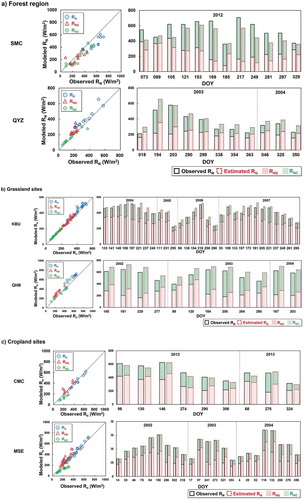
To evaluate the accuracy of the TS-SEBS model in estimating and partitioning of R_N into the soil (R_NS) and canopy (R_NC) components, we used EC based in-situ datasets and compared these with model estimations at corresponding footprint locations of flux tower sites. The statistical results in the form of scatter plots and bar charts are presented in Figure 5. As shown, the distributions of three radiation components and their comparison with flux tower observations are portrayed for three geophysical land cover types. The results reveal that the estimated radiation components very well capture the seasonal trends since all radiation components showed high values during higher sun seasons (i.e. summer) when LAI values are at their peaks starting from April to September. Relatively lower values were observed in cloudy and snowfall periods when LAI values were lower, during the winter seasons starting from October to March. This better agreement in the seasonal trend is the reason that all scatter points are clustered along with the identity (1:1) line. The statistical comparison metrics as presented in Table 2, showing mean bias and RMSE of 10.90 Wm⁻² and 58.95 Wm⁻² for R_N, 35.14 Wm⁻², and 63.35 Wm⁻² for R_NS, and −25.06 Wm⁻², and 45.93 Wm⁻² for R_NC components, respectively, for six selected sites. For the forest (SMC) site, an RMSE of 107.71 Wm⁻² was observed. In a previous study, Byun, Liaqat, and Choi (2014) obtained an RMSE of 128.46 Wm⁻² in the same SMC site using coarse-resolution surface reflectance information from MODIS (Moderate Resolution Imaging Spectroradiometer) with a spatial resolution of 1 km and meteorological inputs from GLDAS datasets with a spatial resolution of 25 km. Therefore, our improved results demonstrate that the incorporation of fine-resolution input datasets (30 m) into TS-SEBS yielded better flux estimations. This was corroborated by a study reported by Badgley et al. (2015), which demonstrated that incorporation of fine- versus coarse-resolution input datasets into an ET model can significantly improve the estimated heat fluxes. The SMC and QYZ sites showed underestimation and overestimation of R_N due to underestimation and overestimation of R_NS and R_NC components, respectively (Table 2). In grassland sites, overestimations of all radiation components (i.e. R_N, R_NS, and R_NC) were observed with mean bias and RMSE values ranging from 4.85 to 54.86 Wm⁻² and from 16.49 to 61.14 Wm⁻², respectively. The mean-estimated radiation components were closer to mean in-situ observations in cropland sites, followed by forest and grassland sites. This is because of the homogeneity in the cropland ecosystem compared with forest and grassland sites, which facilitates estimation of heat fluxes by EC sensors. On the other hand, the relatively larger difference between mean estimated radiation components and in-situ observations in two distinct grassland sites was attributed to geographical location and complexity in estimating fluxes in those regions. This is due to the arid ecosystem location of one site (KBU), which showed relatively better estimations, with a difference in mean R_N values of 24.29 Wm⁻². Another site (QHB) is located in the complex mountainous region at the highest altitude of the Qinghai-Tibetan plateau, with a relatively larger difference in a mean R_N value of 86.91 Wm⁻². Our results reveal that the complexity involved in flux tower sites directly influences the estimation of radiation components. Our results further reveal that the model produced better estimations of radiation components in arid ecosystems in comparison with the complex high-altitude mountainous landscape of the Qinghai-Tibetan plateau. Similarly, the two cropland sites showed an underestimation pattern of R_N with a mean bias value of −8.19 Wm⁻², which was attributed to the underestimation of R_NC (Table 2). The underestimation of R_NC in cropland sites is explained as follows. TS-SEBS uses an LAI-based formulation to partition R_N into soil and canopy components; however, the estimated LAI values are lower, with a mean of 0.93 m²/m². Additionally, the obtained RMSE was lower, with a mean value of ~73 Wm⁻² (Table 2), which may be responsible for its underestimation. Overall, R_N showed a relatively larger RMSE in the complex forest sites due to higher spatial heterogeneity. Grassland and cropland sites showed the next highest RMSE values, which are related to the difficulties of remote sensors during estimation of R_N surface reflectance values such as LST, emissivity, and albedo fractions (Chen et al. 2019; Ma et al. 2018; Byun, Liaqat, and Choi 2014; Lu et al. 2012).

Table 2. Statistical comparison of observed radiation components with modeled instantaneous net radiation (R_N) along with its partitioning at soil (R_NS) and canopy (R_NC) and ground heat flux at six flux tower sites. All units are in W/m^2.

Land cover type	Site		Mean (in-situ)	Mean (model)	Bias	RMSE
Net radiation (RN)
Forest	SMC	RN	550.85	464.74	−86.11	107.71
		RNS	257.93	220.29	−37.65	78.38
		RNC	292.91	244.46	−48.47	71.09
	QYZ	RN	343.3	401.49	58.18	68.82
		RNS	194.67	246.75	52.09	63.04
		RNC	148.63	154.72	6.08	34.38
Grassland		RN	399.65	423.94	24.20	32.99
	KBU	RNS	283.76	301.49	17.68	24.09
		RNC	115.89	122.47	6.54	9.17
		RN	553.93	640.83	85.51	89.32
	QHB	RNS	237.49	317.95	82.23	83.93
		RNC	316.44	322.87	3.15	23.82
Cropland		RN	459.64	439.18	−21.2	29.87
	CMC	RNS	269.86	310.05	37.15	57.58
		RNC	189.79	129.18	−58.35	64.09
		RN	436.36	441.42	4.82	25.02
	MSE	RNS	246.28	307.19	59.35	73.02
		RNC	190.08	129.17	−59.36	73.08
Ground heat flux (G)
Forest	SMC		102.92	96.75	1.74	42.86
	QYZ		75.17	93.75	18.55	22.08
Grassland	KBU		53.88	111.59	57.74	75.74
	QHB		81.31	128.36	47.05	50.85
Cropland	CMC		12.53	119.01	106.46	109.26
	MSE		69.23	11.32	42.07	54.51

Figure 5. Comparison of in-situ radiation components with modeled instantaneous net radiation (R_N), modeled R_N over soil (R_NS), and modeled R_N over canopy (R_NC) at two forest (SMC and QYZ) sites. Comparison of in-situ radiation components with modeled instantaneous net radiation (R_N), modeled R_N over soil (R_NS), and modeled R_N over canopy (R_NC) at two grassland (KBU and QHB) sites. Comparison of in-situ radiation components with modeled instantaneous net radiation (R_N), modeled R_N over soil (R_NS), and modeled R_N over canopy (R_NC) at two cropland(CMC and MSE) sites

Evaluation of ground heat flux between in-situ and SEBS models

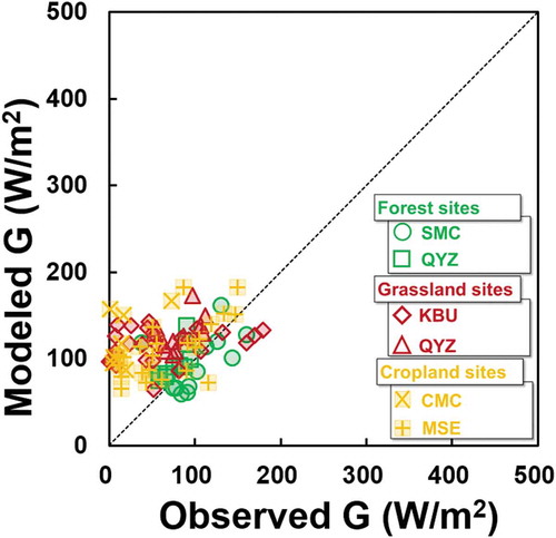
Ground heat flux (G) is an important parameter in closing the energy budget since it is used for partitioning of available energy (R_N-G) into H and LE components. To validate the estimated G obtained from TS-SEBS, we used ground-based G observations from flux towers. However, we could not find reliable flux tower datasets for forest sites (i.e. SMC and QYZ) due to malfunctioning of plates measuring G. To validate estimated G for forest sites, we used R_N from in-situ observations, estimated the leaf area index using the methodology of (Su 2002) by incorporating medium-resolution Landsat TM/ETM images. Finally, we used improved formulations by Kustas, Daughtry, and Oevelen (1993) and Timmermans et al. (2013) to estimate ground-based G. The results of scatter plot analysis are presented in Figure 6, which shows a reliable-estimated G, with all estimations close to the identity line. However, the two SEBS approaches consistently overestimated G in all six selected sites in this study, with mean bias and RMSE values of 45.60 Wm⁻² and 59.21 Wm⁻², respectively (Table 2). This corroborates the findings reported in Liaqat and Choi (2015). This corroboration and better-estimated G obtained in the current study revealed that our approach can be used as an alternative method to estimate ground-based G when in-situ observations are unavailable due to malfunctions or bad environmental conditions such as storms or intense rainfall events. Our models in comparison with EC observation demonstrated a relatively larger error in CMC cropland sites, which is explained by the larger positive bias (106.46 Wm⁻²) in the measurements. This larger error was attributed to the relatively lower surface temperature of the earth due to environmental conditions based on the selection of five of 9 days at the CMC site (Figure 5c) from the winter season starting from November to March in South Korea. These days were characterized by low surface temperature due to lower air temperature and snowfall seasons. In such atmospheric conditions, the remote sensing-based G estimations tended to overestimate ground-based observations since the flux tower plates used to measure G tends to produce lower observation values (Figure 6). This is in agreement with a previous study comparing six models for G estimations at 88 global flux tower sites, finding greater intermodal uncertainty in the winter season (Purdy et al. 2016). It is important to mention that we did not use a fractional vegetation cover-based formulation of G because it saturates much faster in dense vegetation conditions. Therefore, we used an LAI-based formulation for G to provide better estimations (Timmermans et al. 2013). Overall, the better performance of G in all six selected sites is due to the incorporation of improved LAI-based formulations in the structural algorithm of the updated TS-SEBS model, which provides reliable estimates (Kustas, Daughtry, and Oevelen 1993), since it effectively considers extinction of solar incoming radiation in the canopies.

Figure 6. Comparison of in-situ and estimated ground heat flux (G) at two forest (SMC and QYZ), two grassland (KBU and QYZ), and two cropland sites (CMC and MSE)

Evaluation of components of sensible heat flux

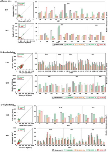
Estimation of sensible heat flux (H) at regional scales from remote sensing information has always been challenging (Liaqat and Choi 2015) because it is related to the exchange of heat in terms of conduction and convection processes, making it difficult to determine in heterogeneous areas. A comparison of estimated H from TS-SEBS and SEBS approaches is shown using scatter plot analysis and bar charts in Figure 7 for three ecosystem sites. A comparison of the bar charts in Figure 7 shows that overall sensible heat fluxes from the canopy (H_C) contribute more to total H estimations in those sites. Day of the year (DOY) in the growing season is correlated with an increase in LAI. This is explicitly due to the reduction of aerodynamic resistances with an increase in LAI and the number of leaves, which in turn increases H_C (Deguchi, Hattori, and Park 2006). The statistical results as presented in Table 3 show that the respective mean bias and RMSE values are 2.32 Wm⁻² and 57.83 Wm⁻² for TS-SEBS and −20.68 Wm⁻² and 79.47 Wm⁻² for SEBS estimations, a ~ 27% difference. This relatively better performance of TS-SEBS in characterizing H components reveals that its updated parameters using LAI for estimation of H components (over soil and canopy) accurately reflect seasonal changes in canopies compared with the original SEBS model. This is why TS-SEBS (in comparison with SEBS) demonstrated better estimates of turbulent heat fluxes over heterogeneous East Asian ecosystems. TS-SEBS showed overestimation patterns, while SEBS produced underestimation, in agreement with previous studies (Chen et al. 2019; Liaqat and Choi 2015; Gokmen et al. 2012). The reason for this underestimation pattern of H in SEBS is the underlying algorithm, which is based on Monin–Obukhov similarity theory (Arnqvist and Bergström 2015) and attributed to underestimation of momentum fluxes. The relatively lower mean bias and RMSE values of TS-SEBS compared with SEBS can be explained as follows. The model performances of SEBS and TS-SEBS are dependent on kB^−1, more specifically EF, which may cause uncertainties in estimated H. We incorporated an improved kB⁻¹ formulation proposed by Chen et al. (2014) to produce better flux estimations. Moreover, the relatively better agreement of H by TS-SEBS is due to the incorporation of an improved canopy wind model in its structural algorithm (Massman, Forthofer, and Finney 2017), in contrast with the Massman (1996) approach used in SEBS. Canopy height also plays a critical role in estimating aerodynamic resistances, which is key for H estimation using remote sensing information. TS-SEBS separately calculated aerodynamic resistances for canopy, soil, and air (section 3.1), in contrast with the lumped resistance produced by SEBS, resulting in relatively better H estimations.

Table 3. Statistical comparison of mean in-situ and estimated sensible heat flux (H), Latent heat flux (LE), and daily ET along with their partitioning at soil and canopy components at six flux tower sites in Asia

		In-situ	TS-SEBS model					SEBS model
Land cover type	Site	Mean H(in-situ)	Mean H (model)	Mean Hs (model)	Mean Hc(model)	Bias(W/m^2)	RMSE(W/m^2)	Mean H(model)	Bias(W/m^2)	RMSE(W/m^2)
Sensible heat flux (H), Unit in W/m^2
Forest	SMC	91.92	108.61	61.98	46.62	11.33	80.18	93.34	1.41	105.26
	QYZ	123.21	141.35	110.96	30.39	16.63	76.01	107.67	−14.24	105.16
Grassland	KBU	144.86	195.77	139.49	56.27	−67.10	34.41	189.12	−73.76	97.57
	QHB	133.95	135.84	34.29	101.55	1.89	43.53	111.04	1.89	43.53
Cropland	CMC	123.01	153.24	73.50	79.74	30.22	57.16	98.59	−24.42	64.86
	MSE	74.97	144.69	85.23	59.46	20.95	55.72	108.76	−14.97	60.47
Land cover type	Site	Mean LE(in-situ)	Mean LE (model)	Mean LEs (model)	Mean LEc(model)	Bias(W/m^2)	RMSE(W/m^2)	Mean LE(model)	Bias(W/m^2)	RMSE(W/m^2)
Instantaneous Latent heat flux (LE), Unit in W/m^2
Forest	SMC	246.66	292.40	101.16	191.24	45.74	134.80	274.62	27.96	152.86
	QYZ	161.16	200.16	57.24	142.92	39.01	75.66	210.80	49.64	81.07
Grassland	KBU	85.08	127.33	60.44	66.89	35.64	66.03	135.74	43.47	76.22
	QHB	274.09	380.26	160.84	219.42	106.17	122.73	405.07	130.98	138.16
Cropland	CMC	219.30	183.54	131.25	52.29	−35.75	76.98	237.25	17.92	84.05
	MSE	133.86	177.14	108.74	68.39	43.27	90.09	211.67	77.81	129.73
Land covet type	Site	Mean ET(in-situ)	Mean ET (model)	Mean Es (model)	Mean Tc(model)	Bias(mm/day)	RMSE(mm/day)	Mean ET(model)	Bias(mm/day)	RMSE(mm/day)
Daily ET and its component at soil (Es) and canopy (Tc), Unit in mm/day
Forest	SMC	2.30	2.34	0.96	1.38	−0.14	1.56	2.31	−0.17	1.66
	QYZ	2.27	2.05	0.84	1.22	−0.22	0.87	2.13	−0.14	0.97
Grassland	KBU	1.07	1.93	1.13	0.80	0.81	1.14	2.16	1.03	1.46
	QHB	3.52	4.63	2.52	2.11	1.11	1.87	4.82	1.32	1.87
Cropland	CMC	2.88	2.41	1.94	0.48	0.64	0.87	2.96	1.19	1.40
	MSE	3.03	1.96	1.39	0.56	−0.36	0.86	2.33	0.02	0.88

Figure 7. Comparison of in-situ sensible heat flux (H) with modeled estimations from TS-SEBS and SEBS approaches. The partitioning of H using TS-SEBS in to soil (H_S) and canopy (H_C) component is shown using box plot at two forest (SMC and QYZ) sites, two grassland (KBU and QHB) sites, and two cropland (CMC and MSE) sites

It is noteworthy that, the MOST theory, on which the TS-SEBS model is based, was typically developed for uniform or flat surfaces, which may induce uncertainties in complex topography (Arnqvist and Bergström 2015) if the fluxes were modeled by using coarse spatial resolution input datasets. In order to circumvent the limitation of the MOST theory in complex topography and make it suitable to use for multiple land cover types, the TS-SEBS used in its structural algorithm the updated wind speed profile extinction coefficient formulation from Massman, Forthofer, and Finney (2017) and integrated medium-scale 30 m spatial resolution satellite information from Landsat to model improved fluxes. Additionally, comparing to semi-empirical-based formulation of aerodynamic conductance used by SEBS which causes uncertainties in estimated heat fluxes (Bhattarai et al. 2016), the improved TS-SEBS model uses a more physical-based formulation of aerodynamic conductance by Sánchez et al. (2008). This improved aerodynamic conductance formulation in TS-SEBS as well as separately calculating heat fluxes for both soil and canopy components may be the reason for improved accuracy in various land cover types investigated in the current study.

Evaluation of components of latent heat flux

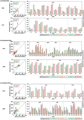
Based on the residual energy budget formulation (Eq. 1(1) $(R_{NC}+R_{NS})-G=(H_C+H_S)+(L{E}_C+L{E}_S)$(1) ), the two models used in this study (TS-SEBS and SEBS) estimated instantaneous latent heat flux (LE) and were compared with in-situ flux tower observations. The results in terms of scatter plots and bar charts are presented in Figure 8 for the forest, grassland, and cropland sites. These illustrate good estimates for LE since seasonal variations are well captured to demonstrate high values during the growing season and low values during the winter season, in which all values are closer to the identity line. As shown in Figure 8, a comparison of the bar charts demonstrates detailed partitioning of LE into the soil (LE_S) and canopy (LE_C) components, which further reveals that LE_C has a stronger influence on total LE estimation since its values are greater than those of LE_S. The relatively larger values of LE_C compared with LE_S are because all sites are located in vegetated ecosystems, where NDVI is higher compared with that of bare soil. The vegetated regions have high NDVI due to higher chlorophyll content because of maximum plant transpiration. This results in an increase in LE_C, yielding a relatively higher LE_C compared with LE_S. On the other hand, SEBS is unable to partition LE between soil and canopy since its baseline algorithm was developed by their integration as a single component. This is in contrast to TS-SEBS, which divides the two regimes, and separately calculates the components of LE for soil and canopy. This is one advantage of TS-SEBS, namely, that we can conduct an in-depth analysis of LE as well as its partitioning into soil and canopy fractions. This may play a key role in accurately estimating the components of turbulent heat fluxes. The statistical analysis metrics presented in Table 3 reveal that both TS-SEBS and SEBS models showed overall good agreement compared with in-situ observations. Overall, the respective mean bias and RMSE values are 39.01 Wm⁻² and 94.38 Wm⁻² for TS-SEBS and 57.96 Wm⁻² and 110.34 Wm⁻² for the SEBS model. These statistics further reveal the significantly improved performance of TS-SEBS compared with SEBS due to a reduction in RMSE since its mean RMSE is lower than that of SEBS by 15.96 Wm⁻² (~14%). It is worth mentioning that the original SEBS model overestimated LE in all six sites, with mean bias and RMSE values ranging from 17.92 to 130.98 Wm⁻² and from 76.22 to 152.86 Wm⁻², respectively. In contrast, the TS-SEBS model showed overestimation patterns in all selected sites except CMC, in which it showed an underestimation pattern with a mean bias value of −35.75 Wm⁻². Underestimation of LE in the CMC site corroborates a study conducted by Byun, Liaqat, and Choi (2014), with a bias value of −119.17 Wm⁻² using coarse-resolution MODIS and GLDAS datasets. This can be compared with the improved bias value of −35.75 Wm⁻² in the current study, obtained using medium-spatial resolution Landsat images, which highlighted the importance of introducing fine spatial resolution satellite information to retrieve accurate turbulent heat fluxes. Overall, overestimation of LE by SEBS was reported in previous studies (Chen et al. 2019; Ma et al. 2018; Gokmen et al. 2012) due to underestimation of turbulent sensible heat fluxes (Table 3). The statistics of individual sites reveal overall higher RMSE values for SMC, which may be attributed to its relatively higher canopy height (15 m) compared with the five other sites. This is because the higher canopy height in the heterogeneous landscape results in higher resistance to LE, which in turn produces higher RMSE in the estimated heat fluxes. Overall, both TS-SEBS and SEBS models showed acceptable accuracies compared with independent ground-based flux tower observations, and these results are in agreement with previous studies (Zhao et al. 2019; Ma et al. 2018; Webster, Ramp, and Kingsford 2017; Liaqat and Choi 2017; Byun, Liaqat, and Choi 2014; Chen et al. 2013; Gokmen et al. 2012).

Figure 8. Comparison of in-situ Latent heat flux (LE) with modeled estimations from TS-SEBS and SEBS approaches. The partitioning of LE using TS-SEBS in to soil (LE_S) and canopy (LE_C) component is shown using box plot at two forest sites (SMC, QYZ). Comparison of in-situ Latent heat flux (LE) with modeled estimations from TS-SEBS and SEBS approaches. The partitioning of LE using TS-SEBS in to soil (LE_S) and canopy (LE_C) component is shown using box plot at two grassland sites (KBU and QHB). Comparison of in-situ Latent heat flux (LE) with modeled estimations from TS-SEBS and SEBS approaches. The partitioning of LE using TS-SEBS in to soil (LE_S) and canopy (LE_C) component is shown using box plot at two cropland sites (CMC and MSE)

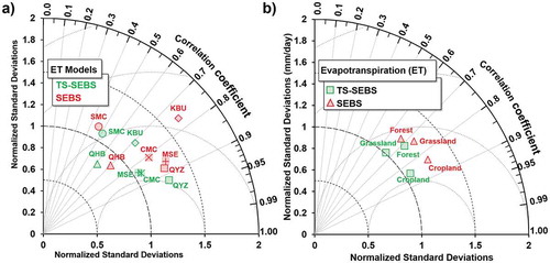
TS-SEBS considers instantaneous LE in conjunction with EF to estimate daily ET for both soil (E_S) and canopy (T_C) components. The results of scatter plot analysis and bar charts are presented in Figure 9a, 9b, and 9c for the forest, grassland, and cropland sites, respectively. These figures show that both TS-SEBS and SEBS models demonstrate good agreement with flux tower observations, with values falling close to the identity line. The bar chart shows the partitioning of ET into its soil (E_S) and canopy (T_C) components for both selected sites, further demonstrating that the estimated ET very well captured the seasonal trends, with a large ET in the growing season and low ET during the winter season. Bar charts reveal that, in comparison with E_S, T contributes more to total ET estimation in the two selected forest sites compared with cropland and grassland sites. This is natural since selected forest sites have greater canopy fractions compared with soil components due to the forest ecosystem. These results further reveal higher ET values in growing and high-sun periods of the year (Figure 9). A comprehensive summary of the validation statistics is presented in Table 3, which shows that mean bias and RMSE values of 0.30 mm/day and 1.19 mm/day for TS-SEBS, respectively, and of 0.54 mm/day and 1.37 mm/day for the SEBS model. These statistics further reveal the improved performance of TS-SEBS compared with SEBS in simulating ET, since it showed a reduction in RMSE by ~13%. The mean ET obtained from both selected models showed good agreement compared with observed averages from flux tower sites (Table 3). Thus, both models accurately represent simulated ET at selected sites in this study. The results obtained from the Taylor diagram analysis as presented in Figure 10 demonstrate that the TS-SEBS tends to perform better than SEBS due to its improvement in R and σ_n values. For example, the mean R and σ_n values were 0.75 and 1.08, respectively, for TS-SEBS and 0.73 and 1.25 for the SEBS model. These statistics reveal that, in comparison with SEBS, TS-SEBS showed a ~ 3% increase in R and a ~ 14% decrease in mean σ_n toward unity, which more closely approximates the actual EC observations obtained from in-situ flux towers.

Figure 9. Comparison of in-situ Evapotranspiration (ET) with modeled estimations from TS-SEBS and SEBS approaches. The partitioning of ET using TS-SEBS in to soil (E_S) and canopy (T_C) component is shown using box plot at two forest (SMC, QYZ) sites. Comparison of in-situ Evapotranspiration (ET) with modeled estimations from TS-SEBS and SEBS approaches. The partitioning of ET using TS-SEBS in to soil (E_S) and canopy (T_C) component is shown using box plot at two grassland (KBU, QHB) sites. Comparison of in-situ Evapotranspiration (ET) with modeled estimations from TS-SEBS and SEBS approaches. The partitioning of ET using TS-SEBS in to soil (E_S) and canopy (T_C) component is shown using box plot at two cropland (CMC, MSE) sites

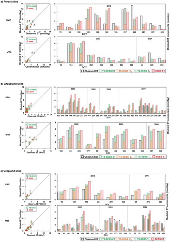
Figure 10. Taylor diagram shows the statistical comparison of modeled ET obtained from SEBS and TS-SEBS approaches in a) six selected sites, and b) land cover types

Seasonal variations of ET and T/ET

Figure 11 shows the time series of (a) precipitation and (b) ET from both SEBS approaches used in this study for the forest, grassland, and cropland sites, as well as (c) the EF ratio, which is critical to scale instantaneous LE to daily ET. Both SEBS models well-captured seasonal trends of daily ET compared with in-situ observations. Higher values were found during the growing season, and lower values were observed during the dormant season at the three ecosystem sites. Results of the time series showed that ET follows the seasonal trend of the year and results in larger ET followed by a precipitation event. This is natural since precipitation increases soil moisture, which evaporates at a potential rate, followed by a precipitation event resulting in a larger ET. For example, in the forest ecosystem of the SMC site, daily LE drastically increased after a rainfall event. This is because the SMC site is located over a thin soil layer, which has low retention of soil water content, for which monthly values range from 11% to 20% (Byun, Liaqat, and Choi 2014). Due to this low retention of soil water, most water after rainfall events are evaporated, which results in an increase in ET. Overall, better performances of both physical-based SEBS models used in this study are obvious due to the incorporation of medium-resolution TM/ETM+ satellite images and quality-controlled meteorological forcings (Liaqat and Choi 2015), which resulted in better flux estimations. However, temporal variations of TS-SEBS compared to SEBS showed almost equivalent daily ET across the time series at six sites, with the value of TS-SEBS being closer to in-situ observations. The ET obtained from the two SEBS approaches followed the temporal variations of EF in the six selected sites, which reveals that EF has a strong influence on estimating daily ET. We improved EF in our updated TS-SEBS model and estimated it separately for soil and canopy components. Therefore, the current improvement in daily ET by TS-SEBS is due to the implementation of improved formulations to estimate EF separately over soils and canopies, which resulted in better ET estimations. TS-SEBS showed better agreement than SEBS in reference to ground-based in-situ observations.

Figure 11. Time series analysis of precipitation, ET estimations from TS-SEBS and SEBS in comparison with corrected insitu ET, and EF as well as EF_S and EF_c are shown for two forest sites. Time series analysis of precipitation, ET estimations from TS-SEBS and SEBS in comparison with corrected insitu ET, and EF as well as EF_S and EF_C are shown for two grassland site. Time series analysis of precipitation, ET estimations from TS-SEBS and SEBS in comparison with corrected insitu ET, and EF as well as EF_S and EF_C are shown for two cropland site

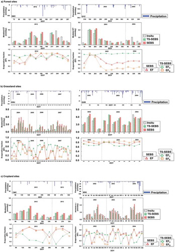
Since our study sites are located in subtropical, arid, and temperate zones, they receive a reasonable amount of precipitation during the monsoon season, which is the main driving force for ET. Such high values of ET during monsoon season are due to intercepted water at the top of the canopies along with an increase in soil moisture content after precipitation, which results in increase in transpiration and evaporation rates, respectively, with high incoming solar radiation (Hssaine et al. 2018; Tilahun 2006; Kurc and Small 2004). Overall, the ET values during the growing season were higher in lower latitudes of subtropical sites (such as QYZ) in comparison with the temperate zone of the SMC site due to the higher incoming solar radiation.

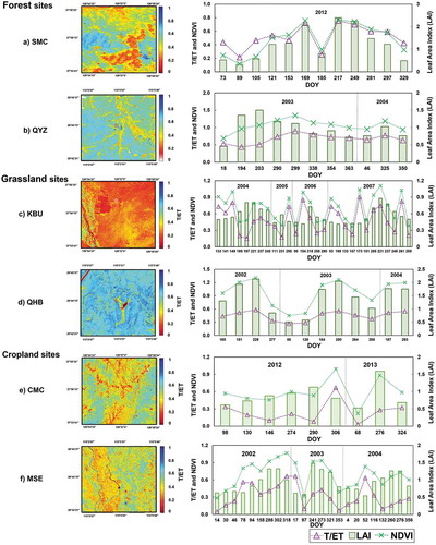
Figure 12 shows the spatial distribution and temporal variations of E/ET, which is key to assess stomatal response to environmental stresses and to predict hydrological cycles. Additionally, the relationships of T/ET with LAI and NDVI were analyzed. It is noteworthy that T/ET showed a linear relationship with LAI and NDVI because high LAI and NDVI result from high chlorophyll content, which produces a higher T and thus a higher T/ET ratio. The spatial distribution of T/ET in the six selected sites shows some regions with a T/ET ratio close to 0.2, which is attributed to a decrease in daily net radiation in those regions (Figure 14), in addition to the decreased vegetation health, temperature, and amount of precipitation in the winter for all selected sites.

Figure 12. Spatial variations of T/ET for growing season in sites: SMC (DOY = 153), QYZ (DOY = 203), KBU (DOY = 189), QHB (DOY = 181), CMC (DOY = 130), MSE (DOY = 158) are in left panel, whereas, the time series of T/ET at flux tower location are shown on right panel

Sensitivity analysis

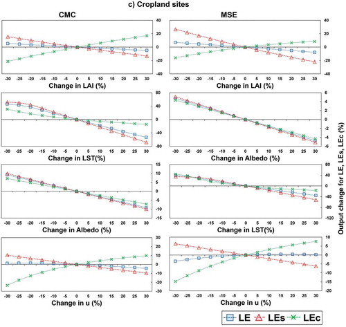
We conducted a detailed sensitivity analysis of TS-SEBS in SMC on DOY 153 (2012), QYZ on DOY 203 (2003), KBU on DOY 189 (2004), QHB on DOY 181 (2002), CMC on DOY 130 (2012), and MSE on DOY 158 (2002). We selected these dates because of their accurate ET estimation on those days, as demonstrated in Figure 9 and Figure 10. Here, we conducted a sensitivity analysis of LE, LE_S, and LE_C, and the results are presented in Figure 13a, 13b, and 13c for six selected sites in the forest, grassland, and cropland ecosystems, respectively. As shown, LST, albedo, and wind speed are all negatively correlated with LE, LE_S, and LE_C. Regarding LAI, the LE_S is negatively correlated, whereas LE and LE_C are positively correlated. The sensitivities of TS-SEBS from highest to lowest were as follows: LST<Albedo<LAI<wind speed, which reveals that a 10% increase in LST will result in a 15.9% decrease in LE, whereas a 10% increase in albedo will result in only a 2.88% decrease in LE. Similarly, a 10% increase in wind speed will result in only a 2.01% decrease in LE, which illustrates that albedo and wind speed have a little negative effect on estimated LE. A potential reason is that available energy and aerodynamic resistance are reduced with the corresponding increases in albedo and wind speed, resulting in a proportional decrease in LE. Additionally, LE_S is more sensitive to LAI, LST, and albedo compared with LE_C based on our sensitivity analysis. It is important to mention here that, since TS-SEBS uses LAI-based formulation to partition fluxes between soil and canopy components, the accurate quantification of LAI is vital to improve modeling results which may help to avoid propagation of uncertainties to energy flux components.

Figure 13. Sensitivity analysis of LAI, LST, Albedo and wind speed in two selected forest sites Sensitivity analysis of LAI, LST, Albedo and wind speed in two selected grassland sites Sensitivity analysis of LAI, LST, Albedo and wind speed in two selected cropland sites

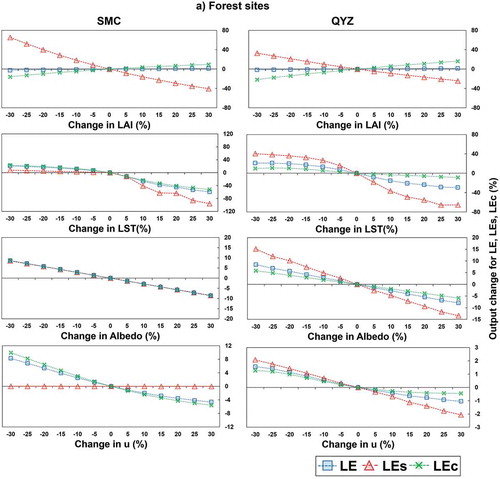
Figure 13. (Continued)

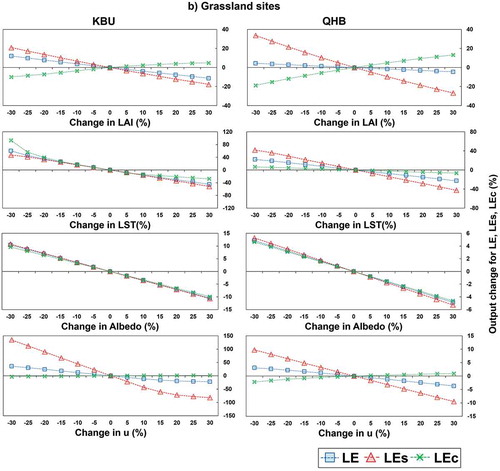
Figure 13. (Continued)

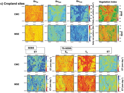
Spatially distributed mapping of improved evapotranspiration

Figure 14a, 14b, and 14c present spatially distributed mapping of daily radiation components (R_n24, R_n24S, and R_n24C), vegetation index (NDVI), ET, as well as its evaporation (E_S) component from soil and transpiration (T_C) components of the canopy at six selected sites for the forest, grassland, and cropland sites, respectively. The spatial distribution of R_n shows that the QYZ site receives more incoming daily solar radiation (~250 Wm⁻²) in most parts of the region compared with the SMC site. This is because the QYZ site is located at low latitude (in comparison with the SMC site) and receives greater incoming solar radiation in the high-sun season. Figure 14 shows delineated dashed rectangles, the inside of which reveals that the spatial distribution of the components of ET obtained from SEBS and TS-SEBS approaches closely follow the spatial distribution of radiation components. This is because incoming solar radiation is the main driving force for ET (Allen 1996). Moreover, due to its subtropical nature, the ET obtained from the QYZ site is higher, with a maximum value of ~9 mm day⁻¹ compared with ~6 mm day⁻¹ for the SMC site in the temperate zone. The ET obtained from TS-SEBS from inside the dashed rectangle in its QYZ site showed reduced ET values. The reason for this can be explained as follows. The dashed rectangles as presented for the QYZ site are low-elevation areas located between mountains and the canopy height of 13 m tends to cast a shadow in those areas due to aspect and slope factors, which significantly decrease the incoming solar radiation (Figure 14b). Thus, the ET obtained from those regions decreased. Overall, a comparison between the ET obtained from TS-SEBS and SEBS approaches demonstrates that both models adequately captured the seasonal trends, demonstrating the accuracy of our model.

Figure 14. Spatial mapping of radiation and ET components along with NDVI in two forest sites. Location of flux tower sites are indicated with stars. Spatial mapping of radiation and ET components along with NDVI in two grassland sites. Location of flux tower sites are indicated with stars. Spatial mapping of radiation and ET components along with NDVI in two cropland sites. Location of flux tower sites are indicated with stars

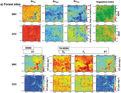
Figure 14. (Continued)

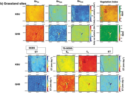
Figure 14. (Continued)

Conclusion

In this study, we developed a LAI-based formulation to convert a one-source Surface Energy Balance System (SEBS) to a two-source TS-SEBS model by exploiting reflectances and radiance information obtained from satellite earth observation datasets in combination with quality-controlled meteorological forcing datasets to estimate turbulent heat fluxes over soil and canopy components. We applied the updated TS-SEBS model using medium-resolution Landsat TM/ETM+ images for the period 2002–2013 at six selected sites corresponding to the forest, grassland, and cropland ecosystems in East Asia. The model estimations from TS-SEBS were independently compared with EC-based in-situ flux tower observations and with model estimations from single-source SEBS to provide a fair comparison and highlight the strength of our proposed model. The statistical metrics revealed that the mean estimated LE obtained from TS-SEBS was closer to the observed LE compared with that of SEBS. However, overestimation of LE was observed in an acceptable range, with mean bias values of 39.01 Wm⁻² for TS-SEBS and 57.96 Wm⁻² for SEBS in the six selected sites. The mean RMSE of ET obtained from TS-SEBS was reduced by ~13% compared to that of SEBS, revealing that TS-SEBS tends to show better ET approximations. Moreover, high computational efficiency, fewer input data requirements, and extended formulation to partition energy budget components between the canopy and soil components indicates TS-SEBS as a reliable alternative to water resource managers and the hydro-meteorological community for detailed land-plant-atmosphere interaction studies. The LAI-based formulations introduced in TS-SEBS to separately calculate EF, aerodynamic resistances, and introduction of an updated wind speed profile extinction coefficient results in TS-SEBS as a reliable alternative to SEBS. Overall, the TS-SEBS model proposed provides a benchmark study of partition energy budget components, opening new avenues for improved ET mapping and energy budget components by exploiting Landsat images at a local to regional scale.

Acknowledgements

This research was supported by the Basic Science Research Program through the National Research Foundation of Korea (NRF), funded by the Ministry of Education (NRF-2018R1D1A1B07049029). This work was supported by the National Research Foundation of Korea (NRF) grant funded by the Korea government (MSIT) (NRF-2019R1A2B5B01070196). This research was supported by the Higher Education Commission (HEC) of Pakistan government. This work used eddy covariance data acquired and shared by the FLUXNET community, including these networks: AmeriFlux, AfriFlux, AsiaFlux, ChinaFlux, KoFlux, LBA, NECC, OzFlux-TERN, TCOS-Siberia, and USCCC. The FLUXNET eddy covariance data processing and harmonization was carried out by the ICOS Ecosystem Thematic Center, AmeriFlux Management Project and Fluxdata project of FLUXNET, with the support of CDIAC, and the OzFlux, ChinaFlux and AsiaFlux offices. And, we also thank the Hydrological Survey Center (HSC), Republic of Korea, for providing unrestricted access to flux tower observations. We would like to thank the USGS for providing satellite images.

Disclosure statement

The authors declare that there is no conflict of interest in the context of this publication.

Additional information

Funding

This research was supported by the Basic Science Research Program through the National Research Foundation of Korea (NRF), funded by the Ministry of Education (NRF-2018R1D1A1B07049029). This work was supported by the National Research Foundation of Korea (NRF) grant funded by the Korea government (MSIT) (NRF-2019R1A2B5B01070196). This research was supported by the Higher Education Commission (HEC) of Pakistan government.

References

- Alfieri, J. G., W. P. Kustas, J. H. Prueger, L. E. Hipps, S. R. Evett, J. B. Basara, C. M. U. Neale, et al. 2012. “On the Discrepancy between Eddy Covariance and Lysimetry-based Surface Flux Measurements under Strongly Advective Conditions.” Advances in Water Resources 50 :62–78. doi:10.1016/j.advwatres.2012.07.008.
- Alkhaier, F., Z. Su, and G. N. Flerchinger. 2012. “Reconnoitering the Effect of Shallow Groundwater on Land Surface Temperature and Surface Energy Balance Using MODIS and SEBS.” Hydrology and Earth System Sciences 16 (7): 1833–1844. doi:10.5194/hess-16-1833-2012.
- Allen, R. 1996. “Assessing Integrity of Weather Data for Reference Evapotranspiration Estimation.” Journal of Irrigation and Drainage Engineering 122 (2): 2. doi:10.1061/(ASCE)0733-9437(1996)122:2(97).
- Allen, R., A. Irmak, R. Trezza, J. M. H. Hendrickx, W. Bastiaanssen, and J. Kjaersgaard. 2011. “Satellite-based ET Estimation in Agriculture Using SEBAL and METRIC.” Hydrological Processes 25 (26): 4011–4027. doi:10.1002/hyp.8408.
- Allen, R., M. Tasumi, and R. Trezza. 2007. “Satellite-Based Energy Balance for Mapping Evapotranspiration with Internalized Calibration (Metric)—model.” Journal of Irrigation and Drainage Engineering 133 (4): 380–394. doi:10.1061/(ASCE)0733-9437(2007)133:4(380).
- Anderson, M. C. 1997. “A Two-Source Time-Integrated Model for Estimating Surface Fluxes Using Thermal Infrared Remote Sensing.” Remote Sensing of Environment 60 (2): 195–216. doi:10.1016/S0034-4257(96)00215-5.
- Arnqvist, J., and H. Bergström. 2015. “Flux-profile Relation with Roughness Sublayer Correction.” Quarterly Journal of the Royal Meteorological Society 141 (689): 1191–1197. doi:10.1002/qj.2426.
- Badgley, G., J. B. Fisher, C. Jiménez, K. P. Tu, and R. Vinukollu. 2015. “On Uncertainty in Global Terrestrial Evapotranspiration Estimates from Choice of Input Forcing Datasets.” Journal of Hydrometeorology 16 (4): 1449–1455. doi:10.1175/jhm-d-14-0040.1.
- Bai, J., L. I. Jia, S. Liu, Z. Xu, G. Hu, M. Zhu, L. Song, et al. 2015. “Characterizing the Footprint of Eddy Covariance System and Large Aperture Scintillometer Measurements to Validate Satellite-Based Surface Fluxes.” IEEE Geoscience and Remote Sensing Letters 12 (5): 943–947. doi:10.1109/lgrs.2014.2368580.
- Bai, Y., X. Li, S. Zhou, X. Yang, K. Yu, M. Wang, S. Liu, et al. 2019. “Quantifying Plant Transpiration and Canopy Conductance Using Eddy Flux Data: An Underlying Water Use Efficiency Method.” Agricultural and Forest Meteorology 271 :375–384. doi:10.1016/j.agrformet.2019.02.035.
- Bastiaanssen, W. G. M., M. Menenti, R. A. Feddes, and A. A. M. Holtslag. 1998. “A Remote Sensing Surface Energy Balance Algorithm for Land (SEBAL). 1. Formulation.” Formulation. Journal of Hydrology 212-213: 198–212. doi:10.1016/S0022-1694(98)00253-4.
- Bhattarai, N., S. B. Shaw, L. J. Quackenbush, J. Im, and R. Niraula. 2016. “Evaluating Five Remote Sensing-Based Single-source Surface Energy Balance Models for Estimating Daily Evapotranspiration in a Humid Subtropical Climate.” International Journal of Applied Earth Observation and Geoinformation 49: 75–86. doi:10.1016/j.jag.2016.01.010.
- Bisquert, M., J. M. Sánchez, R. López-Urrea, and V. Caselles. 2016. “Estimating High Resolution Evapotranspiration from Disaggregated Thermal Images.” Remote Sensing of Environment 187: 423–433. doi:10.1016/j.rse.2016.10.049.
- Brutsaert, W. 1999. “Aspects of Bulk Atmospheric Boundary Layer Similarity under Free-convective Conditions.” Reviews of Geophysics 37 (4): 439–451. doi:10.1029/1999rg900013.
- Brutsaert, W. 2005. Hydrology: An Introduction. New York, NY: Cambridge University Press. ISBN: 9780521824798 doi.10.1017/CBO9780511808470.
- Burchard- Levine, Vicente, Héctor Nieto, David Riaño, Mirco Migliavacca, Tarek S. El-Madany, Oscar Perez-Priego, Arnaud Carrara, and M. Pilar Martín. 2019. “Adapting the thermal-based two-source energy balance model to estimate energy fluxes in a complex tree-grass ecosystem..” Hydrology and Earth System Sciences Discussions org/10.5194/hess-2019-354.
- Byun, K., U. W. Liaqat, and M. Choi. 2014. “Dual-model Approaches for Evapotranspiration Analyses over Homo- and Heterogeneous Land Surface Conditions.” Agricultural and Forest Meteorology 197: 169–187. doi:10.1016/j.agrformet.2014.07.001.
- Cammalleri, C., G. Rallo, C. Agnese, G. Ciraolo, M. Minacapilli, and G. Provenzano. 2013. “Combined Use of Eddy Covariance and Sap Flow Techniques for Partition of ET Fluxes and Water Stress Assessment in an Irrigated Olive Orchard.” Agricultural Water Management 120 :89–97. doi:10.1016/j.agwat.2012.10.003.
- Chen, J. M., and J. Liu. 2020. “Evolution of Evapotranspiration Models Using Thermal and Shortwave Remote Sensing Data.” Remote Sensing of Environment 237: 111594. doi:10.1016/j.rse.2019.111594.
- Chen, X., Z. Su, Y. Ma, and E. M. Middleton. 2019. “Optimization of a Remote Sensing Energy Balance Method over Different Canopy Applied at Global Scale.” Agricultural and Forest Meteorology 279: 107633. doi:10.1016/j.agrformet.2019.107633.
- Chen, X., Z. Su, Y. Ma, K. Yang, J. Wen, and Y. Zhang. 2013. “An Improvement of Roughness Height Parameterization of the Surface Energy Balance System (SEBS) over the Tibetan Plateau.” Journal of Applied Meteorology and Climatology 52 (3): 607–622. doi:10.1175/jamc-d-12-056.1.
- Chen, X., Z. Su, Y. Ma, S. Liu, Q. Yu, and Z. Xu. 2014. “Development of a 10-year (2001–2010) 0.1° Data Set of Land-surface Energy Balance for Mainland China.” Atmospheric Chemistry and Physics 14 (23): 13097–13117. doi:10.5194/acp-14-13097-2014.
- Cook, D. R., and R. C. Sullivan, 2019. “Energy Balance Bowen Ratio (EBBR) Instrument Handbook”. United States. USDOE Office of Environmental Management. In: Energy, U.D.o. (Ed.). DOI:10.2172/1020562
- Crago, R., and W. Brutsaert. 1996. “Daytime Evaporation and the Self-preservation of the Evaporative Fraction and the Bowen Ratio.” Journal of Hydrology 178 (1–4): 241–255. doi:10.1016/0022-1694(95)02803-X.
- Deguchi, A., S. Hattori, and H.-T. Park. 2006. “The Influence of Seasonal Changes in Canopy Structure on Interception Loss: Application of the Revised Gash Model.” Journal of Hydrology 318 (1–4): 80–102. doi:10.1016/j.jhydrol.2005.06.005.
- Ershadi, A., M. McCabe, J. P. Evans, and J. P. Walker. 2013. “Effects of Spatial Aggregation on the Multi-scale Estimation of Evapotranspiration.” Remote Sensing of Environment 131: 51–62. doi:10.1016/j.rse.2012.12.007.
- Farah, H. O., W. G. M. Bastiaanssen, and R. A. Feddes. 2004. “Evaluation of the Temporal Variability of the Evaporative Fraction in a Tropical Watershed.” International Journal of Applied Earth Observation and Geoinformation 5 (2): 129–140. doi:10.1016/j.jag.2004.01.003.
- Fisher, J. B., F. Melton, E. Middleton, C. Hain, M. Anderson, R. Allen, M. F. McCabe, et al. 2017. “The Future of Evapotranspiration: Global Requirements for Ecosystem Functioning, Carbon and Climate Feedbacks, Agricultural Management, and Water Resources.” Water Resources Research 53 (4): 2618–2626. doi:10.1002/2016WR020175.
- Gibson, L., Z. Munch, and J. Engelbrecht. 2011. “Particular Uncertainties Encountered in Using a Pre-packaged SEBS Model to Derive Evapotranspiration in a Heterogeneous Study Area in South Africa.” Hydrology and Earth System Sciences 15 (1): 295–310. doi:10.5194/hess-15-295-2011.
- Gokmen, M., Z. Vekerdy, A. Verhoef, W. Verhoef, O. Batelaan, and C. van der Tol. 2012. “Integration of Soil Moisture in SEBS for Improving Evapotranspiration Estimation under Water Stress Conditions.” Remote Sensing of Environment 121 :261–274. doi:10.1016/j.rse.2012.02.003.
- Gowda, P. H., J. L. Chavez, P. D. Colaizzi, S. R. Evett, T. A. Howell, and J. A. Tolk. 2008. “ET Mapping for Agricultural Water Management: Present Status and Challenges.” Irrigation Science 26 (3): 223–237. doi:10.1007/s00271-007-0088-6.
- Gowda, P. H., T. A. Howell, G. Paul, P. D. Colaizzi, T. H. Marek, B. Su, K. S. Copeland et al. 2013. “Deriving Hourly Evapotranspiration Rates with SEBS: A Lysimetric Evaluation.” Vadose Zone Journal 12 (3): 3. DOI:10.2136/vzj2012.0110.
- Hess, A., B. Wadzuk, and A. Welker. 2017. “Evapotranspiration in Rain Gardens Using Weighing Lysimeters.” Journal of Irrigation and Drainage Engineering 143 (6): 04017004. doi:10.1061/(ASCE)IR.1943-4774.0001157.
- Hsieh, C.-I., G. Katul, and T.-W. Chi. 2000. “An Approximate Analytical Model for Footprint Estimation of Scalar fluxes in Thermally stratified Atmospheric flows.” Advances in Water Resources 23 (7): 765–772. doi:10.1016/S0309-1708(99)00042-1.
- Hssaine, B. A., O. Merlin, Z. Rafi, J. Ezzahar, L. Jarlan, S. Khabba, S. Er-Raki, et al. 2018. “Calibrating an Evapotranspiration Model Using Radiometric Surface Temperature, Vegetation Cover Fraction and Near-surface Soil Moisture Data.” Agricultural and Forest Meteorology 256-257 :104–115. doi:10.1016/j.agrformet.2018.02.033.
- Huang, C., Y. Li, J. Gu, L. Lu, and X. Li. 2015. “Improving Estimation of Evapotranspiration under Water-Limited Conditions Based on SEBS and MODIS Data in Arid Regions.” Remote Sensing 7 (12): 16795–16814. doi:10.3390/rs71215854.
- Janssen, T., K. Fleischer, S. Luyssaert, K. Naudts, and H. Dolman. 2020. “Drought Resistance Increases from the Individual to the Ecosystem Level in Highly Diverse Neotropical Rainforest: A Meta-analysis of Leaf, Tree and Ecosystem Responses to Drought.” Biogeosciences 17 (9): 2621–2645. doi:10.5194/bg-17-2621-2020.
- Jia, L., G. Xi, S. Liu, C. Huang, Y. Yan, and G. Liu. 2009. “Regional Estimation of Daily to Annual Regional Evapotranspiration with MODIS Data in the Yellow River Delta Wetland.” Hydrology and Earth System Sciences 13 (10): 1775–1787. DOI:10.5194/hess-13-1775-2009.
- Jia, Z., S. Liu, Z. Xu, Y. Chen, and M. Zhu. 2012. “Validation of Remotely Sensed Evapotranspiration over the Hai River Basin, China”. Journal of Geophysical Research: Atmospheres 117(D13). (D13):n/a-n/a. doi:10.1029/2011jd017037.
- Jung, M., M. Reichstein, P. Ciais, S. I. Seneviratne, J. Sheffield, M. L. Goulden, G. Bonan, et al. 2010. “Recent Decline in the Global Land Evapotranspiration Trend Due to Limited Moisture Supply.” Nature 467 (7318): 951–954. doi:10.1038/nature09396.
- Khan, M. S., U. W. Liaqat, J. Baik, M. Choi. 2018. “Stand-alone uncertainty characterization of GLEAM, GLDAS and MOD16 evapotranspiration products using an extended triple collocation approach..”Agricultural and Forest Meteorology 252 : 256–268.org/10.1016/j.agrformet.2018.01.022.
- Khan, M. S., Baik M. Choi. 2020. Inter-comparison of evapotranspiration datasets over heterogeneous landscapes across Australia.“Advances in Space Research” 66 no. 3: 533–545. org/10.1016/j.asr.2020.04.037.
- Konings, A. G., A. P. Williams, and P. Gentine. 2017. “Sensitivity of Grassland Productivity to Aridity Controlled by Stomatal and Xylem Regulation.” Nature Geoscience 10 (4): 284–288. doi:10.1038/ngeo2903.
- Kool, D., N. Agam, N. Lazarovitch, J. L. Heitman, T. J. Sauer, and A. Ben-Gal. 2014. “A Review of Approaches for Evapotranspiration Partitioning.” Agricultural and Forest Meteorology 184 :56–70. doi:10.1016/j.agrformet.2013.09.003.
- Kurc, S. A., and E. E. Small. 2004. “Dynamics of Evapotranspiration in Semiarid Grassland and Shrubland Ecosystems during the Summer Monsoon Season, Central New Mexico.” Water Resources Research 40 (9): 9. doi:10.1029/2004wr003068.
- Kustas, W. P., C. S. T. Daughtry, and P. J. V. Oevelen. 1993. “Analytical Treatment of the Relationships between Soil Heat Flux/Net Radiation Ratio and Vegetation Indices.” Remote Sensing of Environment 46 (3): 319–330. 10.1016/0034-4257(93)90052-Y
- Kustas, W. P., and C. S. T. Daughtry. 1990. “Estimation of the Soil Heat Flux/net Radiation Ratio from Spectral Data.” Agricultural and Forest Meteorology 49 (3): 205–223. doi:10.1016/0168-1923(90)90033-3.
- Kustas, W. P., and J. M. Norman. 1999a. “Evaluation of Soil and Vegetation Heat Flux Predictions Using a Simple Two-source Model with Radiometric Temperatures for Partial Canopy Cover.” Agricultural and Forest Meteorology 94: 13–29. doi.org/10.1016/S0168-1923(99)00005-2.
- Kustas, W. P., and J. M. Norman. 1999b. “Reply to Comments about the Basic Equations of Dual-source Vegetation–atmosphere Transfer Models.” Agricultural and Forest Meteorology 94 (3–4): 275–278. doi:10.1016/S0168-1923(99)00012-X.
- Kustas, W. P., K. S. Humes, J. M. Norman, and M. S. Moran. 1996. “Single- and Dual-Source Modeling of Surface Energy Fluxes with Radiometric Surface Temperature.” Journal of Applied Meteorology 35 (1): 110–121. doi:10.1175/1520-0450(1996)035<0110:SADSMO>2.0.CO;2.
- Kwon, H., J.-H. Lee, Y.-K. Lee, J.-W. Lee, S.-W. Jung, and J. Kim. 2009. “Seasonal Variations of Evapotranspiration Observed in a Mixed Forest in the Seolmacheon Catchment.” Korean Journal of Agricultural and Forest Meteorology 11 (1): 39–47. doi:10.5532/KJAFM.2009.11.1.039.
- Lang, D., J. Zheng, J. Shi, F. Liao, X. Ma, W. Wang, X. Chen, et al. 2017. “A Comparative Study of Potential Evapotranspiration Estimation by Eight Methods with FAO Penman–Monteith Method in Southwestern China.” Water 9 (10): 10. doi:10.3390/w9100734.
- Lee, D., J. Kim, K.-S. Lee, and S. Kim. 2010. “Partitioning of Catchment Water Budget and Its Implications for Ecosystem Carbon Exchange.” Biogeosciences 7 (6): 1903–1914. doi:10.5194/bg-7-1903-2010.
- Legates, D. R., and G. J. McCabe. 1999. “Evaluating the Use of “Goodness-of-fit” Measures in Hydrologic and Hydroclimatic Model Validation.” Water Resources Research 35 (1): 233–241. doi:10.1029/1998wr900018.
- Li, F., W. P. Kustas, J. H. Prueger, C. M. U. Neale, and T. J. Jackson. 2005. “Utility of Remote Sensing–Based Two-Source Energy Balance Model under Low- and High-Vegetation Cover Conditions.” Journal of Hydrometeorology 6: 878–891. doi.org/10.1175/JHM464.1.
- Li, X., P. Gentine, C. Lin, S. Zhou, Z. Sun, Y. Zheng, J. Liu, et al. 2019. “A Simple and Objective Method to Partition Evapotranspiration into Transpiration and Evaporation at Eddy-covariance Sites.” Agricultural and Forest Meteorology 265 :171–182. doi:10.1016/j.agrformet.2018.11.017.
- Li, Y., C. Huang, J. Hou, J. Gu, G. Zhu, and X. Li. 2017. “Mapping Daily Evapotranspiration Based on Spatiotemporal Fusion of ASTER and MODIS Images over Irrigated Agricultural Areas in the Heihe River Basin, Northwest China.” Agricultural and Forest Meteorology 244-245 :82–97. doi:10.1016/j.agrformet.2017.05.023.
- Li, Y., J. Zhou, H. Wang, D. Li, R. Jin, Y. Zhou, Q. Zhou, et al. 2015. “Integrating Soil Moisture Retrieved from L-band Microwave Radiation into an Energy Balance Model to Improve Evapotranspiration Estimation on the Irrigated Oases of Arid Regions in Northwest China.” Agricultural and Forest Meteorology 214-215 :306–318. doi:10.1016/j.agrformet.2015.08.260.
- Liaqat, U. W., and M. Choi. 2015. “Surface Energy Fluxes in the Northeast Asia Ecosystem: SEBS and METRIC Models Using Landsat Satellite Images.” Agricultural and Forest Meteorology 214-215: 60–79. doi:10.1016/j.agrformet.2015.08.245.
- Liaqat, U. W., and M. Choi. 2017. “Accuracy Comparison of Remotely Sensed Evapotranspiration Products and Their Associated Water Stress Footprints under Different Land Cover Types in Korean Peninsula.” Journal of Cleaner Production 155: 93–104. doi:10.1016/j.jclepro.2016.09.022.
- Long, D., and V. P. Singh. 2012a. “A Modified Surface Energy Balance Algorithm for Land (M-SEBAL) Based on A Trapezoidal Framework.” Water Resources Research 48 (2): 2. doi:10.1029/2011wr010607.
- Long, D., and V. P. Singh. 2012b. “A Two-source Trapezoid Model for Evapotranspiration (TTME) from Satellite Imagery.” Remote Sensing of Environment 121: 370–388. doi:10.1016/j.rse.2012.02.015.
- Lu, J., Z.-L. Li, R. Tang, B.-H. Tang, H. Wu, F. Yang, J. Labed, et al. 2012. “Evaluating the SEBS-estimated Evaporative Fraction from MODIS Data for a Complex Underlying Surface.” Hydrological Processes: N/a-n/a. doi:10.1002/hyp.9440.
- Ma, W., Z. Wei, P. Wang, and J. Asanuma. 2020. “Transpiration and Evaporation of Grassland Using Land Surface modelling.” Hydrological Processes 34 (17): 3656–3668. doi:10.1002/hyp.13792.
- Ma, Y., S. Liu, L. Song, Z. Xu, Y. Liu, T. Xu, Z. Zhu, et al. 2018. “Estimation of Daily Evapotranspiration and Irrigation Water Efficiency at a Landsat-like Scale for an Arid Irrigation Area Using Multi-source Remote Sensing Data.” Remote Sensing of Environment 216 :715–734. doi:10.1016/j.rse.2018.07.019.
- Marshall, M., P. Thenkabail, T. Biggs, and K. Post. 2016. “Hyperspectral Narrowband and Multispectral Broadband Indices for Remote Sensing of Crop Evapotranspiration and Its Components (Transpiration and Soil Evaporation).” Agricultural and Forest Meteorology 218-219: 122–134. doi:10.1016/j.agrformet.2015.12.025.
- Massman, W. J. 1996. “An Analytical One-Dimensional Model of Momentum Transfer by Vegetation of Arbitrary Structure.” Boundary-Layer Meteorology 83 (3): 407–421. doi:10.1023/A:1000234813011.
- Massman, W. J., J. M. Forthofer, and M. A. Finney. 2017. “An Improved Canopy Wind Model for Predicting Wind Adjustment Factors and Wildland Fire Behavior.” Canadian Journal of Forest Research 47 (5): 594–603. doi:10.1139/cjfr-2016-0354.
- Mastrotheodoros, T., C. Pappas, P. Molnar, P. Burlando, T. F. Keenan, P. Gentine, C. M. Gough, and S. Fatichi. 2017. “Linking Plant Functional Trait Plasticity and the Large Increase in Forest Water Use Efficiency.” Journal of Geophysical Research: Biogeosciences 122 (9): 2393–2408. doi:10.1002/2017jg003890.
- Mecikalski, J. R., G. R. Diak, M. C. Anderson, and J. M. Norman. 1999. “Estimating Fluxes on Continental Scales Using Remotely Sensed Data in an Atmospheric–Land Exchange Model.” Journal of Applied Meteorology 38 (9): 1352–1369. doi:10.1175/1520-0450(1999)038<1352:EFOCSU>2.0.CO;2.
- Michel, D., C. Jiménez, D. G. Miralles, M. Jung, M. Hirschi, A. Ershadi, B. Martens et al. 2016. “The WACMOS-ET Project – Part 1: Tower-scale Evaluation of Four Remote-sensing-based Evapotranspiration Algorithms.” Hydrology and Earth System Sciences 20 (2): 803–822. DOI:10.5194/hess-20-803-2016.
- Miralles, D. G., C. Jiménez, M. Jung, D. Michel, A. Ershadi, M. F. McCabe, M. Hirschi et al. 2016. “The WACMOS-ET project – Part 2: Evaluation of Global Terrestrial Evaporation Data Sets.” Hydrology and Earth System Sciences 20 (2): 823–842. DOI:10.5194/hess-20-823-2016.
- Miralles, D. G., P. Gentine, S. I. Seneviratne, and A. J. Teuling. 2019. “Land-atmospheric Feedbacks during Droughts and Heatwaves: State of the Science and Current Challenges.” Annals of the New York Academy of Sciences 1436 (1): 19. doi:10.1111/nyas.13912.
- Miralles, D. G., T. R. H. Holmes, R. A. M. De Jeu, J. H. Gash, A. G. C. A. Meesters, and A. J. Dolman. 2011. “Global Land-surface Evaporation Estimated from Satellite-based Observations.” Hydrology and Earth System Sciences 15 (2): 453–469. doi:10.5194/hess-15-453-2011.
- Monin, A. S., and A. M. L. Obukhov. 1954. “Basic Laws of Turbulent Mixing in the Surface Layer of the Atmosphere.” Contrib. Geophys. Inst. Acad. Sci. USSR 151 (163): e187.
- Montoro, A., F. Mañas, and R. López-Urrea. 2016. “Transpiration and Evaporation of Grapevine, Two Components Related to Irrigation Strategy.” Agricultural Water Management 177: 193–200. doi:10.1016/j.agwat.2016.07.005.
- Mu, Q., M. Zhao, and S. Running. 2011. “MODIS Global Evapotranspiration Project (MOD16)”. NASA/EOS
- Norman, J. M., W. P. Kustas, J. H. Prueger, and G. R. Diak. 2000. “Surface Flux Estimation Using Radiometric Temperature: A Dual-temperature-difference Method to Minimize Measurement Errors.” Water Resources Research 36 (8): 2263–2274. doi:10.1029/2000wr900033.
- Norman, J. M., W. P. Kustas, and K. S. Humes. 1995. “Source Approach for Estimating Soil and Vegetation Energy Fluxes in Observations of Directional Radiometric Surface Temperature.” Agricultural and Forest Meteorology 77 (3–4): 263–293. doi:10.1016/0168-1923(95)02265-Y.
- Pradhan, R., N. Singh, and R. P. Singh. 2019. “Onset of Summer Monsoon in Northeast India Is Preceded by Enhanced Transpiration.” Scientific Reports 9 (1): 18646. doi:10.1038/s41598-019-55186-8.
- Purdy, A. J., J. B. Fisher, M. L. Goulden, and J. S. Famiglietti. 2016. “Ground Heat Flux: An Analytical Review of 6 Models Evaluated at 88 Sites and Globally.” Journal of Geophysical Research: Biogeosciences 121 (12): 3045–3059. doi:10.1002/2016jg003591.
- Qin, Z., A. Karnieli, and P. Berliner. 2001. “A Mono-window Algorithm for Retrieving Land Surface Temperature from Landsat TM Data and Its Application to the Israel-Egypt Border Region.” International Journal of Remote Sensing 22 (18): 3719–3746. doi:10.1080/01431160010006971.
- Rahman, M. M., and W. Zhang. 2019. “Validation of Satellite-Derived Sensible Heat Flux for TERRA/MODIS Images over Three Different Landscapes Using Large Aperture Scintillometer and Eddy Covariance Measurements.” IEEE Journal of Selected Topics in Applied Earth Observations and Remote Sensing 12 (9): 3327–3337. doi:10.1109/jstars.2019.2928880.
- Rigden, A. J., and G. D. Salvucci. 2017. “Stomatal Response to Humidity and CO 2 Implicated in Recent Decline in US Evaporation.” Global Change Biology 23 (3): 1140–1151. doi:10.1111/gcb.13439.
- Sánchez, J. M., W. P. Kustas, V. Caselles, and M. C. Anderson. 2008. “Modelling Surface Energy Fluxes over Maize Using a Two-source Patch Model and Radiometric Soil and Canopy Temperature Observations.” Remote Sensing of Environment 112 (3): 1130–1143. doi:10.1016/j.rse.2007.07.018.
- Song, L., Z. Bian, W. P. Kustas, S. Liu, Q. Xiao, H. Nieto, Z. Xu, et al. 2020. “Estimation of Surface Heat Fluxes Using Multi-angular Observations of Radiative Surface Temperature.” Remote Sensing of Environment 239 :111674. doi:10.1016/j.rse.2020.111674.
- Su, Z. 2002. “The Surface Energy Balance System (SEBS) for Estimation of Turbulent Heat Fluxes.” Hydrology and Earth System Sciences 6 (1): 85–99. doi:10.5194/hess-6-85-2002.
- Su, Z. B. 2001. A Surface Energy Balance System (SEBS) for Estimation of Turbulent Heat Fluxes from Point to Continental Scale. Spectra Workshop. Publications of the National Remote Sensing Board (BCRS), USP-2: 01-02.
- Talsma, C. J., S. P. Good, C. Jimenez, B. Martens, J. B. Fisher, D. G. Miralles, M. F. McCabe, et al. 2018. “Partitioning of Evapotranspiration in Remote Sensing-based Models.” Agricultural and Forest Meteorology 260-261 :131–143. doi:10.1016/j.agrformet.2018.05.010.
- Tasumi, M., R. Allen, and R. Trezza. 2008. “At-Surface Reflectance and Albedo from Satellite for Operational Calculation of Land Surface Energy Balance.” Journal of Hydrologic Engineering 13 (2): 51–63. doi:10.1061/(ASCE)1084-0699(2008)13:2(51).
- Taylor, G. I., 1938. “The Spectrum of Turbulence”. Proceedings of the Royal Society of London. Series A-Mathematical and Physical Sciences, 164( 919): 476–490.
- Taylor, K. E. 2001. “Summarizing Multiple Aspects of Model Performance in a Single Diagram.” Journal of Geophysical Research: Atmospheres 106 (D7): 7183–7192. doi:10.1029/2000jd900719.
- Tilahun, K. 2006. “Analysis of Rainfall Climate and Evapo-transpiration in Arid and Semi-arid Regions of Ethiopia Using Data over the Last Half a Century.” Journal of Arid Environments 64 (3): 474–487. doi:10.1016/j.jaridenv.2005.06.013.
- Timmermans, J., Z. Su, C. V. D. Tol, A. Verhoef, and W. Verhoef. 2013. “Quantifying the Uncertainty in Estimates of Surface–atmosphere Fluxes through Joint Evaluation of the SEBS and SCOPE Models.” Hydrology and Earth System Sciences 17 (4): 1561–1573. doi:10.5194/hess-17-1561-2013.
- Trezza, R., R. Allen, and M. Tasumi. 2013. “Estimation of Actual Evapotranspiration along the Middle Rio Grande of New Mexico Using MODIS and Landsat Imagery with the METRIC Model.” Remote Sensing 5 (10): 5397–5423. doi:10.3390/rs5105397.
- Twine, T. E., W. P. Kustas, J. M. Norman, D. R. Cook, P. R. Houser, T. P. Meyers, J. H. Prueger et al. 2000. “Correcting Eddy-covariance Flux Underestimates over a Grassland.” Agricultural and Forest Meteorology 103 (3): 279–300. DOI:10.1016/S0168-1923(00)00123-4.
- Wang, Y., X. Li, and S. Tang. 2013. “Validation of the SEBS-derived Sensible Heat for FY3A/VIRR and TERRA/MODIS over an Alpine Grass Region Using LAS Measurements.” International Journal of Applied Earth Observation and Geoinformation 23: 226–233. doi:10.1016/j.jag.2012.09.005.
- Webster, E., D. Ramp, and R. T. Kingsford. 2017. “Incorporating an Iterative Energy Restraint for the Surface Energy Balance System (SEBS).” Remote Sensing of Environment 198: 267–285. doi:10.1016/j.rse.2017.06.012.
- Xue, J., K. M. Bali, S. Light, T. Hessels, and I. Kisekka. 2020. “Evaluation of Remote Sensing-based Evapotranspiration Models against Surface Renewal in Almonds.” Tomatoes and Maize. Agricultural Water Management 238. doi:10.1016/j.agwat.2020.106228.
- Yang, X., B. Yong, L. Ren, Y. Zhang, and D. Long. 2017. “Multi-scale Validation of GLEAM Evapotranspiration Products over China via ChinaFLUX ET Measurements.” International Journal of Remote Sensing 38 (20): 5688–5709. doi:10.1080/01431161.2017.1346400.
- Yang, Y., M. Anderson, F. Gao, C. Hain, A. Noormets, G. Sun, R. Wynne, V. Thomas, and L. Sun. 2018a. “Investigating Impacts of Drought and Disturbance on Evapotranspiration over a Forested Landscape in North Carolina, USA Using High Spatiotemporal Resolution Remotely Sensed Data.” Remote Sensing of Environment. doi:10.1016/j.rse.2018.12.017.
- Yang, Y., H. Su, R. Zhang, J. Tian, and L. Li. 2015. “An Enhanced Two-source Evapotranspiration Model for Land (ETEML): Algorithm and Evaluation.” Remote Sensing of Environment 168: 54–65. doi:10.1016/j.rse.2015.06.020.
- Yang, Y., J. Qiu, R. Zhang, S. Huang, S. Chen, H. Wang, J. Luo, et al. 2018b. “Intercomparison of Three Two-Source Energy Balance Models for Partitioning Evaporation and Transpiration in Semiarid Climates.” Remote Sensing 10 (7): 7. doi:10.3390/rs10071149.
- Yang, Y., and S. Shang. 2013. “A Hybrid Dual-source Scheme and Trapezoid Framework-based Evapotranspiration Model (HTEM) Using Satellite Images: Algorithm and Model Test.” Journal of Geophysical Research: Atmospheres 118 (5): 2284–2300. doi:10.1002/jgrd.50259.
- Yao, Y., S. Liang, J. Yu, J. Chen, S. Liu, Y. Lin, J.B. Fisher, T.R. McVicar, J. Cheng, K. Jia, and X. Zhang. 2017. “A Simple Temperature Domain Two-source Model for Estimating Agricultural Field Surface Energy Fluxes from Landsat Images.” Journal of Geophysical Research: Atmospheres 122 (10): 5211–5236. doi:10.1002/2016jd026370.
- Yu, B., S. Shang, W. Zhu, P. Gentine, and Y. Cheng. 2019. “Mapping Daily Evapotranspiration over a Large Irrigation District from MODIS Data Using a Novel Hybrid Dual-source Coupling Model.” Agricultural and Forest Meteorology 276-277: 107612. doi:10.1016/j.agrformet.2019.06.011.
- Zhang, S., H. Chen, Y. Fu, H. Niu, Y. Yang, and B. Zhanget. 2019. “Fractional Vegetation Cover Estimation of Different Vegetation Types in the Qaidam Basin.” Sustainability 11 :3. doi:10.3390/su11030864.
- Zhao, J., X. Chen, J. Zhang, H. Zhao, and Y. Song. 2019. “Higher Temporal Evapotranspiration Estimation with Improved SEBS Model from Geostationary Meteorological Satellite Data.” Scientific Reports 9 (1): 14981. doi:10.1038/s41598-019-50724-w.
- Zhao, T., W. Zhang, Y. Zhang, Z. Liu, and X. Chen. 2020. “Significant Spatial Patterns from the GCM Seasonal Forecasts of Global Precipitation.” Hydrology and Earth System Sciences 24 (1): 1–16. doi:10.5194/hess-24-1-2020.