The impact of voxel size, forest type, and understory cover on visibility estimation in forests using terrestrial laser scanning

ABSTRACT

Visibility (or viewshed) analysis, a common function in geographical information systems, is used in a wide range of fields such as urban planning, landscape management, and ecological research. However, measuring fine-scale visibility within a forest environment is challenging due to the structural complexity of plant architecture. Here we propose a new method for estimating visibility in forests using terrestrial laser scanning (TLS). We compare the visibility in forest plots derived from TLS with that derived from the gold standard photography-based approach and show that there is good agreement between the visibility derived from TLS-based and photography-based approaches with $R^2$ values ranging from 0.67 to 0.79 and RMSE values ranging from 12.45% to 17.29%. We further examine the potential impacts of voxel size, forest type, and understory cover on TLS-based estimation accuracy. Voxel size has a strong effect on visibility estimates, with the most accurate estimates obtained at a voxel size of 10 cm. In general, the TLS-based approach achieves higher estimation accuracy in deciduous forest plots than in coniferous and mixed forest plots. The understory has a significant effect on the estimates, with a lower accuracy for dense understory cover. Our results demonstrate that TLS technology can serve as an appropriate approach to rapidly estimate fine-scale visibility in forests. More importantly, TLS provides the opportunity to move beyond estimating visibility at single locations and from limited perspectives, to estimating visibility at any location and from any perspective within a scanned area, thereby greatly improving sampling efficiency.

KEYWORDS:

• Voxel size
• forest type
• understory
• viewshed
• terrestrial LiDAR

1. Introduction

Visibility (or viewshed) analysis is a common function of almost all geographic information systems (GIS) and has been used in many disciplines. For example, visibility analysis has been extensively used to examine and evaluate architectural design and built-up configurations in urban space (Benedikt 1979; Batty 2001). The visual character and impact of roadways through scenic areas were assessed by evaluating landscape visual quality (Martín et al. 2016). Target detection and the view under a canopy in forest landscapes have been modeled using military GIS software (Stanford et al. 2003; Caldwell, Ehlen, and Harmon 2005). Loarie, Tambling, and Asner (2013) quantified visibility where lion (Panthera leo) kills occurred in an African savanna and found significant differences in the type of vegetation used by male and female lions during hunts. Kuijper et al. (2014) studied whether perceived predation risk in red deer (Cervus elaphus) and wild boar (Sus scrofa) is related to habitat visibility in dense forest. However, despite the successful application of visibility analysis in the above-mentioned fields, previous work indicates that measuring fine-scale visibility within a forest environment is challenging due to the structural complexity of plant architecture (Murgoitio et al. 2014).

Visibility estimation is usually achieved by testing if the line of sight between the observer and the target is obstructed (Liu et al. 2008). Therefore, a fundamental question in line-of-sight analysis is how to represent an environmental scene using a digital model (Hagstrom et al. 2011). Most existing line-of-sight analysis methods are implemented using a surface scene model. These surface models are robust over large-scale areas where the line of sight is mainly affected by large objects. However, they no longer yield good approximations in smaller areas of interest containing detailed objects and complex scene geometry (Hagstrom et al. 2011).

Environmental components such as vegetation, terrain, and artificial infrastructure all affect the visibility of the surrounding area across spatial scales. For forests in particular, how vegetation is represented has an impact on how visibility is perceived at different spatial scales. For long-range visibility estimation that encompasses many kilometers, visual obstruction is dominated by terrain (Vukomanovic et al. 2018), so visibility is usually estimated by using a digital elevation model (DEM) where vegetation is treated as a continuous and opaque surface draped on the terrain (Seixas, Mediano, and Gattass 1999; Loarie, Tambling, and Asner 2013). For close-range visibility estimation ranging from several hundred meters to a few kilometers, vegetation may have a significant impact on visibility (Murgoitio et al. 2013). Some studies have used regular geometric shapes and inserted these artificial “trees” into a DEM on which visibility analysis was executed (Stanford et al. 2003; Liu et al. 2008). Some other studies have incorporated vegetation into visibility models using visual permeability (Dean 1997; Llobera 2007). In these studies, tree obstructions have been treated as solid structures. For some applications, such as animal ecological studies and military purposes, visibility needs to be estimated at ranges from several to dozens of meters where the view is often lateral and underneath a canopy. At this very short range and especially in regions with high vegetation density, visual obstruction is often dominated by fine-scale three-dimensional (3D) vegetation structure including trunks, branches, leaves, and internal gaps. Murgoitio et al. (2013) used tree height and diameter at breast height to incorporate tree trunks as obstructions into the visibility model, but branches and leaves were ignored. Because of the inability of digital surfaces to factor detailed 3D vegetation structure into visibility modeling, approaches used to measure fine-scale visibility in forests are currently field-based, with visibility generally estimated by determining the percentage to which a distant reference object of known dimensions is being covered by vegetation from a given vantage point (Higgins et al. 1996).

The two most common reference objects used in traditional field-based visibility analysis are a cover pole or a cover board (Jones 1968; Nudds 1977; Robel et al. 1970). Cover poles can be used to quantify the proportion of vegetation obstruction in one dimension and hence are simpler to analyze, while cover boards, with their larger sample area than cover poles, provide more detailed and accurate information. The cover board-based approach has been used extensively, particularly in wildlife habitat studies (Jones 1968; Griffith and Youtie 1988; Winnard, Stefano, and Coulson 2013). In early studies, the percentage of visual obstruction of a cover board was assessed by visual interpretation in the field or by interpreting cover board photos (Higgins et al. 1996). However, due to the subjectivity of individual interpreters, field- or photo-based interpretation exhibited significant variability (Limb et al. 2007; Morrison 2016). This variability in visibility estimates was greatly reduced by automatically classifying pixels in cover board photos as board or non-board (Boyd and Svejcar 2005; Carlyle et al. 2010; Limb et al. 2007; Campbell et al. 2018). Nevertheless, a key limitation to the traditional approaches using cover board photos (hereafter referred to as the “photography-based” approaches) is that visibility will only be obtained from a limited and predetermined set of vantage points and in limited directions, often four or eight set cardinal directions. In addition, the sampling efficiency of these photography-based approaches is low, and the measurements are hard to repeat.

The lack of visibility modeling methods that can quantify visual obstruction caused by fine-scale vegetation structure may be attributed to the difficulty of data acquisition and quantification of vegetation elements (Murgoitio et al. 2014). Terrestrial laser scanning (TLS) can capture 3D structure at a very high (<2 cm) spatial resolution, allowing the 3D structure of forest stands to be represented with a high level of detail (Vierling et al. 2008; Eitel, Vierling, and Magney 2013). Therefore, TLS may also be used to measure fine-scale visibility within a forest environment, which, to date, has been little explored.

TLS data can be analyzed as point clouds or modeled using different techniques, such as the voxel-based approach (Hosoi and Omasa 2006). Voxels, 3D (usually cubic) sub-volumes generated by dividing an entire scene volume into a regular grid, provide the structure to examine point cloud information with. For visibility analysis, the overarching question in voxelization is how to determine the occupancy property of each voxel. In previous studies, this was typically achieved by counting returns of pulses within each voxel (Hosoi and Omasa 2006; Pyysalo, Oksanen, and Sarjakoski 2009; Levick et al. 2009). Rather than simply counting returns, voxel traversal approaches that trace each laser pulse through a pre-defined voxel grid are more effective, because they not only use the information about where the laser interacted with scene objects, but also where the laser has traversed before hitting scene objects (Bienert et al. 2010; Kükenbrink et al. 2017; Schneider et al. 2019; Hagstrom et al. 2011). As a result, they can distinguish occupied, free, occluded, and unobserved voxels. Further development of the voxel transversal approach has led to the probabilistic occupancy grid that fuses the information provided by various measurements from different sources into a robust estimation of the true occupancy state of the environment in a probabilistic way (Moravec and Elfes 1985; Elfes 1989). It has been extensively used to analyze LiDAR point cloud data for a wide range of applications, such as change detection and robotic navigation (Homm et al. 2010; Xiao et al. 2015; Thrun, Burgard, and Fox 2005). Here, we propose a TLS-based approach for visibility analysis using occupancy grid mapping algorithms. We then compare the TLS derived visibility to visibility derived from the gold standard photography-based approach.

The voxelization procedure is crucial in TLS processing chains, particularly for quantification of forest structure. A standard voxelization procedure includes the specification of voxel size. Previous studies have shown that to improve estimation accuracy of forest structural parameters using TLS data the optimal voxel size needs to be determined (Moskal and Zheng 2012; Kükenbrink et al. 2017). Complexity and features of forest stands can affect the ability to quantify forest structure using LiDAR data and can form important factors in the voxelization procedure (Cifuentes et al. 2014; Campbell et al. 2018). It is, therefore, necessary to understand how voxel size and features of forest stands, such as forest type and understory cover, influence results.

In this study, we aim to 1) propose and validate a TLS-based approach to estimate fine-scale visibility at plot level in a mixed temperate European forest, and 2) examine the potential impact of voxel size, forest type, and understory cover on the accuracy of visibility estimation. The ultimate goal of this study is to provide a reliable method for rapidly quantifying fine-scale visibility in every (x, y, z) direction using forest structural information collected by TLS. The ability to continuously model and evaluate visibility in forests across a landscape enhances our understanding of animal ecology, including habitat use, resource selection, and interactions.

2. Materials and methods

2.1. Study area and plot distribution

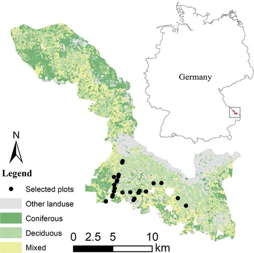
The study area is located in the southern part of the Bavarian Forest National Park, a mixed temperate forest located in the southeast of Germany (49°3ʹ19”N, 13°12ʹ9”E). The park covers an area of 24,250 ha with elevations ranging from 600 to 1453 m. The main vegetation types found in the park include deciduous forest, coniferous forest, mixed forest, meadows, lying deadwood, and standing deadwood. The dominant tree species are Norway spruce (Picea abies) (67%) and European beech (Fagus sylvatica) (24.5%) (Cailleret, Heurich, and Bugmann 2014).

We conducted fieldwork in July 2019. We selected 24 forest plots (Figure 1 and Table 1), each with a radius of 20 m, from the 197 permanent plots established by the Bioklim project (Bässler et al. 2008). Two main criteria were used to select these plots. Firstly, the plots selected were not to have an average slope greater than 10 degrees, as the main goal of this study was to investigate visual obstruction by vegetation, not by terrain. A 5 m resolution digital elevation model (DEM) derived from ALS data was used to determine slope. Secondly, to capture vegetation conditions (i.e., forest type and understory cover), we applied a conditioned Latin Hypercube Sampling (cLHS) method to make a final selection from the remaining plots. cLHS is a stratified random procedure that provides an efficient way of sampling variables from their multivariate distributions (Minasny and McBratney 2006). In this study, we used both forest type and understory cover as input cLHS variables. The understory cover was estimated from ALS data by computing the ratio between the number of understory non-ground points (0.5–2 m high) and all understory points (0–2 m high), which is a popular LiDAR-derived metric that is often used in characterizing understory vegetation density (Campbell et al. 2018).

Table 1. The basic information of the 24 forest plots. The three coverage levels of understory vegetation are low (<18%), medium (18–34%), and high (>34%)

Plot ID	Elevation (m)	Slope (°)	Understory cover (%)	Understory cover level	Forest type
1	935	9.39	2	low	deciduous
2	842	9.13	7	low	deciduous
3	862	8.54	17	low	deciduous
4	843	6.56	21	medium	deciduous
5	930	8.33	23	medium	deciduous
6	932	6.10	34	medium	deciduous
7	1076	7.35	46	high	deciduous
8	766	1.60	47	high	deciduous
9	866	9.63	3	low	coniferous
10	777	0.87	8	low	coniferous
11	853	7.67	11	low	coniferous
12	752	3.13	18	medium	coniferous
13	802	9.02	25	medium	coniferous
14	779	9.98	28	medium	coniferous
15	740	3.68	35	high	coniferous
16	1045	6.38	45	high	coniferous
17	788	5.83	5	low	mixed
18	800	3.58	10	low	mixed
19	764	6.64	19	medium	mixed
20	771	6.59	23	medium	mixed
21	829	8.19	35	high	mixed
22	828	5.21	39	high	mixed
23	803	7.25	42	high	mixed
24	857	8.46	44	high	mixed

Figure 1. The location and distribution of sampling plots in the Bavarian Forest National Park, Germany

The dominant tree species in the coniferous and deciduous forest plots were spruce and beech, respectively; while the mixed plots contained both spruce and beech. In order to investigate the potential impact of the understory cover on the accuracy of the visibility estimation, we binned the understory cover into three levels, i.e., low (<18%), medium (18–34%), and high (>34%), based on understory cover frequency distributions of all sample plots (n = 24). This classification suited the terrain and compared well to informal descriptions of cover by expert national park employees.

2.2. Data collection

2.2.1. TLS data

The TLS used in this study was a time-of-flight scanner RIEGL VZ-400 (Riegl LMS GmbH, Horn, Austria), which employed a pulsed laser operating at λ = 1550 nm, in the shortwave infrared part of the spectrum. The laser beam was 7 mm in diameter as it left the device. The system had a beam divergence of 0.35 mrad, a range accuracy of 5 mm, and an effective measurement rate of 122,000 measurements/second. The pulse energy followed a Gaussian distribution within the laser beam. The data were acquired in long-range mode, with 360° horizontal and 100° (upward 60°/downward 40°) vertical scan angle ranges, and an angular step of 0.04° both horizontally and vertically.

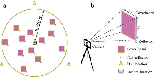
The diagram of a typical sample plot is shown in Figure 2a. In each plot, we chose a center scanning point, surrounded by a triangle of three other scan positions to cover the whole plot (Wilkes et al. 2017). To minimize uncertainty and for better registration of scans, we placed 12 cylindrical reflectors as control points in each plot within the scanner’s field of view and range, in such a way that, from one TLS position, at least three common reflectors can be identified from both it and anyone of other three positions.

Figure 2. (a) A schematic of the sample plot design with a radius of 20 m, (b) the setup with cover board, reflector, and camera

2.2.2. Photography data

We constructed a 1 × 1 m magenta cover board using heavy-duty canvas and a light wooden frame (Figure 2b). The color magenta was adopted because its spectral separability from vegetation is highest, as suggested by Campbell et al. (2018). Besides being used to register the TLS data collection points, the reflectors were also used for the positioning of the cover board by, each time, placing a corner of the cover board next to a reflector (Figure 2b). The result was 12 cover board photos per plot. At distances greater than 15 m the cover board was often obscured, while at very close distance most of the board was visible, allowing little discrimination (Nudds 1977). Accordingly, the horizontal distance between the cover boards and the plot center was limited to 5–20 m and the radius of the plot was set to 20 m. For more representativeness, we distributed four cover boards each within the distance intervals 5–10 m, 10–15 m, and 15–20 m. We took photos of the cover board positioned at every reflector position in turn, using a Canon EOS 5D camera mounted on top of a tripod at the plot center. The cover board would be set up facing the plot center and vertically, with the aid of a compass and bubble/spirit level. The relative positions and orientations of cover boards in the co-registered point cloud allowed the simulation of virtual cover board images.

2.3. Estimating visibility from photography

In total, we obtained 288 cover board photos (24 plots × 12 photos) in the field. We performed an automated board versus non-board (i.e., pixels inclusively containing anything besides the cover board, primarily live and dead vegetation) classification procedure, modified from the one described by Campbell et al. (2018). Firstly, we cropped the extent of the cover board in every photo using ImageJ, a public domain Java image processing program (Schindelin et al. 2015), insuring that at least one pair of diagonal corners of the cover board could be recognized from the photo. There were 257 eligible photos out of all 288 photos. Subsequently, we generated four random points on every cropped photo using a program written in R language (R Core Team 2013), and then visually interpreted each point as either a board or a non-board. As a result, there were 1028 (257 photos × 4 points) sampling points in total, comprising 360 non-board points and 468 board points. From all sampling points, we randomly designated 200 points as test data (100 board points, 100 non-board points) and used the remainder as training data.

For each point, we extracted the mean pixel values from the red, green, and blue (RGB) channels within a 5 × 5 window size. To improve the classification accuracy, we also calculated a number of derivative variables from RGB values (Table 2). We performed a stepwise logistic regression using the “caret” package (Kuhn 2008) in R version 3.5.1 (R Core Team 2013). The regression began with a full model that contained all of the independent variables in Table 2 and iteratively removed them until an optimal balance between model complexity and variance remained, as approximated by the Akaike Information Criterion (AIC). Using the derived regression model, we classified every pixel of every photo as a board (1), when the predicted value was greater than or equal to 0.5, or as a non-board (0), when the predicted value was less than 0.5. Lastly, we calculated the photography-derived visibility as the proportion of the non-board pixels in each binary classification photo. We assessed the overall and class-specific user’s and producer’s accuracies of the photo classification using the independent test data.

Table 2. The spectral variables used in the stepwise logistic regression to classify board versus non-board on the cover board photos

Variable	Abbreviation	Calculation
Red	R	8-bit R pixel mean
Green	G	8-bit G pixel mean
Blue	B	8-bit B pixel mean
Normalized red	$R_{norm}$	R/(R + G + B)
Normalized green	$G_{norm}$	G/(R + G + B)
Normalized blue	$B_{norm}$	B/(R + G + B)
Magenta	M	(R + B)/2
Cyan	C	(B + G)/2
Yellow	Y	(G + R)/2
Normalized magenta	$M_{norm}$	M/(M + C + Y)
Normalized cyan	$C_{norm}$	C/(M + C + Y)
Normalized yellow	$Y_{norm}$	Y/(M + C + Y)
Normalized difference red-green	NDRG	(R – G)/(R + G)
Normalized difference green-blue	NDGB	(G – B)/(G + B)
Normalized difference blue-red	NDBR	(B – R)/(B + R)
Normalized difference magenta-cyan	NDMC	(M – C)/(M + C)
Normalized difference cyan-yellow	NDYC	(C – Y)/(C + Y)
Normalized difference yellow-magenta	NDYM	(Y – M)/(Y + M)

2.4. Estimating visibility from TLS

2.4.1. TLS data preprocessing

Because the return signal from a TLS contains ghost point errors (i.e., a mixture of return signal forms of multiple objects), the signal shape always deviates from a Gaussian distribution (Béland et al. 2014). This pulse shape deviation may be interpreted as a measure of the reliability of the range measurements (Pfennigbauer and Ullrich 2010). The overall quality of the point cloud can be improved by setting a maximum allowed deviation value. In this study, all ghost points with a deviation above 20 were removed using RiScan software (http://www.riegl.com). This deviation threshold was adopted based on suggestions from previous studies (Pfennigbauer and Ullrich 2010; Greaves et al. 2015).

In this study, the goal of registering point cloud datasets recorded from different locations was not only to minimize the occlusion effect and improve the quality of the data, but also to obtain the position of every reflector in the global coordinate system, as this formed the foundation for simulating virtual cover board images. We used RiScan software to register the point cloud dataset, where the central scan position was designated as a reference scan and matched to the three other scanning points, placed around it in a triangular fashion. As a result, the starting point in the global coordinate system was at the central TLS position. Given that horizontal distance from the cover boards to the plot center was limited to 20 m, we clipped all points from the co-registered point cloud where the horizontal distance to the origin was greater than 20 m.

2.4.2. Occupancy grid establishment

An occupancy grid is a location-based representation of the environment. It divides the space into a regular grid of 2D or 3D cells and estimates the probability of any cell being “occupied” by objects, based on the sensor measurements (Moravec and Elfes 1985; Elfes 1989). Establishing a 3D occupancy grid based on the TLS point cloud is the process of voxelizing the point cloud.

Let s denote the proposed 3D occupancy grid map. A single grid voxel is denoted as $s_{x,y,z}$, while $m_1,\dots ,m_n$ denote all of the TLS points collected at each scanning position. Each voxel corresponds to a binary value, which specifies whether it is occupied or not. The notation P($s_{x,y,z}=1$) is used to denote an occupied voxel. The problem addressed by occupancy grid mapping is determining the posterior:

(1) $\mathrm{P}(s|m_1,\dots ,m_n)$(1)

given all TLS points. However, as the grid maps are defined in 3D, this posterior cannot be easily computed. The classical occupancy grid algorithm breaks down the problem into many 1D estimation problems, treating each voxel independently. The problem is thus reduced to the estimation of the posterior for each $s_{x,y,z}$ of the grid:

(2) $\mathrm{P}(s_{x,y,z}|m_1,\dots ,m_n)$(2)

For computational reasons, it is common to calculate the so-called log-odds of $\mathrm{P}(s_{x,y,z}|m_1,\dots ,m_n)$ instead of estimating the posterior $\mathrm{P}(s_{x,y,z}|m_1,\dots ,m_n)$. The log-odds are defined as follows:

(3) $l_{x,y,z}^n=\mathrm{l}\mathrm{o}\mathrm{g}\frac{\mathrm{P}(s_{x,y,z}|m_1,\dots ,m_n)}{1-\mathrm{P}(s_{x,y,z}|m_1,\dots ,m_n)}$(3)

From the log-odds $l_{x,y,z}^n$ defined in (3), the posterior occupancy probability can then be “recovered.” Under the static world assumption, the log-odds conditioned on n points are estimated recursively via Bayes’s rule, and applied to the posterior $\mathrm{P}(s_{x,y,z}|m_1,\dots ,m_n)$

(4) $log\frac{P\left(s_{x,y,z}|m_1,\dots ,m_n\right)}{1-P\left(s_{x,y,z}|m_1,\dots ,m_n\right)}=log\frac{P\left(s_{x,y,z}|m_n\right)}{1-P\left(s_{x,y,z}|m_n\right)}+log\frac{1-P\left(s_{x,y,z}\right)}{P\left(s_{x,y,z}\right)}+log\frac{P(s_{x,y,z}|m_1,\dots ,m_{n-1})}{1-P(s_{x,y,z}|m_1,\dots ,m_{n-1})}$(4)

Inserting the log-odds $l_{x,y,z}^n$ as defined in equation (3)(3) $l_{x,y,z}^n=\mathrm{l}\mathrm{o}\mathrm{g}\frac{\mathrm{P}(s_{x,y,z}|m_1,\dots ,m_n)}{1-\mathrm{P}(s_{x,y,z}|m_1,\dots ,m_n)}$(3) , we arrive at the recursive equation:

(5) $l_{x,y,z}^n=\mathrm{l}\mathrm{o}\mathrm{g}\frac{\mathrm{P}(s_{x,y,z}|m_{\mathrm{n}})}{1-\mathrm{P}(s_{x,y,z}|m_n)}+\mathrm{l}\mathrm{o}\mathrm{g}\frac{1-\mathrm{P}\left(s_{x,y,z}\right)}{\mathrm{P}\left(s_{x,y,z}\right)}+l_{x,y,z}^{n-1}$(5)

with the initialization

(6) $l_{x,y,z}^0=\mathrm{l}\mathrm{o}\mathrm{g}\frac{\mathrm{P}\left(s_{x,y,z}\right)}{1-\mathrm{P}\left(s_{x,y,z}\right)}$(6)

Assuming that a prior probability for each voxel being occupied is $\mathrm{P}\left(s_{x,y,z}\right)$=0.5, the estimation problem simply becomes to update the log-odds $l_{x,y,z}^n$ of each voxel given the $\mathrm{P}(s_{x,y,z}|m_{\mathrm{n}})$.

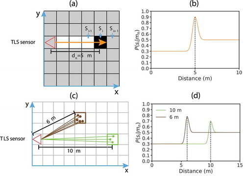
$\mathrm{P}{(}_{x,y,z}|m_{\mathrm{n}})$ is an inverse sensor model since it maps TLS points back to their starting parameters. In this study, we adopted an inverse sensor model that combines a linear and Gaussian function, with an importance factor k and distance measurement uncertainty σ (Pirker et al. 2011). If $s_i$ denotes the i-th voxel, which lies on the traveling path of the laser beam that raised the TLS point $m_n$ (Figure 3a), the probability that $s_i$ is occupied conditioned on the TLS point $m_n$ forms the continuous function:

(7) $P(s_i\left|m_n\right.)\left\{\begin{array}{c}0.3+\left(\frac{k}{\sigma \sqrt{2\pi }}+0.2\right)e^{-\frac{1}{2}{\left(\frac{d_{n,i^{-d_n}}}{\sigma }\right)}^2}\\ 0.5+\left(\frac{k}{\sigma \sqrt{2\pi }}\right)e^{-\frac{1}{2}\left(\frac{d_{n,i^{-d_n}}}{\sigma }\right)}if{d}_n\ge d_{n,i}\end{array}if0\le d_n\le d_{n,i}\right.$(7)

Figure 3. Illustration of occupancy grid mapping: (a) A 2D example of mapping the occupancy probabilities of the cells affected by one laser beam. The orange arrow represents a laser beam. $d_n$ is the distance from the point $m_n$ to the TLS sensor origin. $s_i$ is the i-th voxel which lies on the traveling path of the laser beam that raised the point $m_n$. Lower probabilities are encoded in white, higher probabilities in black. The unmapped cells are gray. (b) Inverse sensor model for one laser beam. Occupancy probability values for the distance measure at 5 m. (c) A 2D example of mapping the occupancy probabilities of two cells affected by several laser beams. One cell at 6 m from the TLS sensor contains five points, and another one at 10 m from the TLS sensor contains three points. The brown and green solid lines and dots represent laser beams and points, respectively. (d) The resulting occupancy probability values for the two cells in (c)

where $d_n$ is the distance from the point $m_n$ to the TLS sensor origin; $d_{n,i}$ is the distance from the voxel $s_i$ to the TLS sensor origin; while parameter $k=\sigma =0.6$. The main idea of this approach is that the probability of a voxel being occupied (i) near a point (in the point cloud) is high (the laser beam likely hits this voxel), (ii) between the sensor and a point is low (the laser beam passes through this voxel), and (iii) beyond a point is unchanged (the space behind the occupied voxel is not scanned by the laser beam) (Figure 3b). The occupancy probability value of a single voxel will be updated according to the contribution of all laser beams using equations (5)(5) $l_{x,y,z}^n=\mathrm{l}\mathrm{o}\mathrm{g}\frac{\mathrm{P}(s_{x,y,z}|m_{\mathrm{n}})}{1-\mathrm{P}(s_{x,y,z}|m_n)}+\mathrm{l}\mathrm{o}\mathrm{g}\frac{1-\mathrm{P}\left(s_{x,y,z}\right)}{\mathrm{P}\left(s_{x,y,z}\right)}+l_{x,y,z}^{n-1}$(5) – (7(7) $P(s_i\left|m_n\right.)\left\{\begin{array}{c}0.3+\left(\frac{k}{\sigma \sqrt{2\pi }}+0.2\right)e^{-\frac{1}{2}{\left(\frac{d_{n,i^{-d_n}}}{\sigma }\right)}^2}\\ 0.5+\left(\frac{k}{\sigma \sqrt{2\pi }}\right)e^{-\frac{1}{2}\left(\frac{d_{n,i^{-d_n}}}{\sigma }\right)}if{d}_n\ge d_{n,i}\end{array}if0\le d_n\le d_{n,i}\right.$(7) ). The more laser beams that “hit” a voxel, the higher probability that it is occupied, whereas the more laser beams that “traverse” a voxel, the higher probability that it is free. A simplified, 2D example of mapping the occupancy probabilities of the cells affected by several laser beams is shown in Figure 3c. The resulting occupancy probability value of the brown cell is higher than of the green one because more laser beams hit the brown cell (Figure 3d). After updating, each voxel will be labeled either “occupied” or “free,” or “unmapped” if not hit or traversed by any pulse.

To complete the update, we used a ray-tracing algorithm to determine the cells that are affected by the pulse raising a point. Because a single pulse beam of TLS is cone-shaped, it can overlap with multiple voxels far from the origin, which causes the undesired Moiré effect (Yguel, Aycard, and Laugier 2008). The diameter of the beam can be calculated using the following equation (Petrie and Toth 2008):

(8) $D=Di\times BDv+BDm$(8)

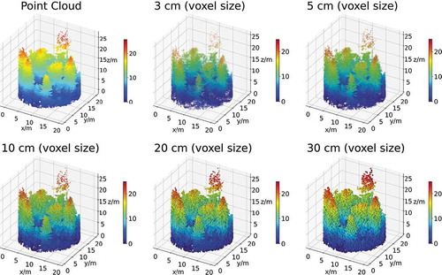
where D is the diameter of the laser footprint; Di is the traveling distance of the laser beam; BDv is the beam divergence in radians; BDm is the beam diameter at exit of the scanner (Supplementary Figure 1). According to relevant TLS parameters in this study, the pulse diameter was 1.4 cm at 20 m, which constituted the maximum horizontal distance from a cover board to a TLS position. To reduce multiple overlaps between the laser beam and voxels, we used and tested five different voxel sizes larger than 1.4 cm to build the occupancy grid, i.e., 3 cm, 5 cm, 10 cm, 20 cm, 30 cm. We assumed the diameter of the pulse beam was infinitesimally small, to simplify the ray-tracing procedure. Further, we assumed that occupied voxels in the line of sight were completely opaque, while free and unmapped voxels were completely transparent.

Procedures given above for establishing a 3D occupancy grid map were algorithmized using log-odds representation (Table 3). We implemented this algorithm based on OctoMap, which is an open-source framework to generate volumetric 3D environment models. The mapping approach in OctoMap is based on octrees and uses probabilistic occupancy estimation (Hornung et al. 2013). Figure 4 shows voxelization of an example plot through occupancy grid mapping for each investigated voxel size.

Table 3. The standard occupancy grid mapping algorithm, shown here using log-odds representations

/* Initialization */ for all grid voxels (x, y, z) dolx,y,z = log p(sx,y,z) –log[1–p (sx,y,z)]endfor /* Grid update using log-odds */ for all points t from 1 to n do for all grid cells (x, y, z) in the perceptual range of do lx,y,z = lx,y,z +log p(sx,y,z Vmt) –log[1–p(sx,y,z) Vmt] +log[1–p(sx,y,z)] endfor endfor /* Recovery of occupancy probabilities */ for all grid cells (x, y, z) doendfor

Figure 4. Illustration of the voxelization of a sample point cloud (Plot 12) using five different voxel sizes

2.4.3. Simulating virtual cover board images

To calculate visibility from TLS, we simulated 257 virtual cover board images using a ray-tracing method based on the occupancy grid model. Location, orientation as well as size of each virtual cover board image were kept equal to those of the corresponding real cover board photo. Firstly, we computed the position and orientation of each cover board in a global coordinate system from the position of the corresponding reflector and the azimuth measured by a compass, respectively. We also calculated the coordinates of the camera center by subtracting the height difference between the TLS and camera center from the origin of the coordinate system at the TLS center. The pixel size of the virtual cover board image was determined at 1 cm, i.e., approximately equal to the smallest pulse diameter of 0.88 cm at 5 m, which was the closest distance of the cover boards to the plot center. The TLS pulse cannot differentiate an object smaller than the pulse diameter. To determine the visibility of every pixel, we traced the line of sight from the camera center to every pixel center of the virtual image through the established occupancy grid using the voxel traversal algorithm (Amanatides and Woo 1987). If the line of sight was obstructed by any occupied voxel in between, the corresponding pixel value was 1, representing a non-board. If the line of sight was not obstructed, the corresponding pixel value was 0, representing a board. Lastly, we calculated the TLS-derived visibility as the proportion of non-board pixels in each virtual binary cover board image.

2.5. Comparison of TLS-based and photography-based visibility estimates

We quantitatively compared estimates of visibility at individual photo level (n = 257) derived from TLS to those derived from photography. To determine the effects of voxel size, forest type, understory cover, and their interactions on the accuracy of visibility estimation, we conducted a 5 (voxel size) × 3 (forest type) × 3 (understory cover) factorial ANOVA analysis in R version 3.5.1 (R Core Team 2013). We split our data into different subsets, each of which comprised a different set of voxel size, forest type, and understory cover conditions. For every combination of these three factors, there were on average 29 samples (ranging from 24 to 32). We further partitioned these samples into four subsets evenly. For each data subset, we regressed photography-derived visibility (observed values) on TLS-derived visibility (predicted values), from which coefficient of determination ($R^2$) and root-mean-square error (RMSE) were calculated. As a result, there were four observations under every combination of the factors for the three-way ANOVA. In this manner, we calculated F-value and probability (p-value) indicating significance levels, as well as partial eta squared (partial ${\eta }^2$) indicating to what extent explanatory factors have a relative effect. Tukey’s HSD pairwise comparisons test was used to compare individual means. The level of significant difference was assessed at p < 0.05. Before analyzing the results, data were checked for normality and equality of variances using the Shapiro–Wilk and Hartley–Bartlett tests, respectively. In all cases, key assumptions of ANOVA were met.

3. Results

3.1. Accuracy of visibility estimated from photography

In total, 257 cover board photos were classified into a binary image representing board and non-board areas from which visibility values were calculated (Figure 5). Randomly selected test points were compared to the classification results. The photography-based approach achieved an overall accuracy of 95% (Table 4).

Table 4. The confusion matrix for the classification results of cover board photos

		Reference		Accuracy
		Board	Non-board	User	Producer	Overall
Prediction	Board	94	4	96%	94%	95%
	Non-board	6	96	94%	96%

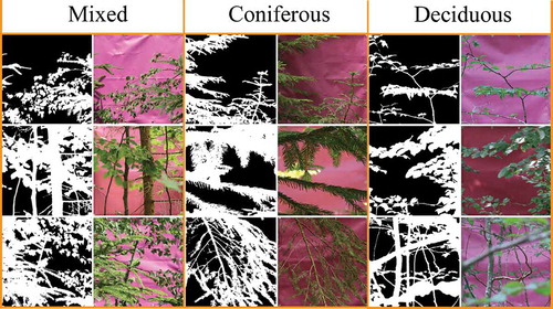
Figure 5. An example of the classification results of the cover board photos. The left, middle, and right panels correspond to the mixed, coniferous, and deciduous forest plots, respectively. In binary images, black areas indicate pixels classified as a board and white areas indicate pixels classified as a non-board

3.2. Comparison between visibility estimated from TLS and photography

The effects of forest type, understory cover, voxel size, and their interaction on forest visibility, as derived by photography and TLS, are detailed in Table 5. The interaction between understory cover and forest type had a significant effect on both $R^2$ and RMSE; while the interaction between understory cover and voxel size only had a significant effect on $R^2,$ but not on RMSE. Furthermore, the interaction between forest type, understory cover, and voxel size had no significant effect on the agreement between photography-derived and TLS-derived visibility. However, voxel size, forest type, and understory cover independently had a significant effect on both $R^2$ and RMSE.

Table 5. Summary of results from a factorial ANOVA showing the effects of forest type, understory cover, voxel size, and their interaction on the agreement between photography-derived and TLS-derived visibility

Response variables	Factors	SS	d.f.	MS	F-value	p-value	Partial ${\eta }^2$
$R^2$	Forest type	0.427	2	0.2137	46.65	0.000*	0.41
	Understory cover	0.362	2	0.1812	39.53	0.000*	0.37
	Voxel size	6.950	4	1.7375	379.22	0.000*	0.92
	Forest type × Understory cover	0.297	4	0.0742	16.20	0.000*	0.32
	Forest type × Voxel size	0.035	8	0.0044	0.96	0.469	0.05
	Understory cover × Voxel size	0.076	8	0.0095	2.08	0.042*	0.11
	Forest type × Understory cover × Voxel size	0.102	16	0.0063	1.39	0.158	0.14
	Residuals	0.619	135	0.0046	-	-	-
RMSE	Forest type	274.7	2	137.3	16.19	0.000*	0.19
	Understory cover	589.9	2	295.0	34.77	0.000*	0.34
	Voxel size	2872.9	4	718.2	84.67	0.000*	0.72
	Forest type × Understory cover	322.1	4	80.5	9.50	0.000*	0.22
	Forest type × Voxel size	99.7	8	12.5	1.47	0.174	0.08
	Understory cover × Voxel size	59.3	8	7.4	0.86	0.540	0.05
	Forest type × Understory cover × Voxel size	161.1	16	10.1	1.19	0.286	0.12
	Residuals	1145.2	135	8.5	-	-

SS = sum of squares, d.f. = degrees of freedom, MS = mean square, * p < 0.05.

As depicted in Figure 6a, the highest accuracy was obtained with a 10 cm voxel. The mean $R^2$ significantly increased from 0.30 to 0.76 when the voxel size decreased from 30 cm to 10 cm. Further decreasing the voxel size from 10 cm to 3 cm resulted in a decrease in $R^2$ from 0.76 to 0.71. The mean RMSE showed an inverse trend, significantly declining from 24.63% to 14.61% at 10 cm, before increasing slightly to 15.78% at smaller voxel size. The detailed results regarding voxel size are shown in Supplementary Figure 2.

Figure 6. The mean of $R^2$ and RMSE between photography-derived and TLS-derived visibility (a) for five different voxel sizes: 3 cm, 5 cm, 10 cm, 20 cm, 30 cm, (b) for three forest types: deciduous, coniferous, and mixed, and (c) three levels of understory cover: low, medium, and high. The different letters inside the figures indicate a statistically significant difference between different combinations of these three factors. The same letter indicates no significant difference (Tukey’s HSD test, p < 0.05)

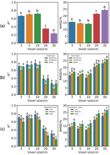
The mean $R^2$ and RMSE suggested that the lowest errors for TLS-derived visibility estimates were achieved with a voxel size of 10 cm regardless of forest type; while the trends of $R^2$ as well as RMSE with an increasing voxel size were similar for deciduous, coniferous, and mixed forest plots (Figure 6b). The RMSE values for the mixed and coniferous plots were often significantly higher than for the deciduous plots. The $R^2$ values for the coniferous plots were significantly lower than for the deciduous and mixed plots. The overall estimation accuracy for the deciduous forest plots was higher than for the coniferous and mixed plots. The detailed results regarding forest type are shown in Supplementary Figure 3.

In general, a significant inhibitory effect on estimation accuracy was evident with a higher cover of understory. Increased understory cover significantly decreased the mean $R^2$ and increased the mean RMSE (Figure 6c). In addition, the mean $R^2$ of TLS-derived visibility was significantly higher with a 5 cm voxel than with a 10 cm voxel for forest plots with a high understory cover (p = 0.038), while there was no significant difference in the mean RMSE. Therefore, 5 cm was seen as the optimal voxel size for forest plots with high understory cover, while the highest accuracy for forest plots with either low or medium understory cover was obtained using a 10 cm voxel. The detailed results regarding the understory cover are shown in Supplementary Figure 4.

Considering both $R^2$ and RMSE, the effect of voxel size is predominant on visibility estimation, followed by understory cover and forest type (Table 5). Overall, TLS-derived visibility had highest agreement with photography-derived visibility under different forest types and understory cover conditions with a 10 cm voxel (Table 6).

Table 6. The agreement ($R^2$ and RMSE) between photography-derived and TLS-derived visibility under different forest types and understory cover conditions using a voxel size of 10 cm

	Forest type			Understory cover			overall
	Deciduous	Coniferous	Mixed	Low	Medium	High
$R^2$	0.79	0.73	0.73	0.77	0.72	0.67	0.77
RMSE (%)	12.45	14.34	16.07	13.37	13.74	17.29	14.33

3.3. Sensitivity analysis of voxel size and understory cover on unmapped voxels

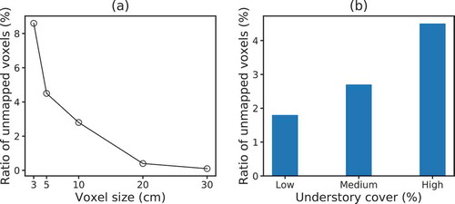
The influence of voxel size and understory cover on the amount of the unmapped voxels in relation to the total volume is shown in Figure 7. The average ratio of unmapped voxels of all the 24 plots decreased more or less exponentially from 8.6% to 0% when the voxel size was increased from 3 cm to 30 cm. A sharp decrease occurred at smaller voxel sizes from 3 cm to 10 cm; and a very small decrease occurred at larger voxel sizes between 20 cm and 30 cm (Figure 7a). The average ratio of unmapped voxels increased from 1.8% to 4.5% with increasing understory cover for a voxel size of 10 cm (Figure 7b).

Figure 7. (a) The relationship between the average ratio of unmapped voxels of all 24 plots and voxel size, (b) the average ratio of unmapped voxels of all 24 plots for different levels of understory cover given a voxel size of 10 cm

4. Discussion

In this study, we presented a TLS-based approach to estimate fine-scale visibility in a mixed temperate Central European forest and compared the results with those derived from the gold-standard photography-based approach. Moreover, we examined the potential impact of voxel size, forest type, and understory cover on estimation accuracy.

The selection of a suitable voxel size played an essential role in estimating visibility using TLS. The optimal voxel size represents a compromise among factors including point spacing, pulse diameter, and occlusion rate of voxels (Cifuentes et al. 2014; Kükenbrink et al. 2017; Béland et al. 2014). When estimating visibility using TLS-based approaches, the optimal voxel size needs to be small enough to account for detailed vegetation structure, including geometric shapes of vegetation elements and internal gaps, but large enough for the ratio of unmapped voxels to remain low, in order to increase the robustness of the occupancy inference. The optimal voxel size of 10 cm found in this study supports the hypothesis of Béland et al. (2014) that optimal voxel sizes for characterization of forest canopy using TLS may range from 5 to 20 cm. We confirm the results of Kükenbrink et al. (2017) who found that a smaller voxel size significantly increased the number of unmapped voxels, encompassing occluded and unobserved voxels. Because the unmapped voxels were neither hit nor traversed by any pulse, there was no information to infer their occupancy state, causing a high ratio of unmapped voxels to have a low estimated visibility accuracy. As depicted in Figure 7a, a smaller voxel size had a higher high ratio of unmapped voxels, and in turn caused a lower accuracy. Tree movement due to wind is also a source of uncertainty, as laser returns from the same target can be located in different voxels for different laser acquisitions. Applying a voxel size larger than the pulse diameter (approx. 7 times larger for the 10 cm voxel size) can reduce this effect (Kükenbrink et al. 2017). However, unlike wind, which may displace laser returns, fog, dew, and rain can decrease the detection distance as well as the number of points, making it difficult to mitigate by adjusting voxel size (Wojtanowski et al. 2014; Goodin et al. 2019; Kutila et al. 2018). Therefore, good weather conditions are required for the application of TLS when assessing visibility.

The results suggest that understory cover influenced not only the selection of an optimal voxel size but also the level of accuracy that can be achieved given the optimal voxel size. Whereas the optimal voxel size for forest plots with low or medium understory cover was 10 cm, the optimal voxel size decreased to 5 cm for forest plots with high understory cover. The significant interaction between understory cover and voxel size implies the effect of voxel size can vary with different levels of understory cover, which coincides with the changing of optimal voxel size. A forest plot with high understory cover has a complex vegetation structure resulting in smaller and more complex gaps than plots with sparse understory have. Therefore, a smaller voxel size is required for denser understory cover to account for the detailed vegetation structure, although the ratio of the unmapped voxels may increase. Since the highest percentage of understory cover in this study was 47% (Table 1), more research is required to investigate whether the optimal voxel size needs to be decreased further if the understory is even denser than 47%. Denser understory caused more occlusion in the TLS data, which in turn increased the ratio of unmapped voxels (Figure 7b). As a result, the accuracy in estimating visibility decreased with increasing understory cover. In addition, occlusion will also increase along the traveling distance of the laser beam. In TLS, the spherical scanning geometry leads to a higher point density within close range of the sensor, than far away from it (Jupp et al. 2009; Zhao et al. 2015). The point cloud density decreases with distance in forests due to the occlusion effect, which in turn may affect visibility estimation. Scanning at multiple locations has shown to reduce occlusion and substantially improve the quality of datasets (Van der Zande et al. 2006; Wilkes et al. 2017). To examine the potential effect of the traveling distance of the laser beam on visibility estimation while using multiple scanning strategies, we conducted a one-way ANOVA analysis as introduced previously. All samples were split into four subsets according to the distance between the cover boards and the central scanning position of the TLS sensor, with every subset having a respective distance level of either 5, 10, 15, or 20 m. The results are shown in Table 7. We found that the traveling distance of the laser beam had no significant effect on either $R^2$ or RMSE for a plot with a 20 m radius. Our findings suggest that multi-scan settings as used in this study can effectively reduce occlusion effects caused by the traveling distance of the laser beam. Therefore, multiple TLS scanning is highly recommended for dense forest plots in order to reduce the potential occlusion effect in such studies.

Table 7. Summary of results from a one-way ANOVA showing the effect of the traveling distance of the laser beam on the agreement between photography-derived and TLS-derived visibility

Response variables	Factors	SS	d.f.	MS	F-value	p-value
$R^2$	Distance	0.010	3	0.0034	0.549	0.654
	Residuals	0.125	20	0.0063	-	-
RMSE	Distance	18.05	3	6.017	1.191	0.338
	Residuals	101.02	20	5.051	-

SS = sum of squares, d.f. = degrees of freedom, MS = mean square, p < 0.05.

As the results demonstrate, the optimal voxel sizes were the same for deciduous, coniferous, and mixed forest plots. What can be inferred is that forest type had little impact on the determination of the optimal voxel size. We found that our approach performed better for deciduous forest plots than for coniferous and mixed forest plots. The lower accuracy achieved for coniferous and mixed plots may have been due to the gaps between needles within shoot clumps being too small to be accurately differentiated by laser beams. Both the vertical and the horizontal angular steps of TLS used in this study were 0.04${ }^{\circ }$, while the distance between two adjacent laser beams at a range of 20 m was 1.4 cm. As a result, all gaps between leaves larger than 1.4 cm could be differentiated by laser beams in our study. However, if the number of very tiny gaps increases, the ability of TLS to differentiate these gaps may be reduced, thereby possibly decreasing the accuracy of the visibility estimation.

The reasonability of assuming the laser pulse diameter to be infinitesimally small depends on the relative size of the laser pulse diameter compared to the voxel size. The diameter of a laser beam diverges with traveling distance, and consequently, it is cone-shaped. As a result, the number of beams that contribute to the probability of a single voxel is quite large in regions close to the sensor origin. In contrast, a single beam can overlap with multiple voxels far from the origin, which may decrease occupancy prediction accuracy (Homm et al. 2010). What can be inferred is that, for a smaller voxel size, the probability that a beam overlaps with multiple voxels is higher, introducing more uncertainty. Therefore, an infinitesimally small laser pulse diameter is a reasonable assumption when the voxel size is much larger than the pulse diameter. Though this effect is minimal in a 20 m plot, a laser beam may require to be treated as a cone if it is tracked much further away.

5. Conclusion

Our study showed that there was good agreement between the visibility derived from TLS-based and photography-based approaches. Voxel size had a strong effect on visibility estimates; and the most accurate estimates were obtained at a voxel size of 10 cm. In general, the TLS-based approach performed better in deciduous forest plots than in coniferous and mixed forest plots, though forest type had little effect on the optimal voxel size. The understory had a significant effect on the estimates, with lower accuracy in dense understory cover. The optimal voxel size decreased from 10 cm for low and medium understory cover to 5 cm for high understory cover. Our findings highlight the use of the TLS technique as a method for rapidly estimating fine-scale visibility in forests. More importantly, TLS provides the opportunity to move beyond estimating visibility at single locations and from limited perspectives, to its estimation at any location and from any perspective within a scanned area, thereby greatly improving sampling efficiency. We believe that the proposed TLS-based approach has great potential for the study of animal behavior (e.g., predator–prey relationships) in forest landscapes.

Data and Codes Availability Statement

The data and codes that support the findings of this study are available on request from the corresponding author, (X.Z). The data are not publicly available because they contain information that could compromise the privacy of research participants.

Acknowledgements

The authors acknowledge the support of the Chinese Government Scholarship under the grant number [201704910852] and the European Commission’s Horizon 2020 research and innovation program—‘BIOSPACE Monitoring Biodiversity from Space’ project under the grant agreement number [834709], and the “Data Pool Forestry” data sharing initiative of the Bavarian Forest National Park. We would also like to thank Dr. Fiderer Christian from the Bavarian Forest National Park for his support with the field work.

Disclosure statement

No potential conflict of interest was reported by the authors.

Additional information

Funding

This work was supported by the Chinese Government Scholarship under the grant number [201704910852] and the European Commission’s Horizon 2020 research and innovation program under the grant agreement number [834709].

References

- Amanatides, J., and A. Woo. 1987. “A Fast Voxel Traversal Algorithm for Ray Tracing.” In Eurographics, 87:3–10. Amsterdam: Blackwell.
- Bässler, C., B. Förster, C. Moning, and M. Jörg 2008. “The BIOKLIM-Project: Biodiversity research between climate change and wilding in a temperate montane forest–the conceptual framework.” Waldökologie, Landschaftsforschung und Naturschutz 7:21–33.
- Batty, M. 2001. “Exploring isovist fields: Space and shape in architectural and urban morphology.” Environment and Planning. B, Planning & Design 28 (1):123–150. doi: 10.1068/b2725
- Béland, M., D. D. Baldocchi, J.-L. Widlowski, R. A. Fournier, and M. M. Verstraete. 2014. “On seeing the wood from the leaves and the role of voxel size in determining leaf area distribution of forests with terrestrial lidar.” Agricultural and Forest Meteorology 184:82–97. doi: 10.1016/j.agrformet.2013.09.005
- Benedikt, M. L. 1979. “To take hold of space: Isovists and isovist fields.” Environment and Planning. B, Planning & Design 6 (1):47–65. doi: 10.1068/b060047
- Bienert, A., R. Queck, A. Schmidt, C. Bernhofer, and H. G. Maas. 2010. “Voxel space analysis of terrestrial laser scans in forests for wind field modelling.” International Archives of Photogrammetry, Remote Sensing and Spatial Information Sciences 38 (Part 5):92–97.
- Boyd, C. S., and T. J. Svejcar. 2005. “A visual obstruction technique for photo monitoring of willow clumps.” Rangeland Ecology & Management 58 (4):434–438. doi: 10.2111/1551-5028(2005)058[0434:AVOTFP]2.0.CO;2
- Cailleret, M., M. Heurich, and H. Bugmann. 2014. “Reduction in browsing intensity may not compensate climate change effects on tree species composition in the bavarian forest national park.” Forest Ecology and Management 328:179–192. doi: 10.1016/j.foreco.2014.05.030
- Caldwell, D. R., J. Ehlen, and R. S. Harmon. 2005. Studies in Military Geography and Geology. Dordrecht: Kluwer Academic Publishers.
- Campbell, M. J., P. E. Dennison, A. T. Hudak, L. M. Parham, and B. W. Butler. 2018. “Quantifying understory vegetation density using small-footprint airborne lidar.” Remote Sensing of Environment 215:330–342. doi: 10.1016/j.rse.2018.06.023.
- Carlyle, C. N., L. H. Fraser, C. M. Haddow, B. A. Bings, and W. Harrower. 2010. “The use of digital photos to assess visual cover for wildlife in rangelands.” Journal of Environmental Management 91 (6):1366–1370. doi: 10.1016/j.jenvman.2010.02.018
- Cifuentes, R., D. Van der Zande, J. Farifteh, C. Salas, and P. Coppin. 2014. “Effects of voxel size and sampling setup on the estimation of forest canopy gap fraction from terrestrial laser scanning data.” Agricultural and Forest Meteorology 194:230–240. doi: 10.1016/j.agrformet.2014.04.013
- Dean, D. J. 1997. “Improving the accuracy of forest viewsheds using triangulated networks and the visual permeability method.” Canadian Journal of Forest Research 27 (7):969–977. doi: 10.1139/x97-062
- Eitel, J. U. H., L. A. Vierling, and T. S. Magney. 2013. “A lightweight, low cost autonomously operating terrestrial laser scanner for quantifying and monitoring ecosystem structural dynamics.” Agricultural and Forest Meteorology 180:86–96. doi: 10.1016/j.agrformet.2013.05.012
- Elfes, A. 1989. “Using Occupancy Grids for Mobile Robot Perception and Navigation.” Computer 22 (6):46–57. doi: 10.1109/2.30720
- Goodin, C., D. Carruth, M. Doude, and C. Hudson. 2019. “Predicting the Influence of Rain on LIDAR in ADAS.” Electronics 8 (1):89. doi: 10.3390/electronics8010089
- Greaves, H. E., L. A. Vierling, J. U. H. Eitel, N. T. Boelman, T. S. Magney, C. M. Prager, and K. L. Griffin. 2015. “Estimating aboveground biomass and leaf area of low-stature arctic shrubs with terrestrial LiDAR.” Remote Sensing of Environment 164:26–35. doi: 10.1016/j.rse.2015.02.023
- Griffith, B., and B. A. Youtie. 1988. “Two devices for estimating foliage density and deer hiding cover.” Wildlife Society Bulletin (1973-2006) 16 (2):206–210.
- Hagstrom, S., M. D. Turner, D. Messinger, and G. W. Kamerman. 2011. “Line-of-Sight Analysis Using Voxelized Discrete LiDAR.” In Laser Radar Technology and Applications XVI, 80370B. Orlando, FL: SPIE.
- Higgins, K. F., J. L. Oldemeyer, K. J. Jenkins, G. K. Clambey, and R. F. Harlow. 1996. “Vegetation sampling and measurement.” Research and Management Techniques for Wildlife and Habitats 5:567–591.
- Homm, F., N. Kaempchen, J. Ota, and D. Burschka. 2010. “Efficient Occupancy Grid Computation on the GPU with LiDAR and Radar for Road Boundary Detection.” In 2010 IEEE Intelligent Vehicles Symposium, 1006–1013. San Diego, CA: IEEE.
- Hornung, A., K. M. Wurm, M. Bennewitz, C. Stachniss, and W. Burgard. 2013. “Octomap: An efficient probabilistic 3D mapping framework based on octrees.” Autonomous Robots 34 (3):189–206. doi: 10.1007/s10514-012-9321-0
- Hosoi, F., and K. Omasa. 2006. “Voxel-based 3-D modeling of individual trees for estimating leaf area density using high-resolution portable scanning LiDAR.” IEEE Transactions on Geoscience and Remote Sensing 44 (12):3610–3618. doi: 10.1109/TGRS.2006.881743
- Jones, R. E. 1968. “A board to measure cover used by prairie grouse.” The Journal of Wildlife Management:28–31. doi: 10.2307/3798233
- Jupp, D. L. B., D. S. Culvenor, J. L. Lovell, G. J. Newnham, A. H. Strahler, and C. E. Woodcock. 2009. “Estimating forest LAI profiles and structural parameters using a ground-based laser called ‘Echidna®.” Tree Physiology 29 (2):171–181. doi: 10.1093/treephys/tpn022
- Kuhn, M. 2008. “Building predictive models in r using the caret package.” Journal of Statistical Software 28 (5):1–26. doi: 10.18637/jss.v028.i05
- Kuijper, D. P., M. Verwijmeren, M. Churski, A. Zbyryt, K. Schmidt, B. Jedrzejewska, and C. Smit. 2014. “What cues do ungulates use to assess predation risk in dense temperate forests?.” PLoS One 9 (1):e84607. doi: 10.1371/journal.pone.0084607.
- Kükenbrink, D., F. D. Schneider, R. Leiterer, M. E. Schaepman, and F. Morsdorf. 2017. “Quantification of hidden canopy volume of airborne laser scanning data using a voxel traversal algorithm.” Remote Sensing of Environment 194:424–436. doi: 10.1016/j.rse.2016.10.023
- Kutila, M., P. Pyykönen, H. Holzhüter, M. Colomb, and P. Duthon. 2018. “Automotive LiDAR Performance Verification in Fog and Rain.” In 2018 21st International Conference on Intelligent Transportation Systems (ITSC), 1695–1701. Maui, HI: IEEE.
- Levick, S. R., G. P. Asner, T. K. Bowdoin, and D. E. Knapp. 2009. “The relative influence of fire and herbivory on savanna three-dimensional vegetation structure.” Biological Conservation 142 (8):1693–1700. doi: 10.1016/j.biocon.2009.03.004
- Limb, R. F., K. R. Hickman, D. M. Engle, J. E. Norland, and S. D. Fuhlendorf. 2007. “Digital photography: Reduced investigator variation in visual obstruction measurements for southern tallgrass prairie.” Rangeland Ecology & Management 60 (5):548–552. doi: 10.2111/1551-5028(2007)60[548:DPRIVI]2.0.CO;2
- Liu, L., L. Zhang, C. Chen, and H. Chen. 2008. “An Improved LOS Method for Implementing Visibility Analysis of 3D Complex Landscapes.” In 2008 International Conference on Computer Science and Software Engineering, 874–877. Hubei, China: IEEE.
- Llobera, M. 2007. “Modeling visibility through vegetation.” International Journal of Geographical Information Science 21 (7):799–810. doi: 10.1080/13658810601169865
- Loarie, S. R., C. J. Tambling, and G. P. Asner. 2013. “Lion hunting behaviour and vegetation structure in an african savanna.” Animal Behaviour 85 (5):899–906. doi: 10.1016/j.anbehav.2013.01.018
- Martín, B., E. Ortega, I. Otero, and R. M. Arce. 2016. “Landscape character assessment with GIS using map-based indicators and photographs in the relationship between landscape and roads.” Journal of Environmental Management 180:324–334. doi: 10.1016/j.jenvman.2016.05.044
- Minasny, B., and A. B. McBratney. 2006. “A conditioned latin hypercube method for sampling in the presence of ancillary information.” Computers & Geosciences 32 (9):1378–1388.
- Moravec, H., and A. Elfes. 1985. “High Resolution Maps from Wide Angle Sonar.” In 1985 IEEE International Conference on Robotics and Automation, 116–121. St. Louis, MO: IEEE.
- Morrison, L. W. 2016. “Observer error in vegetation surveys: A review.” Journal of Plant Ecology 9 (4):367–379. doi: 10.1093/jpe/rtv077
- Moskal, L. M., and G. Zheng. 2012. “Retrieving forest inventory variables with terrestrial laser scanning (TLS) in urban heterogeneous forest.” Remote Sensing 4 (1):1–20. doi: 10.3390/rs4010001
- Murgoitio, J., R. Shrestha, N. Glenn, and L. Spaete. 2014. “Airborne LiDAR and terrestrial laser scanning derived vegetation obstruction factors for visibility models.” Transactions in GIS 18 (1):147–160. doi: 10.1111/tgis.12022
- Murgoitio, J. J., R. Shrestha, N. F. Glenn, and L. P. Spaete. 2013. “Improved visibility calculations with tree trunk obstruction modeling from aerial LiDAR.” International Journal of Geographical Information Science 27 (10):1865–1883.
- Nudds, T. D. 1977. “Quantifying the vegetative structure of wildlife cover.” Wildlife Society Bulletin 5 (3):113–117.
- Petrie, G., and C. K. Toth. 2008. “Introduction to laser ranging, profiling, and scanning.” In Topographic Laser Ranging and Scanning: Principles and Processing, edited by Jie S. and C. K. Toth, 1–28. Boca Raton, FL: CRC Press Taylor and Francis Group.
- Pfennigbauer, M., and A. Ullrich. 2010. “Improving Quality of Laser Scanning Data Acquisition through Calibrated Amplitude and Pulse Deviation Measurement.” In Laser Radar Technology and Applications XV, 76841F. Orlando, FL: International Society for Optics and Photonics.
- Pirker, K., M. Rüther, H. Bischof, and G. Schweighofer. 2011. “Fast and Accurate Environment Modeling using Three-dimensional Occupancy Grids.” In 2011 IEEE International Conference on Computer Vision Workshops (ICCV Workshops), 1134–1140. Barcelona: IEEE.
- Pyysalo, U., J. Oksanen, and T. Sarjakoski. 2009. “Viewshed analysis and visualization of landscape voxel models.” Paper presented at the 24th international cartographic conference, Santiago, Chile.
- R Core Team. 2013. “R: A Language and Environment for Statistical Computing.”
- Robel, R. J., J. N. Briggs, A. D. Dayton, and L. C. Hulbert. 1970. “Relationships between visual obstruction measurements and weight of grassland vegetation.” Journal of Range Management 23 (4):295–297. doi: 10.2307/3896225
- Schindelin, J., C. T. Rueden, M. C. Hiner, and K. W. Eliceiri. 2015. “The imagej ecosystem: An open platform for biomedical image analysis.” Molecular Reproduction and Development 82 (7–8):518–529. doi: 10.1002/mrd.22489
- Schneider, F. D., D. Kükenbrink, M. E. Schaepman, D. S. Schimel, and F. Morsdorf. 2019. “Quantifying 3D structure and occlusion in dense tropical and temperate forests using close-range LiDAR.” Agricultural and Forest Meteorology 268:249–257. doi: 10.1016/j.agrformet.2019.01.033
- Seixas, R., M. Mediano, and M. Gattass. 1999. “Efficient line-of-sight algorithms for real terrain data.” Paper presented at the III Simpósio de Pesquisa Operacional e IV Simpósio de Logística da Marinha (SPOLM), Rio de Janeiro.
- Stanford, C., P. Williams, D. Sanderson, K. Pash, and D. Lohmeyer. 2003. “Enhanced Line-of-sight Modelling and Associated Scenario Development Issues.” Paper presented at the Defence Science and Technology Organization (DSTO) External Publications, Edinburgh, Australia.
- Thrun, S., W. Burgard, and D. Fox. 2005. “Occupancy Grid Mapping.” In Probabilistic Robotics, edited by Thrun, S., W. Burgard, and D. Fox., 221–244. Cambridge, MA: Massachusetts Institute of Technology Press.
- Van der Zande, D., W. Hoet, I. Jonckheere, J. van Aardt, and P. Coppin. 2006. “Influence of measurement set-up of ground-based LiDAR for derivation of tree structure.” Agricultural and Forest Meteorology 141 (2–4):147–160. doi: 10.1016/j.agrformet.2006.09.007
- Vierling, K. T., L. A. Vierling, W. A. Gould, S. Martinuzzi, and R. M. Clawges. 2008. “LiDAR: Shedding new light on habitat characterization and modeling.” Frontiers in Ecology and the Environment 6 (2):90–98. doi: 10.1890/070001
- Vukomanovic, J., K. K. Singh, A. Petrasova, and J. B. Vogler. 2018. “Not seeing the forest for the trees: Modeling exurban viewscapes with LiDAR.” Landscape and Urban Planning 170:169–176. doi: 10.1016/j.landurbplan.2017.10.010
- Wilkes, P., A. Lau, M. Disney, K. Calders, A. Burt, J. G. de Tanago, H. Bartholomeus, B. Brede, and M. Herold. 2017. “Data acquisition considerations for terrestrial laser scanning of forest plots.” Remote Sensing of Environment 196: 140–153. doi: 10.1016/j.rse.2017.04.030
- Winnard, A. L., J. D. Stefano, and G. Coulson. 2013. “Habitat use of a critically-endangered species in a predator-free but degraded reserve in australia.” Wildlife Biology 19 (4):429–438. doi: 10.2981/12-116
- Wojtanowski, J., M. Zygmunt, M. Kaszczuk, Z. Mierczyk, and M. Muzal. 2014. “Comparison of 905 Nm and 1550 Nm Semiconductor laser rangefinders’ performance deterioration due to adverse environmental conditions.” Opto-Electronics Review 22 (3):183–190. doi: 10.2478/s11772-014-0190-2
- Xiao, W., B. Vallet, M. Brédif, and N. Paparoditis. 2015. “Street Environment change detection from mobile laser scanning point clouds.” ISPRS Journal of Photogrammetry and Remote Sensing 107:38–49. doi: 10.1016/j.isprsjprs.2015.04.011
- Yguel, M., O. Aycard, and C. Laugier. 2008. “Efficient GPU-based construction of occupancy grids using several laser range-finders.” International Journal of Vehicle Autonomous Systems 6 (1–2):48–83. doi: 10.1504/IJVAS.2008.016478
- Zhao, K., M. García, S. Liu, Q. Guo, G. Chen, X. Zhang, Y. Zhou, and X. Meng. 2015. “Terrestrial LiDAR remote sensing of forests: Maximum likelihood estimates of canopy profile, leaf area index, and leaf angle distribution.” Agricultural and Forest Meteorology 209:100–113. doi: 10.1016/j.agrformet.2015.03.008