Estimation of root-zone soil moisture using crop water stress index (CWSI) in agricultural fields

ABSTRACT

Due to the limited availability of Root-Zone Soil Moisture (RZSM) information at the regional scale, this paper explores the use of thermal infrared remote sensing to estimate RZSM in agricultural fields. This study presents the Crop Water Stress Index (CWSI) derived from thermal infrared data used as an indicator to estimate root zone soil moisture. Theoretical limits were calculated using canopy and air temperature difference, which is related to vapor pressure deficit. An empirical model was developed using continuous remotely sensed optical, thermal infrared data with limited meteorological data collected from a wheat site, the Dookie experimental farm, Victoria, Australia during 2012 and 2013. Linear and exponential models predicting RZSM using CWSI were constructed and compared in two different cropping seasons. Cross-validation results demonstrate that the linear model predicted RZSM with an error of 3.9% in 2012 and 5.3% in 2013 cropping seasons. The proposed method is applied to another root-zone soil moisture dataset collected during 2002–04 cropping seasons from a corn field site in the Optimizing Production Inputs for Economic and Environmental Enhancement (OPE3) site in the USA. Validation results showed that the model produces reasonable RZSM estimates, except for the high rainfall distribution during cropping seasons even though the crop types of the calibration and validation sites were different. The efficacy of canopy temperature in RZSM estimations was demonstrated using Dookie and OPE³ RZSM dataset. The potential limitation is that sparse vegetation in the initial growth stages produces negative values in CWSI due to the dominant soil surface. Overall, the results support the potential role of the theoretical crop water stress index in root-zone soil moisture estimations.

KEYWORDS:

• Crop water stress index
• root-zone soil moisture
• thermal infrared
• net radiation

1. Introduction

Root-zone soil moisture (RZSM) is a critical state variable in hydrological modeling, agricultural applications, and biological processes. The exchange of energy and water between the land and atmosphere relies greatly on the soil water content. For instance, soil water content controls the evaporation and transpiration fluxes from bare soil and vegetated surfaces (Entekhabi, Nakamura, and Njoku 1994). Several methods have been proposed for measuring soil moisture at different spatial scales from point to global scales. In-situ soil moisture sensors, such as Time Domain Reflectivity (TDR) and Frequency Domain Reflectivity (FDR) probes installed at a specific depth provide precise soil moisture estimates at field scale (Dorigo et al. 2011). Ground-based soil moisture measurements are difficult to extrapolate to larger spatial extents because soil moisture varies with time, and significantly varies with depth and space (Western, Grayson, and Bloschl 2002).

Advances in satellite remote sensing provide soil moisture at high spatial and temporal resolutions. Active and passive microwave sensors provide surface soil moisture information at regional to global scales (Njoku and Li 1999; Paloscia et al. 2001). These sensors have the ability to penetrate through cloud cover to detect bare or vegetated soil surface moisture content. For example, the SMAP and SMOS data provides soil moisture information in high temporal resolutions, but their retrievals are limited to coarser spatial resolutions. Synthetic Aperture Radar (SAR) instruments, such as the C-band in Sentinel-1 retrieves the surface soil moisture in high spatial and temporal resolutions (Calvet et al. 2011).

Microwave remote sensing soil moisture retrievals are prone to significant errors over densely vegetated regions (Dabrowska-Zielinska et al. 2018; El Hajj et al. 2016; Engman and Narinder 1995; Schmugge 1985; Wang, Shiue, and Mcmurtrey 1980). Also, surface soil moisture information from the microwave retrievals may not be useful for agricultural applications where the typical root-zone of crops has been reported at around one meter globally (www.fao.org).

Optical and thermal infrared remote sensing data have been used independently or jointly to estimate root-zone soil moisture in vegetated lands over the last two decades (Anderson et al. 2007; Crow, Kustas, and Prueger 2006; Hain et al. 2012; Hain, Mecikalski, and Anderson 2009; Li, Crow, and Kustas 2010a; Norman, Kustas, and Humes 1995; Scott, Bastiaanssen, and Ahmad 2003; Wang, Shiue, and Mcmurtrey 1980). Thermal remote sensing based ET was used to estimate root-zone soil moisture based on the statistical relationship between them (Scott, Bastiaanssen, and Ahmad 2003). Satellite-derived normalized difference vegetation index (NDVI), normalized difference water index (NDWI), normalized multi-band drought index (NMDI), evaporative stress index (ESI) and land surface temperature (LST) have been often used as more straightforward indicators of soil moisture in grasslands (Carlson et al. 1981; Gao 1996; Gu et al. 2008; Wang and Qu 2007; Wang et al. 2007).

Assimilation of TIR data or surface soil moisture derived from soil latent heat flux into energy and water balance models to predict profile soil moisture (Crow, Kustas, and Prueger 2006; Das and Mohanty 2006; Hain et al. 2011; Li, Crow, and Kustas 2010a). SMAP L4 data produced by assimilating SMAP L-band brightness temperature into a NASA catchment land surface model provides surface and root-zone soil moisture layers at 9 km spatial resolution. Although data assimilation methods provide satisfactory root-zone soil moisture results, these techniques required high-frequency micrometeorological data. Also, the method chosen for assimilation may affect the results (Sabater et al. 2007).

Vegetation canopy temperature and evaporative fraction (EF) are sensitive to vegetation water stress and consequently root-zone soil moisture. EF was found to be a good indicator to estimate soil moisture (Akuraju et al. 2013; Crago 1996a; Crow and Kustas 2005; Davies 1972; Rahimzadeh-Bajgiran et al. 2013; Schmugge, Wang, and Asrar 1988). Since soil acts as a buffer to reduce the gap between actual ET and potential ET, the fraction of AET to PET (fPET) has been used to estimate soil moisture (Akuraju et al. 2013; Hain, Mecikalski, and Anderson 2009). These methods require surface flux data in addition to micrometeorological data, where accurate surface flux data is not explicitly available.

All of the above approaches provide soil moisture information at high spatial resolution. However, the depth of retrieved soil moisture and its relationship with rooting depth at various phenological stages have not been analyzed. Also, dynamic interaction between ET and soil moisture is not analyzed due to the lack of continuous optical and soil moisture measurements from satellites. Furthermore, the impact of environmental and biological factors, such as net radiation and vegetation biomass (represented by the Normalized Difference Vegetation Index) that influence RZSM has not been well examined yet. Such information is crucial for accurate estimation of root-zone soil moisture in agriculture fields.

Linking soil moisture to canopy temperature is particularly important and Crop Water Stress Index (CWSI) derived from canopy temperature is the most prominent index to monitor crop water stress as well as irrigation scheduling in vegetated lands (Gentine et al. 2007; Jackson et al. 1981; Paltineanu, Chitu, and Tanasescu 2011; Wheaton et al. 2011). The investigation methods of calculating CWSI are diverse based on the availability of data and end-use. For example, most remote sensing methods used upper and lower bounds of canopy temperature (derived from TIR) and air temperature on non-cloudy days to calculate CWSI. In this study, the theoretical basis for CWSI was chosen so as to reduce uncertainties associated with net radiation in cropping seasons.

The objectives of this study are to: i) calculate theoretical CWSI from surface temperature and meteorological data collected in a wheat field; ii) develop empirical models to estimate root-zone soil moisture in two cropping seasons; iii) analyze model sensitivity in different net radiation thresholds; iv) evaluate the model in a crop field site in OPE³, USA; and v) evaluate the model at the MODIS pixel level.

2. Materials and methods

2.1 Study area

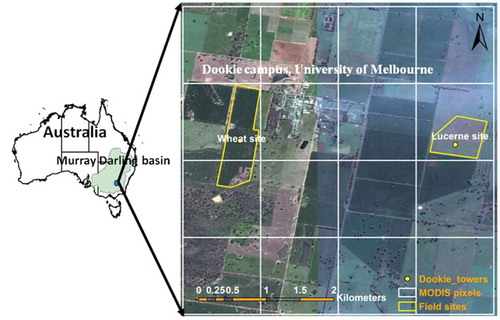
The experiment was conducted at the Dookie agriculture farm, at the University of Melbourne, Victoria, Australia. The climate is Mediterranean semi-arid with hot/dry summers and cold/wet winters (Bell, Eckard, and Cullen 2012). The experimental site is located in the southwest part of the Murray-Darling basin as shown, that practices rainfed agriculture. A meteorological tower was installed in a wheat site and data collected in 2012 and 2013 cropping seasons. Figure 1 shows the location of the Dookie experimental site in the Murray-Darling basin, Australia.

Figure 1. Location of the study area where the gridded overlay denotes MOSIS pixels

2.2. Dataset

Data collected from a wheat site for 2012 and 2013 cropping seasons has been used for model development. More details about the location and the study site is available in Akuraju et al. (2017). The “day of the year” is hereafter referred to as’DOY.’ Crops were sown on 15 May (DOY 136) and 24 May (DOY 144), respectively, in 2012 and 2013 seasons and were harvested on 9 December (DOY 344) and 7 December (DOY 357) each year (Akuraju et al. 2019). Soil moisture was recorded at average depths of 0–30 cm, 30–60 cm, 60–90 cm, and 90–120 cm using CS616 (Campbell Scientific, Inc.) water content reflectometers.

Ground-based surface temperature was measured using the thermal infrared radiometer (SI-111 manufactured by Apogee Inc.). The sensor measures the target temperature in the 8–14 µm atmospheric window. The surface temperature data was measured at 5-minute intervals and then averaged to produce 30-min interval data. The mid-day surface temperature data was used in this study to avoid the effect of intermittent clouds and changes in weather conditions. The ground-based mid-day surface temperature was assessed by comparing with MODIS 8 day 1-km resolution (MOD11A2).

As shown in Figure 2, the ground-based and MODIS surface temperature products show seasonal variations, where the maximum surface temperature was recorded in the dry summer period, and minimum temperature was recorded in the winter period. The correlation between ground-based and MODIS surface temperature was good throughout the cropping period, whereas ground-based measurements are high in the summer period as compared to MODIS measurements. However, this study only used the data in crop growing periods, so bias in the summer period will not affect the results. Overall, the ground-based surface temperature measurements were in good agreement with MODIS measurements with a Root Mean Squared Error (RMSE) of 1.5°C and R-squared (R²) value of 0.94 during cropping seasons.

Figure 2. (a) Comparison of ground-based and MODIS surface temperature.(b) Comparison of surface and air temperatures in 2012–2013 cropping seasons

The air temperature was measured using the HMP45C probe (Campbell Scientific, Inc.). Wind speed was measured using a 03101 R. M. Young (Campbell Scientific, Inc.) wind sentry set. CNR1 net radiometer (Kipp & Zonen, Inc.) was used to measure the net radiation. SKR-1850 and SKR-1870A light sensors (Skye Instruments Ltd, UK) were installed to measure the Normalized Difference Vegetation Index (NDVI). Crop height measured during our frequent visits to the study site was linearly interpolated to derive time series of canopy height.

2.3 Crop Water Stress Index (CWSI)

Monitoring differences between aerodynamic temperature (T_aero) estimates and air temperature (T_a) observations has been used to diagnose water stress in day time. Past studies (Kustas and Norman 1996) demonstrated that T_aero values have a complicated dependency on radiometric surface temperature (T_rad), vegetation characteristics and viewing angle. However, single source methods are encountered with problems where a partial vegetation cover exists in agriculture fields (Kustas et al. 1989; Vining and Blad 1992). To overcome this problem, the radiometric temperature is widely used for partitioning soil and canopy temperatures and heat fluxes in remote-sensing ET algorithms. Two-source energy balance methods divide the radiometric surface temperature into canopy temperature and soil temperature-based vegetation fraction visible at the thermal sensor’s view angle (Anderson et al. 2007).

This study used the Crop Water Stress Index (CWSI), which is based on the theoretical limits developed using canopy temperature and air temperature related to vapor pressure deficit (Jackson et al. 1981; Moran et al. 1994). The lower and upper bounds of canopy minus air temperature indicate non-water stressed and non-transpiring crop conditions that successfully related to crop yield and water requirements in a wheat field (Idso, Jackson, and Reginato 1977; Jackson, Reginato, and Idso 1977). It is assumed that when the crop transpires at a potential rate, the difference between a canopy and air temperature is small as the evaporated water cools the leaves. In water stress conditions, transpiration decreases with an increase in canopy temperature. The energy balance system for crop canopy is expressed as

(1) $R_n=LE+H+G$(1)

R_n is the net radiation (W/m²), LE is the latent heat flux (W/m²) and H is the sensible heat flux (W/m²) of the canopy. The complete and independent energy balance between the canopy and soil components of the surface is established. The sensible heat flux of the canopy can be expressed as:

(2) $H=\frac{\rho c_p\left(T_{aero}-T_a\right)}{r_a}$(2)

(3) $LE=\frac{\rho c_p\left(VPD\right)}{\gamma \left(r_a+r_c\right)}$(3)

ρ is the density of air (kg/m³), C_p is the heat capacity of air (J/kg/^oc), VPD is the vapor pressure deficit of the air, γ is the psychrometric constant (kpa/^oc), r_a is the aerodynamic resistance to heat transfer between the canopy and reference height (s/m), r_c is the canopy resistance (s/m), T_aero, and T_a are aerodynamic and air temperatures respectively.

Since aerodynamic temperature may not be measured directly using remote sensing, it is often replaced with radiometric or canopy temperature by adjusting aerodynamic and canopy resistances. The difference between radiometric temperature and the aerodynamic temperature is minimal and leads to small errors in heat flux predictions under dense vegetation conditions (Chehbouni et al. 1996; Sun and Mahrt 1995). Two-source models provide a more direct use of radiometric surface temperature over heterogeneous surfaces and reduce the errors associated with radiometer calibration, emissivity variations and use of temperature and wind speed data (Friedl 1996; Norman et al. 2000; Zhan, Kustas, and Humes 1996). In this study, canopy temperature is obtained from the Enhanced Two-source Evapotranspiration Model for Land (ETEML) method (Yang et al. 2015). This method is developed based on the theoretical VFC/LST trapezoid method, which decomposes composite radiometric surface temperature into canopy and soil temperatures.

It is assumed that a crop with adequate water supply transpires at a potential rate, and actual transpiration varies with the water availability for that crop. Hence, the ratio of actual to potential latent heat flux density indicates the crop water stress. The crop water stress index (CWSI) for the canopy can be expressed as follows:

(4) $CWSI=1-\frac{LE}{L{E}_p}=\frac{{\left(T_c-T_a\right)}_{min}-\left(T_c-T_a\right)}{{\left(T_c-T_a\right)}_{min}-{\left(T_c-T_a\right)}_{max}}$(4)

(T_c-T_a) is the difference between measured canopy and air temperature, (T_c-T_a) _min and (T_c-T_a) _max are the theoretical upper and lower limits of (T_c-T_a). The ratio of LE_c and LE_p ranges from 1 (ample water) to 0 (no available water). In general conditions, the plant goes from non-stress conditions to stress conditions that ranges from 0 to 1.

For the full canopy cover, G is negligible and the difference between canopy and air temperature by combining Equations (1)(1) $R_n=LE+H+G$(1) –(3(3) $LE=\frac{\rho c_p\left(VPD\right)}{\gamma \left(r_a+r_c\right)}$(3) ), which can be written as

(5) $T_c-T_a=\left[\frac{r_a{R}_n}{\rho c_p}\right]\left[\frac{\gamma \left(1+\frac{r_c}{r_a}\right)}{\left\{\mathrm{\Delta }+\gamma \left(1+\frac{r_c}{r_a}\right)\right\}}\right]-\frac{VPD}{\left\{\mathrm{\Delta }+\gamma \left(1+\frac{r_c}{r_a}\right)\right\}}$(5)

Theoretical crop water stress index (CWSI) can be derived using Equation (4)(4) $CWSI=1-\frac{LE}{L{E}_p}=\frac{{\left(T_c-T_a\right)}_{min}-\left(T_c-T_a\right)}{{\left(T_c-T_a\right)}_{min}-{\left(T_c-T_a\right)}_{max}}$(4) . In this approach, theoretical upper and lower limits of (T_c-T_a) were computed using Equation (5)(5) $T_c-T_a=\left[\frac{r_a{R}_n}{\rho c_p}\right]\left[\frac{\gamma \left(1+\frac{r_c}{r_a}\right)}{\left\{\mathrm{\Delta }+\gamma \left(1+\frac{r_c}{r_a}\right)\right\}}\right]-\frac{VPD}{\left\{\mathrm{\Delta }+\gamma \left(1+\frac{r_c}{r_a}\right)\right\}}$(5) . (T_c-T_a) _min is the lower bound of crop canopy-air temperature difference under well-watered vegetation conditions which can be expressed as:

(6) $(T_c-T_a{)}_{min}=\left[\frac{r_a{R}_n}{\rho c_p}\right]\left[\frac{\gamma \left(1+\frac{r_{cp}}{r_a}\right)}{\left\{\mathrm{\Delta }+\gamma \left(1+\frac{r_{cp}}{r_a}\right)\right\}}\right]-\frac{VPD}{\left\{\mathrm{\Delta }+\gamma \left(1+\frac{r_{cp}}{r_a}\right)\right\}}$(6)

r_cp is the canopy resistance (s/m) at potential evapotranspiration. For the full canopy cover with no available water, the upper bound of crop canopy-air temperature difference can be expressed as:

(7) $(T_c-T_a{)}_{max}=\left[\frac{r_a{R}_n}{\rho c_p}\right]\left[\frac{\gamma \left(1+\frac{r_{cx}}{r_a}\right)}{\left\{\mathrm{\Delta }+\gamma \left(1+\frac{r_{cx}}{r_a}\right)\right\}}\right]-\frac{VPD}{\left\{\mathrm{\Delta }+\gamma \left(1+\frac{r_{cx}}{r_a}\right)\right\}}$(7)

r_cx is the maximum canopy resistance (s/m) at complete stomata closure. Values of r_cp and r_cx can be derived using stomatal resistance (r_s) measurements and leaf area index (Monteith 1973).

(8) $r_{cp}=\frac{r_{sm}}{LAI}and{r}_{cx}=\frac{r_{sx}}{LAI}(LAI>0)$(8)

Values of r_cp and r_cx have also been published for many crops under different climatic conditions. If the values are not available, r_sm = 25–100 s/m and r_sx = 1000–1500 s/m would be reasonable values that would not result in appreciable errors in Equations (6(6) $(T_c-T_a{)}_{min}=\left[\frac{r_a{R}_n}{\rho c_p}\right]\left[\frac{\gamma \left(1+\frac{r_{cp}}{r_a}\right)}{\left\{\mathrm{\Delta }+\gamma \left(1+\frac{r_{cp}}{r_a}\right)\right\}}\right]-\frac{VPD}{\left\{\mathrm{\Delta }+\gamma \left(1+\frac{r_{cp}}{r_a}\right)\right\}}$(6) ) and (7(7) $(T_c-T_a{)}_{max}=\left[\frac{r_a{R}_n}{\rho c_p}\right]\left[\frac{\gamma \left(1+\frac{r_{cx}}{r_a}\right)}{\left\{\mathrm{\Delta }+\gamma \left(1+\frac{r_{cx}}{r_a}\right)\right\}}\right]-\frac{VPD}{\left\{\mathrm{\Delta }+\gamma \left(1+\frac{r_{cx}}{r_a}\right)\right\}}$(7) ).

Calculating the CWSI from Equation (4)(4) $CWSI=1-\frac{LE}{L{E}_p}=\frac{{\left(T_c-T_a\right)}_{min}-\left(T_c-T_a\right)}{{\left(T_c-T_a\right)}_{min}-{\left(T_c-T_a\right)}_{max}}$(4) requires maximum canopy resistance, minimum canopy resistance, canopy temperature, air temperature, net radiation, vapor pressure deficit and aerodynamic resistance. Accurate estimation of aerodynamic resistance is crucial for CWSI equations when it applies to different surface conditions. Aerodynamic resistance from highly stable conditions to unstable conditions (Brutsaert 1982) can be expressed as

(9) $r_a=\frac{\left[ln\left(\frac{z-d_o}{z_{om}}\right)+ln\left(\frac{z_{om}}{z_{oh}}\right)-{\psi }_h\right]\left[ln\left(\frac{z-d_o}{z_{om}}\right)-{\psi }_m\right]}{k^{2}U}$(9)

z is the height (m) of wind speed, and temperature measurements were made, d_o is displacement height (m/s), z_om and z_oh are roughness lengths for momentum and heat transfer, ψ_m, ψ_h are stability corrections for heat and momentum, k is von Karaman constant and U is wind speed (m/s).

In this method, theoretical lower and upper limits are functions of available energy, vapor pressure deficit, crop resistance, and aerodynamic resistance terms. Lower and upper baselines were created with knowledge of canopy and soil temperatures, which makes this model challenging to apply in practice. However, recent advances in remote sensing enabled us to decompose the surface temperature into soil temperature and canopy temperatures (Kustas and Norman 2000; Yang et al. 2015).

2.4 Available Water Fraction (AWF)

Soil moisture in the root-zone is dependent on soil type and horizons, and may not represent the water content available for transpiration. In this study, we used an alternate definition Available Water Fraction (AWF) to represent the root-zone soil moisture, which can be expressed as

(9) $AWF=\frac{\theta -{\theta }_{wp}}{{\theta }_{fc}-{\theta }_{wp}}$(9)

θ is measured soil moisture content, θ_wp and θ_fc are the soil moisture content at wilting point and field capacity respectively.

Soil moisture in the root-zone available for plants depends on soil water content and root distribution in the soil profile. The available water fraction in the root-zone was obtained based on the root distribution of the wheat crop. More details about root distribution and weighted root zone available water fraction is available in Akuraju et al. (2017). Hereafter, AWF is referred to as available water fraction in the root zone of 0–120 cm.

2.5 CWSI-AWF

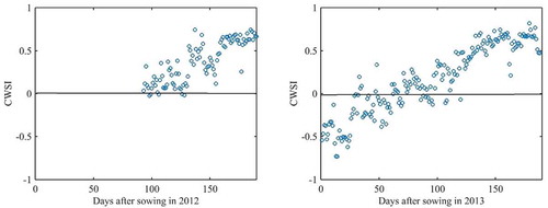
Theoretical CWSI was calculated using the data collected during 2012 (data collection started from 90 days after the wheat crop was sown) and 2013 cropping seasons in a wheat site. Following the equations in Sections 3 and 4, CWSI values were calculated using mid-day measurements. The relationship between CWSI and AWF is statistically significant in the 2012 and 2013 cropping seasons as shown in Figure 3. The scatter plot showed considerable variability in the CWSI-AWF relationship and evidence of nonlinear interactions in 2012 and linear interactions in 2013 cropping seasons. Regression analysis was performed for both cropping seasons and two different models were developed for 2012 and 2013 cropping seasons.

Figure 3. Crop water stress index values in (a) 2012 and (b) 2013 cropping season

For 2012 cropping season,

(10) $AWF=0.689\mathrm{e}\mathrm{x}\mathrm{p}\left(-3.225\ast CWSI\right)$(10)

And for 2013 cropping season,

(11) $AWF=\frac{0.5332-\mathrm{C}\mathrm{W}\mathrm{S}\mathrm{I}}{0.5783}$(11)

2.6 Net radiation

Net radiation is the crucial parameter for crop water demand and transpiration thus effects the non-water-stressed baseline of wheat crop. The correlation between CWSI and AWF can be compared to the errors associated with the subset of energy limited conditions. An important hypothesis here is that, beyond a certain threshold net radiation, there exists a strong relation between CWSI and AWF. Root mean square analysis and regression analysis were performed with different net radiation thresholds to evaluate the effect of net radiation on CWSI and AWF relationship (Section 3.2).

2.7 Cross validation

To develop a model that predicts root-zone soil moisture in both cropping seasons, models formulated in both cropping seasons were validated with another cropping season’s data. For this, AWF values were converted to volumetric soil moisture using wilting point and field capacity. In the first case, the model developed in the 2012 cropping season (non-linear model) was evaluated with 2013 observations. In the second case, the model developed in the 2013Table 1 cropping season (linear model) was validated with 2012 observations. Subsequent rows in Table 2 show the results of the 2013 cropping season.

Table 1. Statistics of root mean square error and coefficient of determination and number of samples in different net radiation thresholds. Values in bold are at critical threshold net radiation level

	2012			2013
Net radiation threshold	No. of samples	RMSE	R^2	No. of samples	RMSE	R^2
0	94	0.175	0.64	103	0.172	0.73
50	93	0.175	0.64	102	0.171	0.73
100	91	0.173	0.65	101	0.157	0.77
150	87	0.156	0.70	95	0.157	0.77
200	86	0.156	0.70	87	0.140	0.81
250	83	0.150	0.70	80	0.131	0.83
300	77	0.150	0.73	75	0.133	0.82
350	71	0.141	0.73	68	0.132	0.80
400	67	0.124	0.77	62	0.135	0.79
450	55	0.110	0.80	55	0.130	0.76
500	40	0.085	0.64	45	0.124	0.77
550	33	0.076	0.13	33	0.117	0.79
600	25	0.075	0.11	26	0.079	0.86

Table 2. Statistics of model calibration and cross-validation of models in different cropping seasons

Calibration	Evaluation	R	R^2	RMSE (%)	Bias (%)
2012	2012	0.85	0.70	3.9	−0.20
2013	2012	0.86	0.44	5.3	1.34
2013	2013	0.91	0.83	3.2	0.08
2012	2013	0.85	0.35	6.4	4.48

2.8 Model transferability

To evaluate the model’s applicability, the relation between CWSI and root-zone soil moisture was validated during three consecutive growing seasons (2002–04) at the USDA-ARS OPE³ experimental site. This section also validates the usefulness of the root-zone soil moisture model developed using the 2013 Dookie dataset from the USDA experimental site. The corn crop was sown in the experimental site and the length of the cropping season was different in different years. This site is a well-known site for its continuous availability of root-zone soil moisture and the development of remote sensing based root-zone soil moisture algorithms (Crow, Kustas, and Prueger 2008; Li, Crow, and Kustas 2010b). Details of the study site and cropping seasons can be found in Li, Crow, and Kustas (2010b). All meteorological datasets were collected from sowing to harvesting period of the crop. Daily time series of land surface temperature and NDVI dataset has been created by linearly interpolated MODIS 8-day 1-km Land surface temperature (MOD11A2), MODIS 16-day 250-m NDVI (MOD13Q1) products during the experimental period.

Profile soil moisture measurements collected in 10, 30, 50 and 80 cm depths in the OPE³ site and top 1 m vertically integrated root-zone soil moisture is obtained by averaging the measurements. The USDA supplies soil moisture data that is presented here in the form of m³/m³. The RZSM varies from 0.06 to 0.29 m³/m³ during the 2002–2004 cropping seasons.

Before estimating RZSM in the OPE³ site, the maximum and minimum soil moisture values were considered as field capacity and wilting point of that soil. These values can also be obtained from the Handbook of Hydrology (Maidment 1993) with knowledge of soil type. The available water fraction in root-zone soil moisture was obtained by using Equation 11(11) $AWF=\frac{0.5332-\mathrm{C}\mathrm{W}\mathrm{S}\mathrm{I}}{0.5783}$(11) . Volumetric root-zone soil moisture values were obtained by rearranging **Equation for model validation.

2.9 MODIS data

Predicted root-zone soil moisture from the model is validated at the MODIS pixel level. Annual time series of LST was extracted from 1-km MODIS Land Surface Temperature and Emissivity Daily L3 Global version 4.1 (MOD11A1). Since the experimental site was located within two pixels, the pixel that included the most cropping area was used for analysis. CWSI was calculated from MODIS TIR data and meteorological data collected from the experimental site. AWF in the root zone obtained from the model has been converted to soil moisture using field capacity and wilting point.

3. Results and discussion

3.1 Model evaluation

Theoretical CWSI values were calculated using the method described in Section 2.3. As shown in Figure 3, CWSI values in the 2012 and 2013 cropping seasons are below zero representing the theoretical lower limit of non-water stress conditions. Aerodynamic resistance values are directly dependent on the roughness length of the crop. Therefore, canopy height would influence CWSI values because it affects the zero plane displacement and roughness length. Roughness length, together with wind speed influence aerodynamic resistance of crops and the ratio of r_c/r_a. Aerodynamic resistance values derived from **Equation) were greater than 100 s/m in initial crop growth stages. Most CWSI values are below zero in initial crop growth stages as shown in Figure 3 due to low or no vegetation. In partial vegetative cover conditions, the CWSI values do not represent the true crop water stress status (as an indicator of root-zone soil moisture content) since the soil temperature may heavily influence the aggregated temperature at the satellite pixel scale. Rather, the index is likely associated with the soil surface wetness in initial crop growth stages. Also, CWSI values are below zero when assumed potential canopy resistance values are too high. Canopy resistance values of minimum (50 s/m) and maximum values (1100 s/m) were used in this study to adjust the non-water-stressed baseline (Jackson et al. 1981; Wanjura, Hatfield, and Upchurch 1990).

Direct use of surface temperature in CWSI calculations is prone to large errors due to soil cover and visibility (Jones et al. 2009; Tilling et al. 2007). To avoid confounding canopy temperature measurements with the influence of the soil background, this study only used the data collected during periods when the soil surface was not exposed. For instance, only data collected 90 days after the crop sown in the 2012 cropping season were included in this study. The crop canopy is visually inspected from daily photographs taken using the camera installed on the meteorological tower. Results obtained from Enhanced Two-source Evapotranspiration Model for Land (ETEML) method (Yang et al. 2015) was also indicated that decomposition of surface temperature into canopy temperature and soil temperature after 90 days of the crop growing season.

The relationship between CWSI and AWF appeared to be constrained by AWF in the mid-growth and harvesting stages. As shown in Figure 4, AWF values moved from right to left representing soil moisture values near the field capacity in the mid-growth stage reaching wilting point in the crop harvesting stage in both cropping seasons. CWSI values are moving from 0 to 0.8 representing non-water stress conditions in mid-growth stages to water stress conditions in the harvesting stage.

Figure 4. Relationship between AWF in the root zone and CWSI with the color of points represents the days after sowing. (a) AWF vs. CWSI in 2012; (b) AWF vs. CWSI in 2013

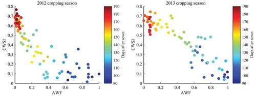
The variability of soil moisture stress function CWSI-AWF can be explained by rainfall variability and available soil moisture in both cropping seasons (Akuraju et al. 2017). Results showed that low rainfall distribution in the 2012 cropping season led to an AWF that was less than 0.3 in most number of days. This situation also represents water stress conditions of the wheat crop in the 2012 cropping season. In contrast, wheat crop went from non-water stress conditions to stress conditions as there was enough soil moisture available throughout the 2013 cropping season. This situation represented the negative linear relationship between CWSI and AWF in 2013.

3.2 Effect of net radiation

Another potential parameter that may affect the non-water-stressed baseline of wheat is net radiation. The effect of net radiation on the relationship between CWSI and root-zone soil moisture in two cropping seasons was analyzed. This analysis was performed to identify a critical net radiation threshold level in order to develop a regression model for both the cropping seasons. The net radiation ranges from 0 to 600 W/m² in the experimental period divided into 50 W/m² increments to obtain an RMSE. The coefficient of determination at each threshold level is presented in Table 1. Analysis indicated that RMSE values are continuously decreasing from 0.175 to 0.15 in 2012 and 0.172 to 0.131 in 2013 cropping seasons, until the net radiation threshold value of 250 W/m².

Results also indicated that the correlation (measured using the coefficient of determination) increased with an increase in net radiation threshold levels (R² value increases from 0.64 to 0.80) until 400 W/m² and correlation decreased after this net radiation threshold in the 2012 cropping season. Increase in correlation excluding scattered points from the mid-growth stage and decrease in correlation arose due to a considerable reduction in a number of samples. In the 2013 cropping season, correlation values increased from 0.73 to 0.83 until 250 W/m² and decreased thereafter excluding a number of samples. The 2013 cropping season results showed high correlation and low RMSE values beyond a critical threshold level of 250 W/m². The model performance increased after the critical threshold net radiation level of 250 W/m² in the 2012 cropping season led to a substantial reduction in the number of samples. Based on variation in RMSE and R² values from two cropping seasons at different net radiation thresholds, it was noted that the net radiation 250 W/m² is a critical threshold level that is influencing the relation between CWSI and AWF. To avoid the errors associated with low available energy, net radiation values less than 250 W/m² were excluded from the analysis.

3.3 Model validation

3.3.1 Cross validation

To develop a model that predicts root-zone soil moisture in both cropping seasons, models formulated in both cropping seasons were validated with another cropping season’s data. Cross-validation errors are not directly comparable with limited data points. Relative accuracy of 2012 and 2013 models cannot be judged without sufficiently large data sets; so a bootstrap method was used to identify the model RMSE of each calibrated model so as to predict the root-zone soil moisture in another cropping season.

The bootstrapping method (Efron 1979) was initiated by resampling the data set 10,000 times to generate random data sets. The RMSE is chosen to evaluate the model performance, and the accuracy of each sample is calculated. The histogram of RMSE in two cropping seasons is shown in Figure 5.

Figure 5. Histogram showing the frequency distribution of RMSE derived from bootstrapping method: (a) 2013 model validated in 2012 cropping season. (b) 2012 model validated in 2013 cropping season

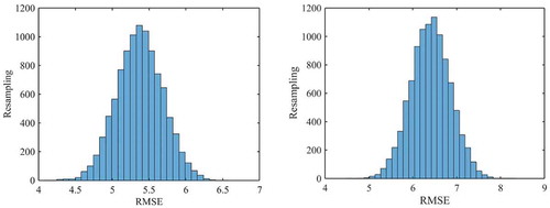
Error frequency histogram results demonstrate the results obtained from the bootstrapping method. The linear model predicted the RZSM with a minimum accuracy of 4% and a maximum of 6.5% when resampled from the 2012 cropping season data. The peak histogram value indicated that the model predicted RZSM with an accuracy of 5.4% from most of the samples. Likewise, the non-linear model predicted the RZSM with an accuracy of 6.4% from most of the samples from the 2013 cropping season. Using this analysis, the linear model appears to be more representative between CWSI and AWF, exhibiting the smallest RMSE in both cropping seasons.

CWSI values were calculated using the equations in Section 2.3. The analysis showed good agreement between observed and predicted root-zone soil moisture representing the model performance of the calibrated models. Cross-validation results showed that the non-linear model estimated root-zone soil moisture with an RMSE of 6.4% and an R² value of 0.35 in the 2013 cropping season. Better root-zone soil moisture values were obtained in the 2012 cropping season using a linear model with an RMSE of 5.3% and an R² value of 0.44.

3.3.2 Validation at OPE³ site

To evaluate the applicability of the developed model with OPE³ dataset at the USDA experimental site. Figure 6(a) shows that there is a negative correlation between CWSI and RZSM in the 2002 cropping season. A similar correlation was obtained between CWSI and RZSM in the 2004 cropping season. AWF values were moved from right to left, representing soil moisture values near to field capacity in the mid-growth stage reaching a wilting point at the crop’s harvesting stage. Overall, the correlation between CWSI and RZSM is similar to the correlation obtained from the Dookie wheat site. However, the correlation between CWSI and RZSM in the 2003 cropping season is not statistically significant because of high soil moisture availability in the root zone compared to the 2002 and 2004 cropping seasons. RZSM values varied from 0.12 to 0.24 m³/m³ during the 2003 cropping period, which led to poor correlation.

Figure 6. (a) Correlation between CWSI and root-zone soil moisture in OPE³ site. (b) Correlation of observed vs. model predicted root-zone soil moisture

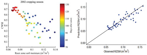
Retrievals of root-zone zone soil moisture from a linear model were compared to observations in three cropping seasons at the OPE³ site. Statistical metrics of R, R², RMSE and bias are listed in Table 3 to examine the RZSM model’s accuracy. The linear model performs best, exhibiting the smallest RMSE and highest correlation with an R² value of 0.77 and an RMSE of 3.77 in the 2002 cropping season. In the 2003 cropping season, the model yielded larger errors with an R² value of 0.20 and an RMSE of 4.80. Large errors in RZSM estimations occurred due to non-stress conditions in the 2003 cropping season. In this period, most of the CWSI values were close to 0.2 representing non-water stress conditions because of soil moisture near field capacity.

Table 3. Model performance in three cropping seasons at the OPE³ site

Cropping season	R	R^2	RMSE	Bias
2002	0.82	0.77	3.77	3.78
2003	0.61	0.20	4.80	2.61
2004	0.74	0.45	1.68	1.18

The distribution of predicted and observed RZSM values in the 2004 cropping season also exhibits the best performance with an R² value of 0.45 and an RMSE of 1.68. The linear model yielded a smaller bias in root-zone soil moisture estimations over three cropping seasons as shown in Table 3. Overall, the linear model provided the best performance under water stress conditions at the OPE³ site.

3.3.3 Validation at a pixel level

Root-zone soil moisture derived from a linear model is validated at MODIS pixel level. Retrievals of root-zone soil moisture were compared to observations from 2012 and 2013 cropping seasons and listed in Table 4. The bias between modeled and measured root-zone soil moisture values were 0.45 m³/m³ and 2.45 m³/m³ in the 2012 and 2013 cropping seasons. A good agreement was found between the TIR-based root-zone soil moisture retrievals and observations from the Dookie experimental site using the linear model. This suggests the efficacy of TIR data in root-zone soil moisture estimations.

Table 4. Model performance at MODIS pixel level

Cropping season	R	R^2	RMSE	Bias
2012	0.50	0.38	7.3	0.45
2013	0.69	0.42	6.4	2.05

It should also be noted that the linear model developed using data collected in the 2013 cropping season provided better performance in both cropping seasons. Validation of the linear model also suggested that the model has the potential to estimate root-zone soil moisture in water stress conditions at the OPE³ site. Comparison with MODIS-based root-zone soil moisture retrievals showed the TIR-based model’s feasibility at a regional scale. The model validation is limited with the availability of continuous root-zone soil moisture data in a cropping season. Overall, the results suggest that the model is a promising tool to estimate root-zone soil moisture.

Results indicated that the model could perform well when AWF conditions are between field capacity and wilting point. Beyond this condition, the model may not capture root-zone soil moisture accurately. CWSI developed in this study is dependent on the energy exchanges between soil, vegetation and atmosphere; thus it depends on sensible heat flux, canopy, air temperature and resistances. If the soil is above field capacity and beyond the wilting point, the energy exchange with the atmosphere is negligible. In these conditions, canopy transpiration and soil evaporation cannot be related separately to canopy and soil temperatures. Frequently changing climatic conditions often lead to large errors. For example, air temperature measurements before or after canopy temperature measurements in rapidly changing cloud conditions lead to huge errors, which is also mentioned in Jackson et al. (1981).

According to the present results and concerning the root-zone soil moisture validation strategies, additional reliable datasets are required to validate the model. For example, under some particular agro-ecological conditions, vegetation types, geographical areas where the estimates were frequently affected by clouds, reliable soil moisture estimates were possible using thermal infrared remote sensing. Moreover, since no satellite sensors measure root-zone soil moisture explicitly, in-situ root-zone soil moisture measurements from reliable monitoring networks can be employed to calibrate the model. Due to the low availability of thermal infrared data at high temporal and spatial resolutions, developing a reliable method for extrapolating daily values to longer time scales is essential.

4. Conclusions

This study has shown that the canopy temperature based Crop Water Stress Index model can provide valuable information on root-zone soil moisture. CWSI values ranging from 0 to 0.8 represent non-water stress conditions in mid-growth stages to water stress conditions in the harvesting stage at the experimental site. The sources of errors could be avoided by excluding initial crop growth stages and assuming high potential canopy resistance values. Results also showed that low net radiation days (net radiation less than 250 W/m²) decrease the accuracy of root zone soil moisture estimations. Two empirical models were developed to estimate root-zone soil moisture from two cropping seasons in a wheat site. Cross-validation results showed that the linear model that was developed is reasonably well-performing in both cropping seasons. Validation results from the OPE³ site announce that CWSI is a promising tool to estimate RZSM from two cropping seasons in a corn site. However, the prediction accuracy of RZSM also depends on moisture availability and the number of samples. For instance, high root-mean-square-errors were observed in the 2003 cropping season due to high soil moisture conditions. Thus, the empirical CWSI model is an efficient approach for root-zone soil moisture estimations when the crop reaches its full canopy cover.

Acknowledgements

The authors would like to thank the Australian Centre for International Agriculture Research (ACIAR) for sponsoring the research under the John Allwright Fellowship. The authors gratefully acknowledge the support received from Robert Pipunic and Rodger Ian Young in data collection in Dookie experimental site. We are also thankful to USDA-ARS Hydrology and Remote Sensing Laboratory for providing the extensive OPE³ dataset.

Disclosure statement

No potential conflict of interest was reported by the authors.

References

- Akuraju, V. R., D. Ryu, B. George, Y. Ryu, and K. Dassanayake. 2013. “Analysis of Root-zone Soil Moisture Control on Evapotranspiration in Two Agriculture Fields in Australia.” In MODSIM2013, 20th International Congress on Modelling and Simulation, edited by J. In Piantadosi, R. S. Anderssen, and J. Boland. Adelaide: Modelling and Simulation Society of Australia and New Zealand.
- Akuraju, V. R., D. Ryu, B. George, Y. Ryu, and K. Dassanayake. 2017. “Seasonal and Inter-annual Variability of Soil Moisture Stress Function in Dryland Wheat Field, Australia.” Agricultural and Forest Meteorology 232: 489–499. doi:10.1016/j.agrformet.2016.10.007.
- Akuraju, V. R., D. Ryu, A. W. Western, and R. Ian Young. 2019. “Towards Estimating Root-zone Soil Moisture Using Surface Multispectral and Thermal Sensing: A Spectral and Hydrometeorological Dataset from the Dookie Experiment Site, Victoria, Australia.” Hydrological Processes 33 (14): 2037–2043. doi:10.1002/hyp.13459.
- Anderson, M. C., J. M. Norman, J. R. Mecikalski, J. A. Otkin, and W. P. Kustas. 2007. “A Climatological Study of Evapotranspiration and Moisture Stress across the Continental United States Based on Thermal Remote Sensing: 1. Model Formulation.” Journal of Geophysical Research-Atmospheres 112: D10. doi:10.1029/2006jd007506.
- Bell, M. J., R. J. Eckard, and B. R. Cullen. 2012. “The Effect of Future Climate Scenarios on the Balance between Productivity and Greenhouse Gas Emissions from Sheep Grazing Systems.” Livestock Science 147 (1–3): 126–138. doi:10.1016/j.livsci.2012.04.012.
- Brutsaert, W. 1982. Evaporation into the Atmosphere: Theory, History, and Applications. New york: Springer.
- Calvet, J., J.-P. Wigneron, J. Walker, F. Karbou, A. Chanzy, C. Albergel. 2011. “Sensitivity of Passive Microwave Observations to Soil Moisture and Vegetation Water Content: L-Band to W-Band.” IEEE Transactions on Geoscience and Remote Sensing 49 (4): 1190–1199. doi:10.1109/TGRS.2010.2050488.
- Carlson, T. N., J. K. Dodd, S. G. Benjamin, and J. N. Cooper. 1981. “Satellite Estimation of the Surface-Energy Balance, Moisture Availability and Thermal Inertia.” Journal of Applied Meteorology 20 (1): 67–87. doi:10.1175/1520-0450(1981)020<0067:Seotse>2.0.Co;2.
- Chehbouni, A., D. Lo Seen, E. G. Njoku, and B. M. Monteny. 1996. “Examination of the Difference between Radiative and Aerodynamic Surface Temperatures over Sparsely Vegetated Surfaces. Remote Sens.” Environ. 58 (2): 177–186. doi:10.1016/S0034-4257(96)00037-5.
- Crago, R. D. 1996a. “Comparison of the Evaporative Fraction and the Priestley-Taylor Alpha for Parameterizing Daytime Evaporation.” Water Resources Research 32 (5): 1403–1409. doi:10.1029/96wr00269.
- Crow, W. T., and W. P. Kustas. 2005. “Utility of Assimilating Surface Radiometric Temperature Observations for Evaporative Fraction and Heat Transfer Coefficient Retrieval.” Boundary-Layer Meteorology 115 (1): 105–130. doi:10.1007/s10546-004-2121-0.
- Crow, W. T., W. P. Kustas, and J. H. Prueger. 2006. “Monitoring Root-zone Soil Moisture through the Assimilation of a Thermal Remote Sensing-based Soil Moisture Proxy into a Water Balance Model.” Remote Sensing of Environment 112: 1268–1281. doi:10.1016/j.rse.2006.11.033.
- Crow, W. T., W. P. Kustas, and J. H. Prueger. 2008. “Monitoring Root-zone Soil Moisture through the Assimilation of a Thermal Remote Sensing-based Soil Moisture Proxy into a Water Balance Model.” Remote Sensing of Environment 112 (4): 1268–1281. doi:10.1016/j.rse.2006.11.033.
- Dabrowska-Zielinska, K., J. Musial, A. Malinska, M. Budzynska, R. Gurdak, W. Kiryla, M. Bartold, et al. 2018. “Soil Moisture in the Biebrza Wetlands Retrieved from Sentinel-1 Imagery.” Remote Sensing 10 (12). doi:10.3390/rs10121979.
- Das, N. N., and B. P. Mohanty. 2006. “Root Zone Soil Moisture Assessment Using Remote Sensing and Vadose Zone Modeling.” Vadose Zone Journal 5 (1): 296–307. doi:10.2136/Vzj2005.0033.
- Davies, J. A. 1972. “Actual, Potential and Equilibrium Evaporation for a Beanfield in Southern Ontario.” Agricultural Meteorology 10 (4–5): 331-+. doi:10.1016/0002-1571(72)90036-2.
- Dorigo, W. A., W. Wagner, R. Hohensinn, S. Hahn, C. Paulik, A. Xaver, A. Gruber, et al. 2011. “The International Soil Moisture Network: A Data Hosting Facility for Global in Situ Soil Moisture Measurements.” Hydrology and Earth System Sciences 15 (5): 1675–1698. doi:10.5194/hess-15-1675-2011.
- Efron, B. 1979. “Bootstrap Methods - Another Look at the Jackknife.” Annals of Statistics 7 (1): 1–26. doi:10.1214/aos/1176344552.
- El Hajj, M., N. Baghdadi, M. Zribi, G. Belaud, B. Cheviron, D. Courault, F. Charron, et al. 2016. “Soil Moisture Retrieval over Irrigated Grassland Using X-band SAR Data.” Remote Sensing of Environment 176 :202–218. doi:10.1016/j.rse.2016.01.027.
- Engman,, and C. Narinder. 1995. “Status of Microwave Soil Moisture Measurements with Remote Sensing.” Remote Sensing of Environment 51: 189–198. doi:10.1016/0034-4257(94)00074-w.
- Entekhabi, D., H. Nakamura, and E. G. Njoku. 1994. “Solving the Inverse Problems for Soil-Moisture and Temperature Profiles by Sequential Assimilation of Multifrequency Remotely-Sensed Observations.” IEEE Transactions on Geoscience and Remote Sensing 32 (2). doi:10.1109/36.295058.
- Friedl, M. A. 1996. “Relationships among Remotely Sensed Data, Surface Energy Balance, and Area-averaged Fluxes over Partially Vegetated Land Surfaces.” Journal of Applied Meteorology 35 (11): 2091–2103. doi:10.1175/1520-0450(1996)035<2091:Rarsds>2.0.Co;2.
- Gao, B.-C. 1996. “NDWI—A Normalized Difference Water Index for Remote Sensing of Vegetation Liquid Water from Space.” Remote Sensing of Environment 58 (3): 257–266. doi:10.1016/S0034-4257(96)00067-3.
- Gentine, P., D. Entekhabi, A. Chehbouni, G. Boulet, and B. Duchemin. 2007. “Analysis of Evaporative Fraction Diurnal Behaviour.” Agricultural and Forest Meteorology 143 (1–2): 13–29. doi:10.1016/j.agrformet.2006.11.002.
- Gu, Y., E. Hunt, B. Wardlow, J. B. Basara, J. F. Brown, J. P. Verdin. 2008. “Evaluation of MODIS NDVI and NDWI for Vegetation Drought Monitoring Using Oklahoma Mesonet Soil Moisture Data.” Geophysical Research Letters 35 (22). doi:10.1029/2008GL035772.
- Hain, C. R., W. T. Crow, M. C. Anderson, and J. R. Mecikalski. 2012. “An Ensemble Kalman Filter Dual Assimilation of Thermal Infrared and Microwave Satellite Observations of Soil Moisture into the Noah Land Surface Model.” Water Resources Research 48. doi:10.1029/2011wr011268.
- Hain, C. R., W. T. Crow, J. R. Mecikalski, M. C. Anderson, and T. Holmes. 2011. “An Intercomparison of Available Soil Moisture Estimates from Thermal Infrared and Passive Microwave Remote Sensing and Land Surface Modeling.” Journal of Geophysical Research-Atmospheres 116. doi:10.1029/2011jd015633.
- Hain, C. R., J. R. Mecikalski, and M. C. Anderson. 2009. “Retrieval of an Available Water-Based Soil Moisture Proxy from Thermal Infrared Remote Sensing. Part I: Methodology and Validation.” Journal of Hydrometeorology 10 (3): 665–683. doi:10.1175/2008jhm1024.1.
- Idso, S. B., R. D. Jackson, and R. J. Reginato. 1977. “Remote-Sensing of Crop Yields.” Science 196 (4285): 19–25. doi:10.1126/science.196.4285.19.
- Jackson, R. D., S. B. Idso, R. J. Reginato, and P. J. Pinter. 1981. “Canopy Temperature as a Crop Water-Stress Indicator.” Water Resources Research 17 (4): 1133–1138. doi:10.1029/WR017i004p01133.
- Jackson, R. D., R. J. Reginato, and S. B. Idso. 1977. “Wheat Canopy Temperature - Practical Tool for Evaluating Water Requirements.” Water Resources Research 13 (3): 651–656. doi:10.1029/WR013i003p00651.
- Jones, H. G., R. Serraj, B. R. Loveys, L. Xiong, A. Wheaton, A. H. Price. 2009. “Thermal Infrared Imaging of Crop Canopies for the Remote Diagnosis and Quantification of Plant Responses to Water Stress in the Field.” Functional Plant Biology : FPB 36 (11): 978–989. doi:10.1071/FP09123.
- Kustas, W. P., B. J. Choudhury, M. S. Moran, R. J. Reginato, R. D. Jackson, L. W. Gay, H. L. Weaver, et al. 1989. “Determination of Sensible Heat Flux over Sparse Canopy Using Thermal Infrared Data.” Agricultural and Forest Meteorology 44 (3): 197–216. doi:10.1016/0168-1923(89)90017-8.
- Kustas, W. P., and J. M. Norman. 1996. “Use of Remote Sensing for Evapotranspiration Monitoring over Land Surfaces.” Hydrological Sciences Journal 41 (4): 495–516. doi:10.1080/02626669609491522.
- Kustas, W. P., and J. M. Norman. 2000. “A Two-Source Energy Balance Approach Using Directional Radiometric Temperature Observations for Sparse Canopy Covered Surfaces.” Agronomy Journal 92 (5): 847–854. doi:10.2134/agronj2000.925847x.
- Li, F. Q., W. T. Crow, and W. P. Kustas. 2010a. “Towards the Estimation Root-zone Soil Moisture via the Simultaneous Assimilation of Thermal and Microwave Soil Moisture Retrievals.” Advances in Water Resources 33 (2): 201–214. doi:10.1016/j.advwatres.2009.11.007.
- Li, F. Q., W. T. Crow, and W. P. Kustas. 2010b. “Towards the Estimation Root-zone Soil Moisture via the Simultaneous Assimilation of Thermal and Microwave Soil Moisture Retrievals.” Advances in Water Resources 33 (2): 201–214. doi:10.1016/j.advwatres.2009.11.007.
- Maidment, D. R. 1993. Handbook of Hydrology. New York: McGraw-Hill.
- Monteith, J. 1973. Principles of Environmental Physics. London: Edward Arnold.
- Moran, M. S., T. R. Clarke, Y. Inoue, and A. Vidal. 1994. “Estimating Crop Water Deficit Using the Relation between Surface-air Temperature and Spectral Vegetation Index.” Remote Sensing of Environment 49 (3): 246–263. doi:10.1016/0034-4257(94)90020-5.
- Njoku, E. G., and L. Li. 1999. “Retrieval of Land Surface Parameters Using Passive Microwave Measurements at 6-18 GHz.” IEEE Transactions on Geoscience and Remote Sensing 37 (1): 79–93. doi:10.1109/36.739125.
- Norman, J. M., W. P. Kustas, and K. S. Humes. 1995. “Source Approach for Estimating Soil and Vegetation Energy Fluxes in Observations of Directional Radiometric Surface-Temperature.” Agricultural and Forest Meteorology 77: 3–4. doi:10.1016/0168-1923(95)02265-Y.
- Norman, J. M., W. P. Kustas, J. H. Prueger, and G. R. Diak. 2000. “Surface Flux Estimation Using Radiometric Temperature: A Dual Temperature-difference Method to Minimize Measurement Errors.” Water Resources Research 36 (8): 2263–2274. doi:10.1029/2000wr900033.
- Paloscia, S., G. Macelloni, P. Pampaloni, R. Ruisi, and E. Santi, 2001. “CHEERS Experiment in Tuscany: A Comparison between L- Band and C- and X-Bands Capability in Measuring Soil Moisture.” In IEEE International Geoscience and Remote Sensing Symposium, I: 22–24. USA. doi:10.1109/IGARSS.2001.976045.
- Paltineanu, C., E. Chitu, and N. Tanasescu. 2011. “Correlation between the Crop Water Stress Index and Soil Moisture Content for Apple in a Loamy Soil: A Case Study in Southern Romania.” Vi International Symposium on Irrigation of Horticultural Crops 889: 257–264.
- Rahimzadeh-Bajgiran, P., A. A. Berg, C. Champagne, and K. Omasa. 2013. “Estimation of Soil Moisture Using Optical/thermal Infrared Remote Sensing in the Canadian Prairies.” Isprs Journal of Photogrammetry and Remote Sensing 83: 94–103. doi:10.1016/j.isprsjprs.2013.06.004.
- Sabater, J. M., L. Jarlan, J. C. Calvet, F. Bouyssel, and P. De Rosnay. 2007. “From Near-surface to Root-zone Soil Moisture Using Different Assimilation Techniques.” Journal of Hydrometeorology 8 (2): 194–206. doi:10.1175/Jhm571.1.
- Schmugge, T. J. 1985. Remote Sensing of Soil Moisture. Hydrological Forecasting. New York: Wiley. doi:10.1155/2013/424178.
- Schmugge, T. J., J. R. Wang, and G. Asrar. 1988. “Results from the Push Broom Microwave Radiometer Flights over the Konza Prairie in 1985.” IEEE Transactions on Geoscience and Remote Sensing 26: 590–596. doi:10.1109/36.7684.
- Scott, C. A., W. G. M. Bastiaanssen, and M. U. D. Ahmad. 2003. “Mapping Root Zone Soil Moisture Using Remotely Sensed Optical Imagery.” Journal of Irrigation and Drainage Engineering-ASCE 129 (5): 326–335. doi:10.1061/(ASCE)0733-9437(2003)129:5(326).
- Sun, J., and L. Mahrt. 1995. “Determination of Surface Fluxes from the Surface Radiative Temperature.” Journal of the Atmospheric Sciences 52 (8): 1096–1106. doi:10.1175/1520-0469(1995)052<1096:dosfft>2.0.co;2.
- Tilling, A. K., G. J. O’Leary, J. G. Ferwerda, S. D. Jones, G. J. Fitzgerald, D. Rodriguez, R. Belford, et al. 2007. “Remote Sensing of Nitrogen and Water Stress in Wheat.” Field Crops Research 104 (1–3): 77–85. doi:10.1016/j.fcr.2007.03.023.
- Vining, R. C., and B. L. Blad. 1992. “Estimation of Sensible Heat Flux from Remotely Sensed Canopy Temperatures.” Journal of Geophysical Research: Atmospheres 97 (D17): 18951–18954. doi:10.1029/92JD01626.
- Wang, J. R., J. C. Shiue, and J. E. Mcmurtrey. 1980. “Microwave Remote-Sensing of Soil-Moisture Content over Bare and Vegetated Fields. Geophys.” Geophysical Research Letters 7 (10): 801–804. doi:10.1029/GL007i010p00801.
- Wang, L., and J. J. Qu. 2007. “NMDI: A Normalized Multi-band Drought Index for Monitoring Soil and Vegetation Moisture with Satellite Remote Sensing.” Geophysical Research Letters 34 (20). doi:10.1029/2007GL031021.
- Wang, X. W., H. J. Xie, H. D. Guan, and X. B. Zhou. 2007. “Different Responses of MODIS-derived NDVI to Root-zone Soil Moisture in Semi-arid and Humid Regions.” Journal of Hydrology 340 (1–2): 12–24. doi:10.1016/j.jhydrol.2007.03.022.
- Wanjura, D. F., J. L. Hatfield, and D. R. Upchurch. 1990. “Crop Water-Stress Index Relationships with Crop Productivity.” Irrigation Science 11 (2): 93–99. doi:10.1007/BF00188445.
- Western, A. W., R. B. Grayson, and G. Bloschl. 2002. “Scaling of Soil Moisture: A Hydrologic Perspective.” Annual Review of Earth and Planetary Sciences 30 (1): 149. doi:10.1146/annurev.earth.30.091201.140434.
- Wheaton, A. D., et al. 2011. “Use of Thermal Imagery to Detect Water Stress during Berry Ripening in Vitis Vinifera L. ‘Cabernet Sauvignon’.” Vi International Symposium on Irrigation of Horticultural Crops 889: 123–130.
- Yang, Y., H. Su, R. Zhang, J. Tian, and L. Li. 2015. “An Enhanced Two-source Evapotranspiration Model for Land (ETEML): Algorithm and Evaluation.” Remote Sensing of Environment 168: 54–65. doi:10.1016/j.rse.2015.06.020.
- Zhan, X., W. P. Kustas, and K. S. Humes. 1996. “An Intercomparison Study on Models of Sensible Heat Flux over Partial Canopy Surfaces with Remotely Sensed Surface Temperature.” Remote Sensing of Environment 58 (3): 242–256. doi:10.1016/S0034-4257(96)00049-1.