Investigating different versions of PROSPECT and PROSAIL for estimating spectral and biophysical properties of photosynthetic and non-photosynthetic vegetation in mixed grasslands

ABSTRACT

The PROSPECT and PROSAIL family of radiative transfer models (RTMs) are among the most popular for simulating vegetation spectra and estimating vegetation properties at the leaf and canopy levels. However, the main limitation of the radiative transfer model approach is that model performance depends on the exhaustiveness of the calibration database(s). The PROSPECT model was calibrated mainly with photosynthetic leaves, and thus does not contain specific absorption coefficients of decay pigments responsible for the spectral behavior of non-photosynthetic vegetation. Hence, PROSPECT and PROSAIL may be ill-suited to mixed ecosystems (e.g., grasslands and wetlands), especially in the late growing season when the non-photosynthetic vegetation is likely to obfuscate the quantification of green vegetation. This study investigates the performance of different versions of PROSPECT/PROSAIL models for simulating spectra and estimating biophysical properties of photosynthetic and non-photosynthetic vegetation, and aims to better understand the limitations of these RTMs and identify possible ways to improve their performance. Results show that the PROSPECT-5 and PROSPECT-D had challenges in simulating spectra of non-photosynthetic leaves in a mixed grassland area, while a modified version (PROSPECT-5M) that considered the absorption effects of decay pigments achieved higher accuracy (e.g., mean Root Mean Square Error (RMSE) of 0.014 compared to 0.026 for the PROSPECT-5). In comparison, there is minimal difference in RMSE between models for simulating green photosynthetic leaves. At the canopy level, the original PROSAIL model simulated the spectra well for homogeneous green canopies (with mean RMSE around 0.012), while a modified PROSAIL model simulated the spectra more accurately for mixed canopies that have photosynthetic and non-photosynthetic leaves (e.g., with a mean RMSE of 0.010 compared to 0.020 of original PROSAIL). The original and modified PROSAIL were then inverted using helicopter-based high-spatial resolution hyperspectral imagery to estimate vegetation properties, and achieved higher accuracies for green and mixed canopies, respectively (e.g., estimating canopy chlorophyll with R² values over 0.75). Overall, different versions of PROSPECT/PROSAIL models have a varied performance for photosynthetic and non-photosynthetic vegetation. Understanding the limitations of the models and adopting corresponding measures to improve their performance is critical for successful applications of RTMs in the estimation of vegetation spectral and biophysical properties.

KEYWORDS:

• Radiative transfer modeling
• photosynthetic and non-photosynthetic vegetation
• PROSPECT and PROSAIL
• decay pigments
• hyperspectral images

Introduction

Radiative transfer modeling is a robust and transferable approach for investigating vegetation properties using remote sensing (Darvishzadeh et al. 2008). RTMs are generally developed at the leaf and canopy levels. PROSPECT is one of the most popular leaf-level RTMs for simulating leaf directional–hemispherical reflectance and transmittance from 400 to 2500 nm with a minimum number of input variables (number of leaf layers, chlorophyll content, water content, and dry matter content) (Jacquemoud and Baret 1990; Jacquemoud et al. 2009). Different versions of PROSPECT have been subsequently released, often introducing new leaf biochemical constituents and/or optimizing the model performance (Fourty et al. 1996; Jacquemoud et al. 1996; Baret and Fourty 1997; Jacquemoud et al. 2000; Le Maire, Francois, and Dufrene 2004; Bousquet et al. 2005; Pedros et al. 2010; Féret et al. 2021).

PROSPECT-5, proposed by Feret et al. (2008), is one of the most widely used versions in the PROSPECT family. In this model, two types of pigments that relate to vegetation photosynthesis are incorporated: chlorophylls (including chlorophyll a and b, which are the two major types in higher plants) and carotenoids (including β-carotene and xanthophylls). Leaf samples used to calibrate the PROSPECT-5 model consisted mainly of green leaves, and thus this model performed well for simulating spectra and estimating biochemical and biophysical properties of photosynthetic leaves (Feret et al. 2008; Proctor, Lu, and He 2017). As such, the calibration database includes few non-photosynthetic leaves (e.g., senescent and decayed), and thus the PROSPECT-5 model does not contain specific absorption coefficients necessary (e.g., decay pigments) to simulate spectra of such leaves. Consequently, the performance of the model for simulating non-photosynthetic vegetation may be limited (Darvishzadeh et al. 2008; Guerschman et al. 2009; Proctor, Lu, and He 2017). Recently, a new parameter, anthocyanins, which are part of the flavonoid family, was added into the PROSPECT-5 model to create the PROSPECT-D model (Feret et al. 2017). This model was able to simulate leaf optical properties through a complete lifecycle, including juvenile and senescent stages, as well as environmental stresses (Feret et al. 2017). However, the anthocyanins that create pink, red, or purple colors in the leaf tissues are commonly seen in deciduous plants, such as Maple trees, but rarely seen in gramineous plants (e.g., grasses, wheat) that are dominant in grasslands and wetlands (Gould., Davies, and Winefield 2009; Junker and Ensminger 2016; Feret et al. 2017). The effectiveness of the PROSPECT-D model for senescent-stage (i.e., non-photosynthetic) gramineous leaves may also be limited.

To extend the PROSPECT model’s simulation range into the senescent and decomposition stage, Proctor, Lu, and He (2017) calibrated the PROSPECT-5 model (hereafter named as PROSPECT-5M, i.e., a modified version of PROSPECT-5) with a dataset consisting solely of non-photosynthetic leaves at fully senescent to fully decomposed stages. The calibration effort utilized two new specific absorption coefficients related to humic acid content, initial decay pigments, and advanced decay pigments. The initial decay pigment was proposed to replace the unidentified brown pigments in the PROSPECT-5M model as a more accurate pigment for monocots. The advanced decay pigment is related to the accumulation of decomposition end-products during decay and has stronger absorption effects than the initial decay pigments (Proctor, Lu, and He 2017). In addition, the calibration process further modified a fundamental parameter related to light-matter interactions in leaves, the refractive index. Non-photosynthetic leaves have a higher refractive index due to the loss of leaf water content that coincidentally occurs during decay (Proctor, Lu, and He 2017). Using the new pigments and refractive index, the spectra of leaves at any point along the senescent and decomposition continuum can be simulated. Overall, different versions of PROSPECT were calibrated using different datasets and involved different parameters. Therefore, their performance for investigating properties of photosynthetic and non-photosynthetic leaves may be different, which has not been well explored in previous studies.

At the canopy level, a common approach to simulate canopy reflectance is integrating a leaf optical model with a canopy model (Darvishzadeh, Matkan, and Ahangar 2012; Berger et al. 2018a). One example is the well-established PROSAIL model, which combines the leaf-level PROSPECT model and the canopy-level SAIL model (Jacquemoud et al. 2009; Berger et al. 2018b). PROSAIL has been applied successfully in many previous studies to estimate vegetation biophysical and biochemical properties, such as leaf chlorophyll content, water content, and leaf area index (LAI) (Vohland, Mader, and Dorigo 2010; Atzberger et al. 2013; Rivera et al. 2013; Duan et al. 2014; Berger et al. 2018c). Jacquemoud et al. (2009) and Berger et al. (2018b) have also reviewed the theoretical backgrounds of PROSAIL and evaluated its capabilities for estimating canopy biophysical and biochemical properties. However, most studies focused the application of PROSAIL on homogeneous green ecosystems with little visible non-photosynthetic vegetation, such as forests (Zarco-Tejada et al. 2004; Schlerf and Atzberger 2006) or crops (Colombo 2003; Danson, Rowland, and Baret 2003; Vohland, Mader, and Dorigo 2010), with less focus placed on heterogeneous ecosystems (e.g., grasslands, wetlands, and savannas) that have highly mixed photosynthetic and non-photosynthetic vegetation (Darvishzadeh et al. 2008; Atzberger et al. 2015). Therefore, the applicability of PROSAIL to such heterogeneous ecosystems needs to be further explored.

Non-photosynthetic vegetation is a large component of the biomass in heterogeneous ecosystems and can be a large fraction of the canopy in many homogeneous ecosystems (e.g., crops and deciduous forests) at late growing stages. Decay pigments in non-photosynthetic vegetation, such as humic acid and fulvic acid, become controlling variables of the leaf and canopy spectra at late phenological stages (Proctor, Lu, and He 2017). Investigating non-photosynthetic vegetation and quantifying such biochemical properties will contribute to the understanding of plant biophysical and biochemical processes and the investigation of the plant-soil nutrition cycle (Yildirim 2007; López et al. 2008; Li and Guo 2018). However, few RTM studies have focused on non-photosynthetic vegetation (Feret et al. 2017). Therefore, it is highly valuable to extend the application of RTMs for investigating non-photosynthetic vegetation, which necessitates a thorough investigation of the efficacy of current modeling approaches and an enhanced understanding of the spectral simulation limitations.

This research assesses the performance of three versions of the PROSPECT models (i.e., PROSPECT-5, PROSPECT-D, and PROSPECT-5M) and their corresponding canopy-level PROSAIL models to simulate vegetation spectra and estimate vegetation properties (e.g., chlorophyll content and LAI) in a mixed grassland area. Potential factors influencing the accuracies of PROSPECT and PROSAIL models were discussed, and strategies for improving their performance were also proposed. The assessment aims to identify where each RTM is unable to simulate the spectra and accurately estimate vegetation properties, thereby guiding the future refinement of current models.

Methods and materials

Study area

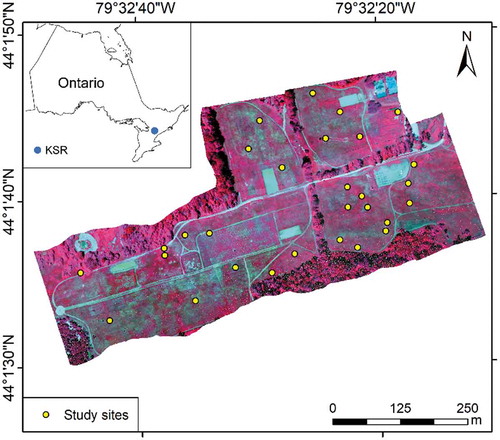
This study was conducted in the Koffler Scientific Reserve (KSR) in Southern Ontario, Canada (Figure 1). It consists of typical temperate tall grasses and is inherently heterogeneous in terms of species composition and growth conditions. Dominant species in this area are Awnless brome (Bromus inermis), Goldenrod (Solidago canadensis L.), Milkweed (Asclepias L.), and Fescue (Festuca rubra L.). The climate type in this area is temperate continental with temperatures ranging from −10°C (February) to 30°C (July) and annual total precipitation from 860 to 1020 mm (Environment Canada 2016). The growing season in this area is from May to September. Trees and forbs are also widely distributed in this area. KSR is a protected area and thus experiences little human disturbance.

Figure 1. Study area (Background is hyperspectral imagery collected on 14 June 2016. RGB composition with bands at 800, 650, and 550 nm. Grasslands are surrounded by treelines, as shown in the figure. Yellow dots represent study sites with 2 × 2 m each in size.)

Leaf sample collection and measurements

Leaf samples were collected, aiming for evaluating the performance of PROSPECT-5, PROSPECT-D, and PROSPECT-5M model. A total of 890 leaf samples at various growth stages (e.g., photosynthetic, senescent, and decay) were collected monthly at KSR in the summer and fall seasons from 2013 to 2016. Leaf samples of 1 ~ 2 dominant species (e.g., Awnless brome, Goldenrod) were collected at each study site. The leaf samples were stored in coolers and were transported back to a wet lab within an hour for spectral and chemical measurements. The spectra of these leaf samples were measured using an ASD FieldSpec spectroradiometer with a Li-Cor 1800 Integrating Sphere (LI-COR Environmental, Lincoln, USA) and a plant probe (Analytical Spectral Devices, Inc. Boulder, USA). The data acquired by the integrating sphere was used for the modeling, and that acquired by the plant probe was used for reference. If a leaf sample was not wide enough to cover the port of the sensor, a leaf mat was made by stitching two or three leaf samples side by side while minimizing overlap. Five spectral measurements were repeated for each sample, and the averaged values were calculated and used as the final leaf spectra. The spectral measurements were performed in a timely manner, trying to minimize the deterioration of leaf samples. After the spectral measurement, chlorophyll contents of leaf samples were extracted using N, N-dimethylformamide (DMF) following the protocol proposed by Minocha et al. (2009). Different parts of the same leaf were used for spectral and chlorophyll measurements, aimed to minimize the potential influence of spectral measurement on the leaf chlorophyll content. Decay pigments (e.g., humic acids) in non-photosynthetic leaf samples were extracted using NaOH as described in Proctor, Lu, and He (2017). Statistics of measured contents of leaf chlorophyll and decay pigments are shown in Table 1.

Table 1. Statistics of measured leaf chlorophyll content, decay pigment content, and canopy LAI

	Minimum	Maximum	Mean
Chlorophyll (µg/cm^2)	0.1	51.8	26.1
Decay pigments (µg/cm^2)	0.01	3.50	2.03
LAI	0.66	4.97	2.35

Hyperspectral imagery collection and field survey

The imaging sensor used in this study was a Micro-HyperSpec, manufactured by Headwall Photonics Inc. (Boston, MA, USA). The sensor was operated in the mode of 325 bands in the range of 400–1000 nm, with 12-bit radiometric resolution, 1.85 nm sampling interval, and 5 nm full width at half maximum (FWHM). This sensor is a push-broom sensor with a CCD matrix of 1004 columns (i.e., pixels) across the spatial dimension and 325 rows across the spectral dimension. With the motion of the platform, the sensor scans an area to acquire an image. A GPS and inertial measuring unit (IMU) were integrated with the sensor to record the locational and orientation information of the sensor. An onboard processing unit was installed for controlling the sensor and storage of imagery. Considering the weight of the imaging system (~2 kg) and the size of the study area, a manned helicopter was used in this study as the flight platform. The helicopter was flown at an average height of 250 m above the ground and 15 m/s speed. The flight height and speed, which control the pixel size in the across-track and along-track directions, respectively, were coordinated to avoid imagery distortion. With an 8-mm focal length that has a field of view (FOV) of 53.2º and an instantaneous FOV of 0.053º, the sensor has a swath of 250 m and acquires imagery with a spatial resolution of 30 cm.

Two flights were performed on 14 June (featured by green canopies with photosynthetic vegetation) and 26 August 2016 (featured by mixed canopies with photosynthetic and non-photosynthetic vegetation). Both flights were carried out at noon with sunny and clear conditions, and each flight took about half an hour. Hyperspectral imagery acquired was radiometrically and geometrically corrected in SpectralView (Headwall Photonics Inc., Boston, MA, USA). Black and white references needed for the radiometric correction were collected by covering the lens with a cap and putting a calibrated standard white reference panel in the field of view, respectively. These references, together with sensor calibration coefficients that were provided by the sensor manufacturer, were then utilized for radiometric correction to convert digital numbers (DNs) to radiance (mW/(cm²× sr×um)). Geometric correction (including orthorectification) of the imagery was performed using GPS data and sensor orientation data acquired by the IMU.

Atmospheric correction of the acquired imagery was conducted using the empirical line method in ENVI to remove the effects of the atmosphere and to convert radiance to reflectance. It is a standard imagery calibration method, removing influences of atmospheric gases and aerosols and converting imagery radiance to reflectance (Lucieer et al. 2014). Two white and two black reference panels were deployed on the ground with 2 m distances between each other. Spectral data of these reference panels were collected using the ASD spectroradiometer as an input for the empirical line method. The ASD data and the hyperspectral imagery were resampled to 2 nm spectral resolution in ENVI for further spectral analysis.

Field surveys were conducted simultaneously with the flights. A total of 34 study sites were pre-selected in the grassland area to cover different terrains, vegetation growing conditions, and species composition (Figure 1). Each site formed a square of 2 m × 2 m on the ground and was differentiated from its surrounding area using colored flagging tapes. Unified white-color foam board labeled with the site ID was fixed on the ground close to each study site, aiming to be visible in the imagery. Locational information for study sites was obtained using highly accurate (e.g., centimeter level) Trimble GeoExplorer GPS (Trimble Navigation Limited, Sunnyvale, CA, USA). Field data collected at the study sites included canopy reflectance, LAI, vegetation height, soil moisture, leaf samples, species composition, and canopy photos. Canopy reflectance data were collected around noontime under clear and sunny weather conditions using an ASD FieldSpec 3 Max field-portable spectroradiometer with a spectral range of 350–2500 nm (Analytical Spectral Devices Inc., Boulder, Colorado, USA). Radiometric calibration of the ASD sensor was conducted every ten minutes using a standard white reference panel that was provided by the sensor manufacturer. Four spectral measurements were performed at 1 m above the ground by holding the sensor at each of four quarter sections of each study site (i.e., a 2 m × 2 m square) to capture potential variations of vegetation, and an averaged reflectance was calculated afterward as the canopy reflectance. The ground-measured canopy reflectance was compared with that extracted from hyperspectral imagery for evaluating the spectral quality of the imagery. LAI was measured using an AccuPAR LP-80 ceptometer (Decagon Devices, Inc., Pullman, Washington, USA). The LAI measurements were also repeated four times at different quarter sections of each study site aimed to acquire average values (Lu and He 2019). Statistics of measured LAI are shown in Table 1. The AccuPAR was calibrated after each measurement. Soil moisture was measured at each of the four quarter sections using HydroSense II (Campbell Scientific, Inc., Logan, Utah, USA), and the averaged value was calculated for each site. Leaf samples were collected randomly from each quarter section, and the leaf spectra and chlorophyll contents were also measured, as described in previous sections. These measured spectral data and vegetation parameters were used for evaluating the performances of different models.

Evaluation of PROSPECT models

The original codes of PROSPECT models were available from http://teledetection.ipgp.jussieu.fr/prosail and were operated in Matlab. In PROSPECT-5, six parameters were used to describe the physical structure and chemical components of leaves (Table 2). In PROSPECT-D, there was one additional parameter, anthocyanins. In the PROSPECT-5M, there were two new pigments, initial decay pigments, and advanced decay pigments, with initial decay pigments replacing the brown pigments in the PROSPECT-5 since their absorption features were similar.

Table 2. Leaf properties considered in different versions of the PROSPECT model

	PROSPECT-5 (Feret et al. 2008)	PROSPECT-D (Feret et al. 2017)	PROSPECT-5M (Proctor, Lu, and He 2017)
Leaf structure	Number of leaf layers	Number of leaf layers	Number of leaf layers
Leaf components	Chlorophyll Carotenoids Brown pigments Water Dry matter	Chlorophyll Carotenoids Brown pigments Water Dry matter Anthocyanins	Chlorophyll Carotenoids Initial decay pigments Advanced decay pigments Water Dry matter

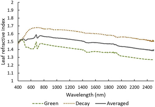
An important parameter in the PROSPECT models is the leaf refractive index, an optical leaf property that controls the light transmission at the air to cell interface. Feret et al. (2008) calculated a refractive index utilizing green leaf samples (hereafter named green refractive index), and Proctor, Lu, and He (2017) estimated a refractive index from decayed leaf samples (hereafter named decay refractive index), which tend to be higher due to the drying of the leaf cells (Figure 2). In this study of mixed canopies, both photosynthetic and non-photosynthetic leaves are present; therefore, an averaged refractive index was used in the PROSPECT-5M model (Figure 2).

Figure 2. Leaf refractive indices for different types of leaves: green (Feret et al. 2008), senescent and decayed (Proctor, Lu, and He 2017), and an averaged version used in this study

PROSPECT-5, PROSPECT-D, and PROSPECT-5M models were then utilized for simulating spectra in the range of 400–2500 nm and estimating chlorophyll contents of the field-collected 890 leaf samples. Parameters used in the models and corresponding value ranges are shown in Table 3. The iterative methods for optimization method (i.e., the fminsearch function in Matlab) was used for inverting the PROSPECT models to identify the best simulated spectra (i.e., lowest RMSE values) from each model (Meienberger 2004; Botha et al. 2010; Jacquemoud and Ustin 2019). The performance of the models for simulating leaf reflectance indicates the model’s effectiveness and reveals spectral ranges that cannot be accurately simulated, which will bring valuable insights for future model improvements.

Table 3. Parameters in the PROSPECT and SAIL models. The value ranges for different parameters are selected based on prior knowledge from field measurements or from literature (Verhoef and Bach 2007; Feret et al. 2008; Jacquemoud et al. 2009; Darvishzadeh et al. 2011; Mousivand et al. 2014; Feret et al. 2017; Proctor, Lu, and He 2017)

Model	Symbol	Quantity	Value range	Unit
PROSPECT	N	Leaf structure parameter	1 ~ 5	-
	Cab	Chlorophyll a + b content	0 ~ 100	µg/cm^2
	Cca	Carotenoids content	0 ~ 30	µg/cm^2
	Cbw	Brown pigments (only used in original PROSPECT-5)	0 ~ 4	-
	Cini	Initial decay pigments content (only used in PROSPECT-5M)	0 ~ 3	µg/cm^2
	Cadv	Advanced decay pigments content (only used in PROSPECT-5M)	0 ~ 1.25	µg/cm^2
	Can	Anthocyanins (only used in PROSPECT-D)	0 ~ 40	µg/cm^2
	Cw	Equivalent water thickness	0 ~ 0.05	cm
	Cm	Dry matter content	0.001 ~ 0.05	g/cm^2
SAIL	LAI	Leaf area index	0 ~ 7	m^2/m^2
	LIDFa	Average leaf angle	20 ~ 40	Deg
	LIDFb	Leaf distribution’s bimodality	0	-
	TypeLIDF	LIDF type	2	-
	tts	Solar zenith angle	22 or 45	Deg
	tto	View zenith angle	0 ~ 30	Deg
	psi	Relative azimuth angle	0 ~ 180	Deg
	hspot	Hot spot parameter	0.01	m/m

Evaluation of PROSAIL using hyperspectral imagery

The PROSPECT models were integrated with a standard SAIL model to create PROSAIL models. PROSAIL models were then tested to simulate reflectance of different types of canopies (e.g., green canopies with photosynthetic vegetation and mixed canopies with photosynthetic and non-photosynthetic vegetation) and to estimate corresponding canopy-level vegetation properties (e.g., LAI and canopy chlorophyll content). Hyperspectral imagery acquired on 14 June and 26 August 2016, representing green and mixed canopies, respectively, were utilized for extracting canopy reflectance data. PROSAIL models were inverted with the imagery reflectance values in the range of 400–1000 nm using a lookup table (LUT) approach to estimate the vegetation properties, such as leaf-level chlorophyll content, water content, and canopy-level LAI. This approach simulates reflectance using all possible parameter value combinations, and performs a global search of LUT to identify the simulated reflectance with the lowest RMSE (i.e., compared with the measured reflectance on a wavelength-by-wavelength basis) and corresponding parameter combination (Darvishzadeh, Matkan, and Ahangar 2012). The parameters and corresponding value ranges for building LUT are shown in Table 3. The parameter combinations corresponding to the best ten simulated reflectance values were examined to determine if they were realistic. For instance, a parameter combination representing a canopy with super high leaf chlorophyll content but super low leaf carotenoid content or super low LAI would not be realistic. The parameter combinations were then averaged as the final estimated vegetation properties (e.g., leaf chlorophyll and water, LAI) (Darvishzadeh et al. 2011). The canopy-level chlorophyll content was then calculated using leaf chlorophyll content times LAI (Darvishzadeh et al. 2010; Wong and He 2013). These estimated values were compared to field-measured values to evaluate the performance of the PROSAIL models.

Description of PROSPECT and SAIL model parameters are shown in Table 3. For the parameters in the SAIL model, LAI, leaf angle, and hot spot parameters were measured in the field. The leaf angles were measured with a digital angle finder. Ten leaves of dominant species were measured to acquire the range and average of the angle values. The hot spot parameter was estimated by leaf length divided by the canopy height (Jarocińska 2014). Solar and view angles were estimated based on the date of imaging and sensor field of view, respectively. Background reflectance (e.g., soil) is a critical variable in PROSAIL and highly influences canopy reflectance, especially for canopies with sparse vegetation. The soil in grasslands is commonly covered by a thick layer of dead materials (e.g., litter). As a result, photons cannot reach the soil, and the degree contribution of soil reflection in the measured reflectance to the total canopy signal is limited. Therefore, an averaged reflectance of the litter layer that was calculated using 35 reflectance values collected at different locations during the field surveys in June and August was applied in the PROSAIL model as the background reflectance (Berger et al. 2018a). These parameters were kept constant between the PROSAIL models.

Results

Results of PROSPECT models

RMSE between the simulated and measured reflectance of photosynthetic and non-photosynthetic leaves with the PROSPECT-5, PROSPECT-D, and PROSPECT-5M model is shown in Figure 3. It can be found that the simulation performance of the PROSPECT-5 and PROSPECT-D was very similar (Figure 3a and b). Specifically, they performed well for photosynthetic leaves, with an average RMSE around 0.01 and a maximum below 0.02. However, for non-photosynthetic leaves, these two models achieved lower accuracy, generating average RMSE around 0.025 and maximum values over 0.05. In terms of the PROSPECT-5M model, it performed similarly well to the PROSPECT-5 and PROSPECT-D for photosynthetic leaves (Figure 3a), while it had a bit higher accuracy over these two models for non-photosynthetic leaves (e.g., average RMSE reduced ~40% to around 0.015 and maximum reduced ~50% to below 0.03, Figure 3b).

Figure 3. Root Mean Square Error (RMSE) of simulated leaf spectra for photosynthetic (Figure a) and non-photosynthetic leaves (Figure b) with the PROSPECT-5, PROSPECT-D, and PROSPECT-5M

To further understand factors influencing the performance of different models and identify spectral ranges that were not well simulated, measured and simulated reflectance of five leaf samples (i.e., photosynthetic or non-photosynthetic leaves of Awnless brome) were compared (Figure 4). The PROSPECT-5 model worked well for simulating reflectance of photosynthetic leaves (e.g., RMSE around 0.010, Figure 4A2 and B2); however, not so for non-photosynthetic leaves (e.g., RMSE generally higher than 0.02, Figure 4C2-E2). For yellow or brown colored leaves with degrading chlorophyll (Figure 4B1 and C1), the model did not properly simulate reflectance in the spectral range of green-red (around 600 nm) and near-infrared (NIR) plateau (approximate 750–1350 nm) with absolute differences reaching 0.06 (i.e., the absolute differences between simulated and measured curves, Figure 4B3 and C3). The PROSPECT-5 simulated the reflectance generally well in the mid-infrared (MIR, approximate 1500–2500 nm) range, with an absolute difference less than 0.04 (Figure 4B3 and C3). For decayed leaves, e.g., gray colored, no chlorophyll, dry, and decomposing leaves (Figure 4D1 and E1), the reflectance was not well simulated in the range of NIR plateau (with absolute differences reaching 0.08) and MIR (with absolute differences around 0.06) (Figure 4B3 and C3). PROSPECT-D performed similarly to PROSPECT-5 for simulating reflectance of the leaf samples: it performed well for photosynthetic leaves (e.g., RMSE around 0.01, Figure 4A2 and B2), but less accurately for non-photosynthetic leaves (e.g., RMSE range from 0.02 to 0.04, Figure 4C2-E2).

Figure 4. Simulation results of photosynthetic and non-photosynthetic leaves using PROSPECT-5, PROSPECT-D, and PROSPECT-5M (second column) and differences between simulated and measured spectra (third column)

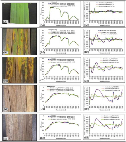
The PROSPECT-5M model had similar performance to the PROSPECT-5 and PROSPECT-D model for photosynthetic leaves, yet achieved higher accuracy for simulating reflectance of non-photosynthetic leaves (Figure 4). Specifically, for green leaves and slightly senescent leaves (Figure 4A1 and B1), the RMSE values of simulations using the PROSPECT-5M model (0.008 and 0.011, respectively) are close to those of simulations using the PROSPECT-5 model (0.010 and 0.013, respectively) or the PROSPECT-D model (0.010 and 0.012, respectively) (Figure 4A2 and B2). In contrast, for deeply senescent leaves and decayed leaves (Figure 4C1, D1, and E1), the RMSE values of simulations using the PROSPECT-5M model (0.015, 0.012, and 0.014, respectively) are reduced from those of simulations using the PROSPECT-5 model (0.023, 0.031, and 0.040, respectively) or the PROSPECT-D model (0.023, 0.031, and 0.041), respectively (Figure 4C2, D2, and E2). Notably, the absolute differences around 600, 900, and 1800 nm of simulated spectra from the PROSPECT-5M model are clearly lower than that from the PROSPECT-5 and PROSPECT-D model (Figure 4C3, D3, and E3). For instance, the absolute differences around 900 nm decrease from around 0.08 to around or below 0.02 (Figure 4C3, D3, and E3). Although the PROSPECT-5M performed better than the other two models, it still did not simulate the reflectance well in a few spectral ranges, including around 450 and 550 nm with absolute differences over 0.02.

Leaf chlorophyll contents estimated using the PROSPECT-5, PROSPECT-D, and PROSPECT-5M models were compared to the measured values to evaluate the performance of these three models, and results are shown in Figure 5. PROSPECT-5, and PROSPECT-D achieved similarly high accuracy for estimating leaf chlorophyll with R² around 0.62 and RMSE around 8.2 µg/cm². The PROSPECT-5M performed slightly better with R² of 0.71 and RMSE of 7.8 µg/cm².

Figure 5. Scatter plots of estimated chlorophyll contents versus measured values using the PROSPECT-5 (a), PROSPECT-D (b), and PROSPECT-5M models (c)

Results of PROSAIL models

The original PROSPECT-5 and PROSPECT-5M were integrated with the canopy-level SAIL model to generate PROSAIL models, and hereafter named original PROSAIL and modified PROSAIL, respectively. PROSPECT-D and PROSPECT-5 model performed very similarly for simulating leaf properties. Therefore, only PROSPECT-5 was selected here for generating a PROSAIL. Performances of the original and modified PROSAIL were compared using data of field sites collected on 14 June (featured by green canopies) and 26 August 2016 (featured by mixed canopies). Accuracy values of the original and modified PROSAIL models for simulating canopy reflectance (i.e., RMSE) are shown in Figure 6. The original and modified PROSAIL performed well for simulating reflectance of green canopies with a mean RMSE around 0.015 and a maximum RMSE slightly over 0.02 (Figure 6a). In contrast, the original and modified PROSAIL models have different performance for simulating reflectance of mixed canopies (Figure 6b). The original PROSAIL has RMSE values ranging from 0.01 to 0.08 and a mean of around 0.035. The modified PROSAIL has higher accuracy, with RMSE reduced ~25% and has a range from 0.01 to 0.05 and a mean of around 0.025 (Figure 6b).

Figure 6. Comparison of original and modified PROSAIL for simulating canopy reflectance with data acquired on (a) 14 June and (b) 26 August 2016

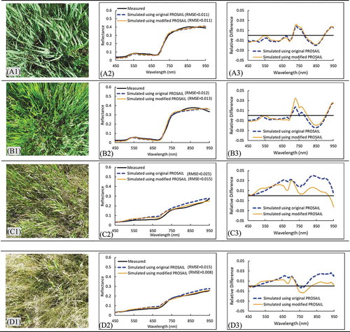
To further understand the performance of original and modified PROSAIL for simulating canopy reflectance along the wavelength, two green and two mixed canopies together with the measured and simulated reflectance were investigated (Figure 7). The original and modified PROSAIL models performed similarly well for simulating reflectance of green canopies (Figure 7A1 and B1; simulation results are shown in Figure 7A2 and B2, RMSE around 0.012). The simulated canopy reflectance curves match well with the measured values along the wavelength from 450 to 950 nm with slight overestimation around 750 nm and underestimation around 850 nm (Figure 7A3 and B3). However, for mixed canopies with a large amount of non-photosynthetic leaves (Figure 7C1 and D1), the original PROSAIL model performed less satisfactorily for simulating canopy reflectance, with RMSE of 0.025 and 0.015 shown in Figure 7C2 and D2, respectively. In contrast, the modified PROSAIL achieved higher accuracies, with RMSE reduced from 0.025 to 0.015 and from 0.015 to 0.008, respectively (Figure 7C2 and D2). Comparing simulated and measured reflectance along the wavelength, it can be found the simulated curve from the original PROSAIL reached higher values than the measured around 650 and 850 nm with absolute differences around 0.03. The modified PROSAIL achieved lower absolute differences around 0.02 (Figure 7C3 and D3).

Figure 7. Simulation results of green (Figure A1 and B1) and mixed canopies (Figure C1 and D1) using original and modified PROSAIL (second column) and differences between simulated and measured curves (third column)

To compare the model’s performances when estimating vegetation properties (e.g., canopy LAI and chlorophyll), the two PROSAIL models were firstly inverted using the image acquired on 14 June 2016, which represented solely green canopies (e.g., as shown in Figure 7A1 and B1). The original PROSAIL performed well for estimating LAI (R² = 0.69, RMSE = 1.03) and canopy chlorophyll content (R² = 0.79, RMSE = 28.3 µg/cm²) (Figure 8a and b). Similarly, the modified PROSAIL model had high accuracy values when estimating LAI (R² = 0.68, RMSE = 0.60) and canopy chlorophyll content (R² = 0.77, RMSE = 25.4 µg/cm²) (Figure 8c and d). It can also be found that both the PROSAIL models slightly overestimated the canopy chlorophyll, especially when the canopy chlorophyll contents are higher than 80 µg/cm² (Figure 8b and d).

Figure 8. Scatter plots of estimated LAI and canopy chlorophyll content versus measured values using the original and modified PROSAIL models for green and mixed canopies (figures a and b correspond to the original model; c and d correspond to the modified model; green color points represent green canopies; brown color points represent mixed canopies)

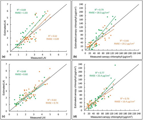
The original and modified PROSAIL models were then inverted to estimate properties of mixed canopies using the imagery acquired on 26 August 2016 (i.e., late growing season). The modified model achieved an accuracy of R² = 0.63 and RMSE = 0.74 for estimating LAI, and R² = 0.76 and RMSE = 16.4 µg/cm² for chlorophyll (Figure 8c and d), which is higher than the accuracy of original model with R² = 0.62 and RMSE = 0.89 for LAI and with R² = 0.66 and RMSE = 20.2 µg/cm² for chlorophyll (Figure 8a and b). The original PROSAIL achieved lower accuracy for mixed canopies than for the green canopies (e.g., estimating LAI with R² decreased from 0.69 to 0.62 and chlorophyll with R² decreased from 0.79 to 0.66, Figure 8a and b). In contrast, the modified PROSAIL model performed similarly well for green and mixed canopies (e.g., estimated LAI with R² around 0.66, estimated chlorophyll with R² around 0.77, Figure 8c and d).

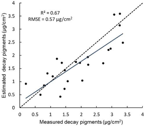
Decay pigments were added in the modified PROSAIL model as parameters (i.e., initial and advanced decay pigment). Thus, the contents of these pigments can also be retrieved through model inversion. Here the decay pigment content is the sum of initial and advanced decay pigment content. As non-photosynthetic vegetation only occurs at late growing stages, only the imagery acquired in August 2016 was utilized for the estimation of decay pigments. A comparison of the model estimated canopy-level decay pigments content and lab measured values is shown in Figure 9. The modified PROSAIL performed well for estimating decay pigments, with R² of 0.67 and RMSE of 0.57 µg/cm².

Figure 9. Comparing PROSAIL estimated canopy-level decay pigment content versus lab measured values

Discussion

The PROSPECT-5 and PROSPECT-D performed well for simulating spectra of photosynthetic leaves (e.g., with mean RMSE below 0.01), which has also been confirmed by previous studies (Feret et al. 2008; Jacquemoud et al. 2009; Feret et al. 2017). However, these two models achieved lower accuracies for simulating spectra of non-photosynthetic leaves (e.g., with mean RMSE around 0.025), which probably because such leaves have different biophysical structures (e.g., leaf thickness) and biochemical components than photosynthetic leaves, which are not fully represented in the models. In terms of biophysical structure, the non-photosynthetic leaves likely have a more disorganized cell structure due to heterogeneous decay and higher refractive index because of drying and decay than that of photosynthetic leaves (Figure 2). For biochemical components, the major ones in photosynthetic and non-photosynthetic leaves, which are listed in Table 4, are also different.

Table 4. Dominant leaf biochemical components of different types of leaves

Leaf biochemical components	Photosynthetic leaves	Non-photosynthetic leaves
Pigments	Chlorophyll, carotenoids, brown pigments	Decay pigments (e.g., humic acid and fulvic acid)
Water	Water (high content)	Water (low content)
Dry matter	Cellulose, hemicellulose, lignin, starch, protein, etc.	Cellulose, hemicellulose, lignin, etc. (decomposed)

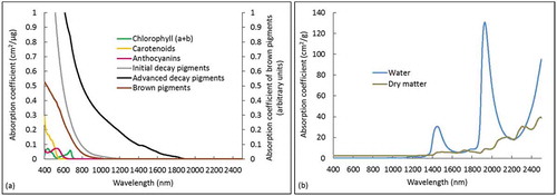
In photosynthetic leaves, chlorophyll and carotenoids are the major pigments, influencing leaf spectra in the visible range (Figure 10a). Brown pigments are not tied to any specific biochemicals, and assumed to be tannins (Jacquemoud and Baret 1990) or polyphenols (Baret and Fourty 1997). The brown pigments are distinguished from photosynthetic pigments as having a longer absorption curve (up to 1300 nm) (Figure 10a). The dry matter in PROSPECT-5 is a composition of various chemicals, such as cellulose and lignin, which absorb radiation in the shortwave infrared (Figure 10b). Its influence is masked in photosynthetic vegetation by the much stronger absorption of water in a similar wavelength range (Fourty et al. 1996). When leaf senescence starts, chlorophyll and carotenoids degrade (degradation of carotenoids may be incomplete and thus causing an increasing ratio of carotenoids per chlorophyll), and the leaf water content decreases, and consequently, the absorption features of dry matter appear (Junker and Ensminger 2016). Meanwhile, leaf constituents (e.g., sugars, amino acids, and cellulose) are decomposed by microbes, and the waste and end-products become decay pigments (e.g., humic and fulvic acids); thus, the leaves will begin to transition into the dark brown and gray colors of decay pigments (Proctor, Lu, and He 2017). Absorption effects of these decay pigments highly influence the leaf spectra in the visible and near-infrared ranges and have further impacts into the middle infrared up to ~1900 nm (Figure 10a). The PROSPECT-5 and PROSPECT-D did not consider such absorption effects and thus cannot accurately simulate the spectra of non-photosynthetic leaves. One clear evidence is that the simulated reflectance curves from these two models are much higher than the measured ones in the range of 750–1200 nm (Figure 4C3 to E3), in which range strong absorptions of decay pigments are observed (Figure 10a). The PROSPECT-5M model considered the absorption effects of these decay pigments, and thus it performed better than the PROSPECT-5 and PROSPECT-D model. This also confirms the possibility of using RTMs for quantifying biochemical components of non-photosynthetic vegetation, which is critical for evaluating vegetation senescent and decay status and understanding plant-soil nutrition cycles. However, the decay pigments is a term describing a combination of different pigments that are produced during senescent and decay processes, including humic acid and fulvic acid. It is suggested to specify these pigments in future model developments (e.g., retrieve specific absorption coefficients of humic and fluvic acids, identify other dominant acids in decay pigments).

Figure 10. Absorption coefficients of leaf chemical components that are considered in different PROSPECT models (Feret et al. 2008, 2017; Proctor, Lu, and He 2017). Specific components considered in each model can be found in Table 2. Absorption coefficients of brown pigments use arbitrary units (i.e., the secondary y-axis in figure a)

The PROSPECT-5M did not simulate the leaf spectra well in a few specific ranges (e.g., absolute difference with the measured reflectance around 0.03). For instance, this model underestimated the reflectance in 400–500 nm for decayed leaves (Figure 4D3 and E3). This is mainly because the decay pigments used in the model have very high absorption coefficients in this range (Figure 10a). Compared with the simulated reflectance from PROSPECT-5 and PROSPECT-D, the involvement of decay pigments in PROSPECT-5M contributed to the accurate simulation in 500–2500 nm, but not in 400–500 nm. Further calibration of absorption coefficients of decay pigments, especially in the 400–500 nm, is needed. In addition, although the PROSPECT-5M performed better than the PROSPECT-5 and PROSPECT-D for simulating reflectance in most spectral ranges, still it overestimated at 700–900 and around 1800 nm and underestimated in 900–1300 nm for early senescent leaves (Figure 4B3 and C3). However, such over- or under-estimations were reduced for decayed leaves (Figure 4D3 and E3). This is because the PROSPECT-5M model was calibrated with mainly decayed leaves from a relatively small number of monocot species. Therefore, the model performance on decay leaves is better than that on early senescent leaves. This reveals how well the PROSPECT-5M and decay pigments work for species and leaf situations not explicitly modeled, which indicates the transferability of the model. It is also important to note that the assumption in PROSPECT-5M is that the absorption properties of decay pigments are the same between all species and for leaves at different physiological stages, and thus likely, they cannot reflect the real leaf situations. Further investigation on the decay pigments in leaves of a wider array of species and at different physiological stages is warranted. In addition, the averaged refractive index used in the PROSPECT-5M may also affect the model performance. It is the average of the green and decay refractive indices, and thus it cannot represent the actual spectral properties of green or decay leaves. An alternative approach is using a dynamic refractive index, and that the green or decay refractive indices can be selected according to the leaf status, which potentially will improve the accuracy of PROSPECT-5M. However, this would complicate the model and could result in inappropriate “tuning” of this parameter during model inversion. Further examination of using different refractive indices is warranted. Besides the model parameters, there were also some uncertainties associated with the leaf spectral measurements that can affect the model performance. For instance, gaps between the leaves when made leaf mats and leaf deterioration during the spectral measurements may influence the quality of spectral data and consequently impact the performance of models. Further exploration of these uncertainties is also warranted.

Involving more pigments as new parameters in RTMs to capture their specific absorption features will likely improve the model performance, which, however, also depends on the application scenario. For instance, adding decay pigments in PROSPECT-5M did not improve the model performance for green leaves, as such leaves contain little decay pigments. Similarly, compared with PROSPECT-5, adding anthocyanins in the PROSPECT-D did not improve its performance for grass leaves, which is because the anthocyanins are not a major pigment in grasses. Model inversion of PROSPECT-D estimated that most grass samples had very low anthocyanins content (less than 3 µg/cm²), much lower than that in the leaves of other species such as Maple tree or Hazel with anthocyanins content of an averaged 8 µg/cm², and as high as 30 µg/cm² (Feret et al. 2017). The PROSPECT-D model also did not perform better than the PROSPECT-5 for non-photosynthetic leaves because the newly added parameter anthocyanins have spectral absorption until 600 nm (Figure 10a). It cannot capture the absorption features of non-photosynthetic leaves from 600–1900 nm. Therefore, it is important to understand leaf properties (e.g., if leaves contain a considerable amount of decay pigments or anthocyanins) when selecting PROSPECT models. It is not ideal to select the model with the most parameters as it may reduce the computing efficiency and cause an ill-posed problem.

At the canopy level, the original and modified PROSAIL models had similar performance for simulating reflectance and estimating properties (e.g., LAI and chlorophyll) of green canopies (Figure 8). This is because they used similar PROSPECT and the same SAIL model. Although new parameters (e.g., decay pigments) were involved in the PROSPECT-5M, they have little contribution to the model simulation for the green canopies since photosynthetic leaves do not have much decay pigments. In contrast, for mixed canopies with photosynthetic and non-photosynthetic vegetation, the modified PROSAIL model performed better than the original version for simulating the canopy reflectance and estimating properties. For instance, the canopy reflectance simulated by the original PROSAIL was consistently higher than the measured, while that simulated by the modified PROSAIL was closer (Figure 7C3 and D3). This is because the PROSPECT-5M model in the modified PROSAIL considered the strong absorption effects of decay pigments in this spectral range and was more capable of simulating spectra of non-photosynthetic vegetation. Therefore, if the research focuses on green canopies, different versions of PROSAIL generally will perform well. However, if the research involves a substantial amount of mixed canopies with photosynthetic and non-photosynthetic vegetation, potential limitations of PROSAIL need to be considered. It was also found that both the original and modified PROSAIL overestimated chlorophyll content for green canopies, while underestimated chlorophyll for mixed canopies (Figure 8c and d). These features correspond to the underestimation of reflectance for green canopies and overestimation for mixed canopies, respectively, in the chlorophyll absorption ranges (i.e., blue and red) by these two modes (Figure 7). Further model calibrations are thus needed to improve the spectral simulation capacity in these ranges and thus to improve the model performance of estimating chlorophyll content. It can also be found in Figure 8 that there are two groups of points with relatively low and high LAI values (or canopy chlorophyll content), respectively, for the estimation of mixed canopies (i.e., brown color points), resulting from different species and their phenological features. One dominant species, Awnless Brome, is senescent in August, and the plants have low LAI and canopy chlorophyll content. However, another dominant species, Goldenrod, is flourishing with dense and green canopies in August, causing points with high LAI and canopy chlorophyll contents in Figure 8. Therefore, species composition and phenological features likely affect the performance of PROSAIL. It is thus worth exploring if differentiating species and separately applying the models will improve the modeling accuracy.

One limitation in this research is with the SAIL model, in which the entire canopy is assumed to have one leaf type; hence it does not represent the mixing ratio and positions of photosynthetic and non-photosynthetic leaves and their distribution within the canopy (Berger et al. 2018a). In mixed scenes, where the canopy is comprised of photosynthetic and non-photosynthetic leaves in various fractions, pooling these leaf types into a single leaf that represents the “average” biochemical contents may not sufficiently represent the course of light-matter interactions that occur. Alternative strategies could be the use of multiple-leaf canopy models, such as the 4SAIL2 model (Verhoef and Bach 2007), in which two types of leaves are accounted for separately. The original PROSPECT model and 4SAIL2 model were integrated with the soil-leaf-canopy (SLC) model (Verhoef and Bach 2007), which potentially can better simulate spectra of mixed canopies.

Conclusions

This study investigated three PROSPECT models (i.e., PROSPECT-5, PROSPECT-D, and PROSPECT-5M) for understanding their performance and limitation at simulating the spectra of photosynthetic and non-photosynthetic leaves. The three models achieved similar accuracies for simulating spectra of photosynthetic leaves. However, the PROSPECT-5M performed better than the other two models for non-photosynthetic leaves, owning to the involvement of decay pigments that have considerable absorption effects in the visible to shortwave infrared ranges. The PROSPECT-5 and PROSPECT-5M were integrated with the SAIL model to generate an original and a modified PROSAIL, respectively, for simulating vegetation properties of different types of canopies (e.g., green or mixed). The two PROSAIL models had a similar performance for green canopies, while the modified PROSAIL achieved higher accuracy than the original version for mixed canopies. The better performance of the PROSPECT-5M model on non-photosynthetic leaves contributed to the higher simulation accuracy of modified PROSAIL on mixed canopies.

Adding decay pigments as parameters in the PROSPECT-5M and modified PROSAIL extended the applicability of these models from simulating properties of photosynthetic vegetation to both photosynthetic and non-photosynthetic vegetation. However, unique decomposition pathways producing unique pigments and spectra are likely to occur in nature. Although this research has shown promising results in the application of the PROSPECT-5M and modified PROSAIL models to vegetation types outside of the calibration range (e.g., species and leaves at different physiological stages), further work is needed on model validation and whether two decay pigments are sufficient to simulate the spectral behavior of non-photosynthetic vegetation across the world’s ecosystems and environmental conditions.

Lastly, RTM is expected to be a robust and transferable approach for simulating vegetation spectra and estimating vegetation properties at different levels (e.g., leaf level and canopy level). Popular RTMs, such as PROSPECT and PROSAIL, have been successfully applied in many previous studies. However, each ecosystem (e.g., forests, crops, grasslands, or wetlands) has its own vegetation biophysical and biochemical properties, such as leaf structure, leaf biochemical components (e.g., having decay pigments or anthocyanins), canopy structure, and soil background. Therefore, when applying RTMs for simulation, careful model selection, evaluation, and potential modifications are essential for success.

Acknowledgements

This study was funded by the Natural Sciences and Engineering Research Council of Canada (NSERC) Discovery Grant [RGPIN-386183] to Dr. Yuhong He; the New Faculty Start-Up Grant to Dr. Bing Lu at the Simon Fraser University; and the Graduate Expansion Funds to Dr. Bing Lu in the Department of Geography, University of Toronto Mississauga. Thanks to the managers of the Koffler Scientific Reserve and to a group of research field assistants at the University of Toronto Mississauga who helped with fieldwork.

Disclosure statement

No potential conflict of interest was reported by the authors.

Data availability statement

Parameters in the PROSPECT-5M model, including specific absorption coefficients of initial and advanced decay pigments and decay refractive index, are available from the following repository https://github.com/drproctorWindsor/DecompositionPigments.

Additional information

Funding

This work was supported by the Natural Sciences and Engineering Research Council of Canada [RGPIN-386183]; University of Toronto Mississauga-Geography [Graduate Expansion Funds]; Simon Fraser University [New Faculty Start-Up Grant].

References

- Atzberger, C., R. Darvishzadeh, M. Immitzer, M. Schlerf, A. Skidmore, and G. le Maire. 2015. “Comparative Analysis of Different Retrieval Methods for Mapping Grassland Leaf Area Index Using Airborne Imaging Spectroscopy.” International Journal of Applied Earth Observation and Geoinformation 43: 19–31. doi:10.1016/j.jag.2015.01.009.
- Atzberger, C., R. Darvishzadeh, M. Schlerf, and G. Le Maire. 2013. “Suitability and Adaptation of PROSAIL Radiative Transfer Model for Hyperspectral Grassland Studies.” Remote Sensing Letters 4 (1): 56–65. doi:10.1080/2150704X.2012.689115.
- Baret, F., and T. Fourty. 1997. “Estimation of Leaf Water Content and Specific Leaf Weight from Reflectance and Transmittance Measurements.” Agronomie 17 (9–10): 455–464. doi:10.1051/agro:19970903.
- Berger, K., C. Atzberger, M. Danner, G. D’Urso, W. Mauser, F. Vuolo, and T. Hank. 2018a. “Evaluation of the PROSAIL Model Capabilities for Future Hyperspectral Model Environments: A Review Study.” Remote Sensing 10 (851). doi:10.3390/rs10010085.
- Berger, K., C. Atzberger, M. Danner, G. D. Urso, W. Mauser, F. Vuolo, and T. Hank. 2018b. “Evaluation of the PROSAIL Model Capabilities for Future Hyperspectral Model Environments: A Review Study.” Remote Sensing 10 (2): 85. doi:10.3390/rs10010085.
- Berger, K., C. Atzberger, M. Danner, M. Wocher, W. Mauser, and T. Hank. 2018c. “Model-Based Optimization of Spectral Sampling for the Retrieval of Crop Variables with the PROSAIL Model.” Remote Sensing 10 (12): 2063. doi:10.3390/rs10122063.
- Botha, E. J., B. Leblon, B. J. Zebarth, and J. Watmough. 2010. “Non-Destructive Estimation of Wheat Leaf Chlorophyll Content from Hyperspectral Measurements through Analytical Model Inversion.” International Journal of Remote Sensing 31 (7): 1679–1697. doi:10.1080/01431160902926574.
- Bousquet, L., S. Lacherade, S. Jacquemoud, and I. Moya. 2005. “Leaf BRDF Measurements and Model for Specular and Diffuse Components Differentiation.” Remote Sensing of Environment 98 (2–3): 201–211. doi:10.1016/j.rse.2005.07.005.
- Colombo, R. 2003. “Retrieval of Leaf Area Index in Different Vegetation Types Using High Resolution Satellite Data.” Remote Sensing of Environment 86 (1): 120–131. doi:10.1016/S0034-4257(03)00094-4.
- Danson, F. M., C. S. Rowland, and F. Baret. 2003. “Training a Neural Network with a Canopy Reflectance Model to Estimate Crop Leaf Area Index.” International Journal of Remote Sensing 24 (23): 4891–4905. doi:10.1080/0143116031000070319.
- Darvishzadeh, R., C. Atzberger, A. Skidmore, and M. Schlerf. 2010. “Retrieval of Vegetation Biochemicals Using a Radiative Transfer Model and Hyperspectral Data.” 100 Years ISPRS Advancing Remote Sensing Science, PT 2 38 (7B): 171–175.
- Darvishzadeh, R., C. Atzberger, A. Skidmore, and M. Schlerf. 2011. “Mapping Grassland Leaf Area Index with Airborne Hyperspectral Imagery: A Comparison Study of Statistical Approaches and Inversion of Radiative Transfer Models.” Isprs Journal of Photogrammetry and Remote Sensing 66 (6): 894–906. doi:10.1016/j.isprsjprs.2011.09.013.
- Darvishzadeh, R., A. A. Matkan, and A. D. Ahangar. 2012. “Inversion of a Radiative Transfer Model for Estimation of Rice Canopy Chlorophyll Content Using a Lookup-Table Approach.” IEEE Journal of Selected Topics in Applied Earth Observations and Remote Sensing 5 (4SI): 1222–1230. doi:10.1109/JSTARS.2012.2186118.
- Darvishzadeh, R., A. Skidmore, M. Schlerf, and C. Atzberger. 2008. “Inversion of a Radiative Transfer Model for Estimating Vegetation LAI and Chlorophyll in a Heterogeneous Grassland.” Remote Sensing of Environment 112 (5): 2592–2604. doi:10.1016/j.rse.2007.12.003.
- Duan, S., Z. Li, H. Wu, B. Tang, L. Ma, E. Zhao, and C. Li. 2014. “Inversion of the PROSAIL Model to Estimate Leaf Area Index of Maize, Potato, and Sunflower Fields from Unmanned Aerial Vehicle Hyperspectral Data.” International Journal of Applied Earth Observation and Geoinformation 26: 12–20. doi:10.1016/j.jag.2013.05.007.
- Environment Canada. 2016. “Historical Climate Data.” http://climate.weather.gc.ca/
- Féret, J., K. Berger, F. de Boissieu, and Z. Malenovský. 2021. “PROSPECT-PRO for Estimating Content of Nitrogen-Containing Leaf Proteins and Other Carbon-Based Constituents.” Remote Sensing of Environment 252: 112173. doi:10.1016/j.rse.2020.112173.
- Feret, J., C. Francois, G. P. Asner, A. A. Gitelson, R. E. Martin, L. P. R. Bidel, S. L. Ustin, G. le Maire, and S. Jacquemoud. 2008. “PROSPECT-4 and 5: Advances in the Leaf Optical Properties Model Separating Photosynthetic Pigments.” Remote Sensing of Environment 112 (6): 3030–3043. doi:10.1016/j.rse.2008.02.012.
- Feret, J. B., A. A. Gitelson, S. D. Noble, and S. Jacquemoud. 2017. “PROSPECT D Towards Modeling Leaf Optical Properties through a Complete Lifecycle.” Remote Sensing of Environment 193: 204–215. doi:10.1016/j.rse.2017.03.004.
- Fourty, T., F. Baret, S. Jacquemoud, G. Schmuck, and J. Verdebout. 1996. “Leaf Optical Properties with Explicit Description of Its Biochemical Composition: Direct and Inverse Problems.” Remote Sensing of Environment 56 (2): 104–117. doi:10.1016/0034-4257(95)00234-0.
- Gould., K., K. Davies, and C. Winefield. 2009. Anthocyanins: Biosynthesis, Functions, and Applications.In. New York, NY: Springer-Verlag.
- Guerschman, J. P., M. J. Hill, L. J. Renzullo, D. J. Barrett, A. S. Marks, and E. J. Botha. 2009. “Estimating Fractional Cover of Photosynthetic Vegetation, Non-Photosynthetic Vegetation and Bare Soil in the Australian Tropical Savanna Region Upscaling the EO-1 Hyperion and MODIS Sensors.” Remote Sensing of Environment 113 (5): 928–945. doi:10.1016/j.rse.2009.01.006.
- Jacquemoud, S., C. Bacour, H. Poilve, and J. P. Frangi. 2000. “Comparison of Four Radiative Transfer Models to Simulate Plant Canopies Reflectance: Direct and Inverse Mode.” Remote Sensing of Environment 74 (3): 471–481. doi:10.1016/S0034-4257(00)00139-5.
- Jacquemoud, S., and F. Baret. 1990. “PROSPECT - a Model of Leaf Optical-Properties Spectra.” Remote Sensing of Environment 34 (2): 75–91. doi:10.1016/0034-4257(90)90100-Z.
- Jacquemoud, S., and S. Ustin. 2019. Leaf Optical Properties. Cambridge: Cambridge University Press.
- Jacquemoud, S., S. L. Ustin, J. Verdebout, G. Schmuck, G. Andreoli, and B. Hosgood. 1996. “Estimating Leaf Biochemistry Using the PROSPECT Leaf Optical Properties Model.” Remote Sensing of Environment 56 (3): 194–202. doi:10.1016/0034-4257(95)00238-3.
- Jacquemoud, S., W. Verhoef, F. Baret, C. Bacour, P. J. Zarco-Tejada, G. P. Asner, C. Francois, and S. L. Ustin. 2009. “PROSPECT Plus SAIL Models: A Review of Use for Vegetation Characterization.” Remote Sensing of Environment 113: S56–S66. doi:10.1016/j.rse.2008.01.026.
- Jarocińska, A. M. 2014. “Radiative Transfer Model Parametrization for Simulating the Reflectance of Meadow Vegetation.” Miscellanea Geographica 18 (2): 5–9. doi:10.2478/mgrsd-2014-0001.
- Junker, L. V., and I. Ensminger. 2016. “Relationship between Leaf Optical Properties, Chlorophyll Fluorescence and Pigment Changes in senescingAcer Saccharum Leaves.” Tree Physiology 36 (6): 694–711. doi:10.1093/treephys/tpv148.
- Le Maire, G., C. Francois, and E. Dufrene. 2004. “Towards Universal Broad Leaf Chlorophyll Indices Using PROSPECT Simulated Database and Hyperspectral Reflectance Measurements.” Remote Sensing of Environment 89 (1): 1–28. doi:10.1016/j.rse.2003.09.004.
- Li, Z., and X. Guo. 2018. “Non-Photosynthetic Vegetation Biomass Estimation in Semiarid Canadian Mixed Grasslands Using Ground Hyperspectral Data, Landsat 8 OLI, and Sentinel-2 Images.” International Journal of Remote Sensing 39 (20): 6893–6913. doi:10.1080/01431161.2018.1468105.
- López, R., D. Gondar, A. Iglesias, S. Fiol, J. Antelo, and F. Arce. 2008. “Acid Properties of Fulvic and Humic Acids Isolated from Two Acid Forest Soils under Different Vegetation Cover and Soil Depth.” European Journal of Soil Science 59 (5): 892–899. doi:10.1111/j.1365-2389.2008.01048.x.
- Lu, B., and Y. He. 2019. “Leaf Area Index Estimation in a Heterogeneous Grassland Using Optical, SAR, and DEM Data.” Canadian Journal of Remote Sensing 45 (5): 618–633. doi:10.1080/07038992.2019.1641401.
- Lucieer, A., Z. Malenovský, T. Veness, and L. Wallace. 2014. “HyperUAS-imaging Spectroscopy from a Multirotor Unmanned Aircraft System.” Journal of Field Robotics 31 (4): 571–590. doi:10.1002/rob.21508.
- Meienberger, G. 2004. Canopy Biophysical Parameter Retrieval by Inversion of the PROSPECT-SAIL Radiative Transfer Models Using Three Different Techniques: An Iterative Minimisation Algorithm, a Look-Up Table Approach and a Neural Network, University of Zürich.
- Minocha, R., G. Martinez, B. Lyons, and S. Long. 2009. “Development of a Standardized Methodology for Quantifying Total Chlorophyll and Carotenoids from Foliage of Hardwood and Conifer Tree Species.” Canadian Journal of Forest Research 39 (4): 849–861. doi:10.1139/X09-015.
- Mousivand, A., M. Menenti, B. Gorte, and W. Verhoef. 2014. “Global Sensitivity Analysis of the Spectral Radiance of a Soil–Vegetation System.” Remote Sensing of Environment 145: 131–144. doi:10.1016/j.rse.2014.01.023.
- Pedros, R., Y. Goulas, S. Jacquemoud, J. Louis, and I. Moya. 2010. “FluorMODleaf: A New Leaf Fluorescence Emission Model Based on the PROSPECT Model.” Remote Sensing of Environment 114 (1): 155–167. doi:10.1016/j.rse.2009.08.019.
- Proctor, C., B. Lu, and Y. He. 2017. “Determining the Absorption Coefficients of Decay Pigments in Decomposing Monocots.” Remote Sensing of Environment 199: 137–153. doi:10.1016/j.rse.2017.07.007.
- Rivera, J., J. Verrelst, G. Leonenko, and J. Moreno. 2013. “Multiple Cost Functions and Regularization Options for Improved Retrieval of Leaf Chlorophyll Content and LAI through Inversion of the PROSAIL Model.” Remote Sensing 5 (7): 3280–3304. doi:10.3390/rs5073280.
- Schlerf, M., and C. Atzberger. 2006. “Inversion of a Forest Reflectance Model to Estimate Structural Canopy Variables from Hyperspectral Remote Sensing Data.” Remote Sensing of Environment 100 (3): 281–294. doi:10.1016/j.rse.2005.10.006.
- Verhoef, W., and H. Bach. 2007. “Coupled Soil-Leaf-Canopy and Atmosphere Radiative Transfier Modeling to Simulate Hyperspectral Multi-Angular Surface Reflectance and TOA Radiance Data.” Remote Sensing of Environment 109 (2): 166–182. doi:10.1016/j.rse.2006.12.013.
- Vohland, M., S. Mader, and W. Dorigo. 2010. “Applying Different Inversion Techniques to Retrieve Stand Variables of Summer Barley with PROSPECT+SAIL.” International Journal of Applied Earth Observation and Geoinformation 12 (2): 71–80. doi:10.1016/j.jag.2009.10.005.
- Wong, K. K., and Y. He. 2013. “Estimating Grassland Chlorophyll Content Using Remote Sensing Data at Leaf, Canopy, and Landscape Scales.” Canadian Journal of Remote Sensing 39 (2): 155–166. doi:10.5589/m13-021.
- Yildirim, E. 2007. “Foliar and Soil Fertilization of Humic Acid Affect Productivity and Quality of Tomato.” Acta Agriculturae Scandinavica. Section B, Soil and Plant Science 57 (2): 182–186. doi:10.1080/09064710600813107.
- Zarco-Tejada, P. J., J. R. Miller, J. Harron, B. Hu, T. L. Noland, N. Goel, G. H. Mohammed, and P. Sampson. 2004. “Needle Chlorophyll Content Estimation through Model Inversion Using Hyperspectral Data from Boreal Conifer Forest Canopies.” Remote Sensing of Environment 89 (2): 189–199. doi:10.1016/j.rse.2002.06.002.