The impact of indicator selection on assessment of global greening

ABSTRACT

Greening represents a significant increase in vegetation activity. Accurate quantification of global greening in peak growth is vital for quantifying changes in terrestrial productivity. Normalized Difference Vegetation Index (NDVI) is the remote sensing indicator most commonly applied for this purpose. However, there is limited knowledge about how the applications of other improved or newly available products can impact global greening assessments. This study reports the first systematic investigation of the impact of vegetation indicator selection on global greening in peak growth. It examines the period from 2003 to 2017 using six indicators with a spatial resolution of 500 m: Near Infrared Reflectance of terrestrial vegetation (NIRv) and the coupled diagnostic biophysical modeled Gross Primary Production (PML-GPP), together with NDVI, Enhanced Vegetation Index with two bands (EVI2), Leaf Area Index (LAI) and Moderate Resolution Imaging Spectroradiometer (MODIS) GPP (MOD-GPP) calculated based on MODIS images. Vegetation trends were estimated using the Mann–Kendall test, the unanimous trends by six vegetation indicators were derived, and the concordance ratio in estimated trends by each pair of indicators was investigated among different biomes and their sensitivity to changes in climate were investigated. We found that the estimated greening and browning varied between 12–23% and 2–13% of the vegetated areas, respectively. There was more net greening estimated from NDVI and MOD-GPP (around 19%) compared to the other indicators (8–11%). The concordance ratio between EVI2 and NIRv was much higher (>94%) than other combinations (61–76%) at the global scale. The concordance ratio between one specific indicator and the other indicators gradually increased with its change magnitude. Unanimous results from these six indicators were exhibited in less than two-fifths (38.71%) of vegetated areas. Apart from the EVI2 and NIRv, the concordance ratio varied among different biomes: high in cropland (67–81%), but low in deciduous needle-leaf forest (51–62%) and very low in evergreen broadleaf forest between PML-GPP and others (37–49%). The diverse sensitivity to changes in climate contributed to the discrepancies: greening was more pronounced during warming conditions for the GPP products when compared with the greenness indices. At the global scale, the concordance ratio was higher during cooling conditions among all the indicators except between PML-GPP. Datasets supporing these findings are available online at https://github.com/FuzhouSIRC/Greening_6indicators.2

KEYWORDS:

• Global greening
• vegetation indicators
• gpp
• concordance ratio
• discrepancy

1. Introduction

Vegetation productivity is the basis of all the biosphere functions on the land surface (Schwalm et al. 2017), which provides food, fiber, fuel, and other valuable ecosystem services (Piao et al. 2020). Greening represents a significant increase in vegetation activities and understanding of changes in vegetation productivity are essential issues in global ecology research (De Jong et al. 2012; Murthy and Bagchi 2018; Zhang et al. 2017b). It is impossible to detect spatio-temporal vegetation trends at the global scale using ground-based observations; but, remote-sensed datasets provide the only viable way for this purpose over multi-decadal time periods (Burrell, Evans, and Liu 2018; Piao et al. 2020). Vegetation indices (greenness indices) and Gross Primary Productivity (GPP) products have been widely used for assessing spatio-temporal variability of vegetation productivity as these products can overcome the lack of extensive flux tower observations from large areas (Chen et al. 2019; Myers-Smith et al. 2020; Schwalm et al. 2017; Zhu et al. 2016).

A number of vegetation indices have been developed based on the reflectance data (i.e., in red and near-infrared bands) of remote sensing images (Myneni et al. 1995). Among them, Normalized Difference Vegetation Index (NDVI) is the most widely used vegetation indices for estimating vegetation productivity (Bianchi, Villalba, and Solarte 2020). However, NDVI could be influenced by soil reflectance, and saturates in dense canopies (i.e., NDVI becomes insensitive at high values of leaf area index) (Pettorelli et al. 2005). The Enhanced Vegetation Index with two bands (EVI2) makes improvements and does not saturate in dense canopies (Jiang et al. 2008). Trends in vegetation productivity can also be defined as the significant changes in leaf area index (LAI) (Zhu et al. 2016). Besides the commonly applied radiometric greenness (NDVI, EVI2, LAI), a recently proposed vegetation index, Near Infrared Reflectance of terrestrial vegetation (NIRv), was found to be strongly correlated with tower GPP and accurately predicts photosynthesis without environmental factors (Badgley et al., 2019). However, it is still unclear whether and how vegetation productivity has increased in the last two decades when the NIRv is used for estimation.

Global GPP products have been estimated through a combined consideration of vegetation and environmental conditions using either remote sensing data-driven models or process-based models (Zhang et al. 2019). Remote sensing data-driven models calculate GPP as the product of incident photosynthetically active radiation (PAR), the fraction of absorbed PAR (fAPAR) and light-use efficiency (LUE), where fAPAR is typically assumed to be linearly correlated with vegetation indices and LUE is differentiated by vegetation type (Heinsch et al. 2004). MODIS GPP (MOD-GPP) is one of the widely applied remote sensing driven GPP products, but there are distortions in the spatio-temporal patterns (Zhang et al. 2012). More sophisticated approaches, i.e., process-based models, have been recently developed (Zhang et al. 2019). For example, the coupled diagnostic biophysical modeled GPP (PML-GPP) which uses MODIS data (leaf area index, albedo, and emissivity) together with GLDAS meteorological forcing data as model inputs, which was reported to perform better than most GPP products (Zhang et al. 2019).

Vegetation indices and GPP products are not direct measurements of photosynthesis and contain errors and uncertainties (Burrell, Evans, and Liu 2018). Large discrepancies and uncertainties have been recently revealed in different satellite-derived products of vegetation indices (i.e., NDVI, LAI) (Alcaraz‐Segura et al. 2010; Beck et al. 2011; Jiang et al. 2017; Scheftic et al. 2014). One challenge concerning uncertainties is better incorporating and accounting for different scales of observation and uncertainty in the analyses of changing vegetation productivity (Myers-Smith et al. 2020).Weak agreement between the trends in the datasets highlights the significance of using multiple datasets to evaluate global greening (Scheftic et al. 2014). However, global studies on vegetation changes are generally conducted using remote sensing images with a spatial resolution of 5 km or above (Beck et al. 2011; Chen et al. 2019). Sub-pixel spatial heterogeneity in vegetative greening and browning cannot be accurately captured at coarser grains since spatial heterogeneity in land cover can influence the relationship (Myers-Smith et al. 2020). Despite the well-documented discrepancies between the vegetation indices and GPP products (Yang et al. 2018; Zhao and Running 2010), there is limited knowledge on impacts of indicators selections on the estimated greening when datasets with higher spatial resolution (i.e., 500 m) at the global scale are used.

Annual peak growth of vegetation is critical in characterizing the capacity of terrestrial productivity (Huang et al. 2018; Park et al. 2019). However, despite numerous reporting of a greening earth (Chen et al. 2019; Piao et al. 2020), the enchantment of peak growth globally has not been widely investigated (Huang et al. 2018). This study was conducted to improve our understanding of how vegetation indicator selection would influence the assessment of global greening in peak growth using commonly applied indicators (NDVI, EVI2, LAI, MOD-GPP) as well as new products (NIRv and PML-GPP) with a spatial resolution of 500 m. The following two research hypotheses were proposed in this study: (1) the consistency of estimated trends between each pair of indicators should be greater than 80%, and NDVI was expected to gain higher consistency with other indicators since other vegetation indices were either developed or modified based on the NDVI function; (2) the extent of consistency will vary depending on climatic conditions.

2. Materials and methods

1.1. Data sources

1.1.1. Eight-day composite time series datasets of six vegetation indicators

Eight-day composites of global 500 m time series datasets were developed for these six vegetation indicators: NDVI, EVI2, NIRv, LAI, and two GPP products (MOD-GPP, PML-GPP). Surface spectral reference data for 8-Day Global 500 m MOD09A1.006 Terra Surface Reflectance from 2003 to 2017 were used to calculate NDVI, EVI2, and NIRv (Badgley, Field, and Berry 2017; Jiang et al. 2008). The 4-Day Global 500 m MODIS LAI (MCD15A3H.006) data were aggregated to 8-day composite time series. Two 8-day global 500 m GPP products were the MOD17A2H V6 GPP product (MOD-GPP) (Heinsch et al. 2004) and the PML-GPP (Zhang et al. 2019). The Google Earth Engine (GEE) provides a cloud platform to access and process all these time series datasets (Table S1). The FluxCom GPP (Tramontana et al. 2016) was not considered due to its unavailability from the GEE.

1.1.2. Monthly datasets of climatic variables

Climate data were derived from the Famine early warning systems network Land Data Assimilation System (FLDAS) (McNally et al. 2017). The FLDAS is a custom instance of the NASA Land Information System. This dataset contains a series of land surface parameters including global monthly air temperature and precipitation with a spatial resolution of 0.1° (Table S1).

1.1.3. Land cover dataset

The MODIS yearly land cover product (MCD12Q1) with a spatial resolution of 500 m was used. A static land cover map in 2010 was applied (Figure S1). The study area is the global-vegetated area, which is around 1,078 million km² according to the MODIS land cover map in 2010. There were around 44, 21, 23, and 12% vegetated areas covered by grassland, forestland, other woody vegetation and cropland, respectively (Figure S1). Detailed information on datasets is provided in Table S1.

1.2. Methodology

1.2.1. Annual maximum time series of vegetation indicators

Annual maximum time series were derived for each vegetation indicator (NDVI, EVI2, NIRv, LAI, MOD-GPP, and PML-GPP) based on the corresponding 8 days composite datasets for each year using a per-pixel strategy. Annual vegetation productivity can be revealed by the annual maximum time series (Figure 1). Annual maximum radiometric indices have a close relationship with annual vegetation productivity (Evans and Geerken 2004; Zhang et al. 2017a). Additionally, spatial variation due to phenology and cloud/snow/ice contamination was minimized by applying annual maximum time series of the vegetation indicators (Verbyla 2008). Alternative approaches have used the radiometric indices integrated annually or overgrowing season (Chen et al. 2019). However, objectively defining the growing season can be difficult since the phenology may vary from year to year (Qiu, Feng, and Tang 2016).

Figure 1. The methodology framework

Notes: The red dots in vegetation indicators time series represented the annual maximum, which revealed the annual peak growth. Greening (G), Browning (B), No trend (N) in the 3*3 grid-denoted greening, browning, or no trend when estimated by one indicator. Consistent Greening (CG), Consistent Browning (CB), and Consistent No trend (CN) indicated that vegetation trends from both indicators exhibited greening, browning, or no trends, respectively. Inconsistent results represented that vegetation trends from both indicators did not agree with each other. Unanimous Greening (UG), Unanimous Browning (UB), unanimous no trend (UN) denoted that vegetation trends from six indicators all showed greening, browning, or no trends, respectively. Discrepant result (DR) represented that vegetation trends from six indicators was discrepant.

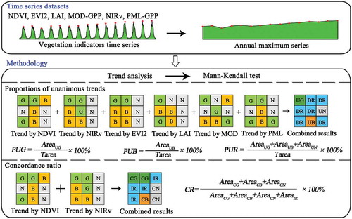
1.2.2. Trend analysis of vegetation indicators and climatic variables

A non-parametric Mann–Kendall test was used to conduct per-pixel trend analyses (Kendall 1975). The Mann-Kendall trend test can detect a long-term trend without the requirements of independence and normality. The test statistic Z was calculated as:

(1) $Z=\left\{\begin{array}{c}\frac{S-1}{\sqrt{Var(S)}},S>0\\ 0,S=0\\ \frac{S+1}{\sqrt{Var(S)}},S<0\end{array}\right.,S=\sum _{i=1}^{n-1}\hspace{0.17em}\sum _{k=i+1}^n(sign(xk-xi)),Var\left(S\right)=\frac{n\left(n-1\right)\left(2n+5\right)}{18},sign(xk-xi)=\left\{\begin{array}{c}1,xk-xi>0\\ 0,xk-xi=0\\ -1,xk-xi<0\end{array}\right.$(1)

where n is the length of time series, x_k and x_i are the vegetation indicator values at times k and i (k > i), and sign(x_k-x_i) is the symbolic function. Z values that are higher or lower than 0 indicate an increasing or decreasing trend, respectively. The significance level of 10% was applied in recent studies (Chen et al. 2019; Murthy and Bagchi 2018) and used here. If Z was greater than 1.64 or lower than −1.64, we concluded that there was a significant positive or negative trend in the time series; otherwise, there was no significant trend.

Trend analysis was conducted for six vegetation indicator and two climatic variables globally through a per-pixel strategy. Significant positive or negative trends in the vegetation indicator corresponded to greening or browning, respectively. The percentage of greening or browning was estimated as all areas showing a significant increasing or decreasing trend divided by the total vegetated area and this was multiplied by 100, respectively. The net greening was calculated as the percentage of greening minus the percentage of browning at the global scale and for a specific region/biomes.

1.2.3. Proportions of unanimous trends estimated by six indicators and their relationships with change magnitudes

Unanimous results were obtained when the estimated trends by six indicators were unanimous in one pixel, which could be unanimous greening, unanimous browning or unanimous no trend. Otherwise, the types of discrepancies and the primary contributors were further evaluated. For example, if greening was only revealed by NDVI in contrast to no trends by other five indicators, the primary contributor to the discrepancy was NDVI. The proportion of unanimous greening or unanimous browning in vegetated areas was computed at the global and the country levels. Net changes were also calculated at country level, which were estimated as the total areas of unanimous greening pixels minus unanimous browning pixels. The proportion of Unanimous Greening (PUG), Unanimous Browning (PUB) or Unanimous Results (PUR) was computed as follows (equation (2)(2) $PUG=\frac{Are{a}_{UG}}{Tarea}\times 100\mathrm{\%};PUB=\frac{Are{a}_{UB}}{Tarea}\times 100\mathrm{\%};PUR=\frac{Are{a}_{UG}+Are{a}_{UB}+Are{a}_{UN}}{Tarea}\times 100\mathrm{\%}$(2) ).

(2) $PUG=\frac{Are{a}_{UG}}{Tarea}\times 100\mathrm{\%};PUB=\frac{Are{a}_{UB}}{Tarea}\times 100\mathrm{\%};PUR=\frac{Are{a}_{UG}+Are{a}_{UB}+Are{a}_{UN}}{Tarea}\times 100\mathrm{\%}$(2)

where Area_UG, Area_UB, Area_UN, indicate the areas with unanimous greening, unanimous browning and unanimous no trend, respectively; Tarea represents the total area (Figure 1).

For each vegetation indicator, the change magnitudes and their corresponding proportions of unanimous results were investigated. Change magnitudes were calculated based on an ordinary linear regression (OLS) model against time. The OLS models instead of the Generalized Least Square (GLS) regression were applied for this purpose since a majority sites (84–90%) among randomly selected 720 sampling sites distributed globally did not show temporal auto-correlation in the residuals of the OLS models (Figure S1). The change magnitudes were computed to facilitate the comparability of trends between sensors and indicators (Brandt et al. 2018b). For each vegetation indicator, the change magnitudes per pixel were computed as the relative changes in percent: the slope multiplied with the number of years and divided by the mean.

(3) $Changemagnitude=Slope\times N_{year}/Mean\times 100\mathrm{\%}$(3)

Where slope is derived from the linear regression model, Mean is the average value of the annual maximum in the vegetation indicator time series (2003–2017). N_year is the length of the study period which is 14.

1.2.4. Concordance ratio in estimated trends by each pair of indicators and discrepancy due to changes in climate

Concordance Ratio (CR) in estimated trends was designed to measure the percentages of consistent-estimated trends by two pairs of indicators (Figure 1). Consistent-estimated trends were determined when the two indicators agreed with each other, which could be consistent greening, browning, or no trend. Higher values in concordance ratio signify better consistency in estimated trends in peak growth from two indicators.

(4) $CR=\frac{Are{a}_{CG}+Are{a}_{CB}+Are{a}_{CN}}{Are{a}_{CG}+Are{a}_{CB}+Are{a}_{CN}+Are{a}_{IR}}\times 100\mathrm{\%}$(4)

Where Area_CG, Area_CB, Area_CN, Area_IR indicate the areas with consistent greening, consistent browning, consistent no trends and inconsistent results when estimated by the two indicators (Figure 1).

The concordance ratio was computed for each pair of six indicators at the global scale and across different biomes. In order to explore the possible influence of climate, the concordance ratios under different climatic conditions such as warming, cooling, wetting, and drying were also calculated for each pair of six indicators. Additionally, the relationships between vegetation trends estimated from each indicator and their corresponding changes in climatic conditions were investigated. The slopes of trends in climatic variables (temperature, precipitation) were calculated based on linear regression models with time as the independent variable to indicate the changes in climate conditions. The possible discrepancies in sensitivity to different climatic conditions among these six indicators were further investigated based on the corresponding boxplots of vegetation trends under different ranges of trends in temperature and precipitation. For example, if there was a close association between drying and browning revealed by NDVI instead of by PML-GPP, the boxplot of browning would be located primarily in the drying condition when estimated by NDVI, but that by PML-GPP would not. Otherwise, if browning estimated by either NDVI or PML-GPP had no tendency with changes in precipitation (wetting or drying), their frequency distributions of browning indicated by the boxplots would be similar to that of precipitation changes (drying and wetting conditions).

3. Results

3.1. Global greening or browning estimated by six vegetation indicators

Greening ranged from 12 to 24% of the vegetated areas at the global scale when estimated with these six indicators (Figure 2). Specifically, greening was experienced in 12.05, 15.36, 16.29, 20.75, 22.05, and 23.39% of the vegetated areas when estimated from LAI, NIRv, EVI2, MOD-GPP, PML-GPP and NDVI, respectively (Figure 2). Browning was experienced in around 4–6% of the vegetated area when estimated by four greenness indices (NDVI, EVI2, NIRv and LAI). However, 13.45% of the vegetated area experienced browning according to PML-GPP, in contrast to only 2.08% by MODIS GPP (Figure 2). NDVI and MOD-GPP revealed more greening and less browning compared to other indicators. Net greening estimated by NDVI or MOD-GPP was around 19% in contrast to only 8–11% estimated by other four indicators (Figure 2).

Figure 2. Maps of trends in six vegetation indicators (a-f), and the corresponding greening, browning, and net greening (g-i)

Notes: ENF, EBF, DNF, DBF, MF, and OWV represented the evergreen needle-leaf forest, evergreen broad-leaf forest, deciduous needle-leaf forest, deciduous broad-leaf forest, mixed forest, and other woody vegetation, respectively. MOD and PML denoted the MOD-GPP and PML-GPP, respectively.

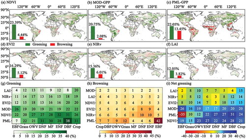
Greening varied significantly among different biomes when estimated by six indicators (Figure 2). For example, greening was experienced in around 40% of the Deciduous Broad-leaf Forest (DBF) in contrast to less than 10% of the Evergreen Broad-leaf Forest (EBF) when estimated by PML-GPP. Greening of mixed forests and deciduous broad-leaf forest was estimated to be less than 10% by LAI compared to around 30% or higher by two GPP products (Figure 2). Browning among different biomes was much more consistent compared to greening except for the PML-GPP (Figure 2). Browning ranged from 1 to 10% among different biomes when estimated by all indicators except PML-GPP. Browning in evergreen broad-leaf forest was very conspicuous (over 40%) when revealed by PML-GPP (Figure 2). Therefore, net greening in evergreen broad-leaf forest was negative when revealed by PML-GPP (Figure 2). Apart from PML-GPP, net greening among different biomes varied from 2% to around 30% depending on the indicator applied (Figure 2). For example, net greening in cropland ranged from 14% to 24% when revealed by the six indicators. If vegetation trends revealed by any of these six vegetation indicators were taken into account, roughly one-half (48.72%) or one-fifth (20.96%) of the vegetated area experienced greening or browning in peak vegetation growth, respectively.

3.2. Hotspots of unanimous results and major discrepancies from six indicators

Around two-fifths (38.71%) of global-vegetated area yielded unanimous results from the six vegetation indicators (Figure 3, Figure S1, Figure S5-8). Specifically, unanimous greening was exhibited in only around 2% (2.31%) of the vegetated area. Unanimous greening was scattered primarily in the northern Hemisphere (Figure 3, Figure S1). Unanimous greening was mainly found in non-forest biomes: grassland (44.64%), cropland (25.33%) and other woody vegetation (26.18%) (Figure S1). The forest biome contributed to less than 4% of unanimous greening, although accounted for over 20% of the vegetated area (Figure S1). Seven hotspots of unanimous greening have been highlighted (Figure 3, Figure S1): three located in northern high latitudes (Eastern Russia, Canada, and Alaska); two in mid northern latitudes (China and Turkey); one in low northern latitudes (India); and one in the Southern Hemisphere (Southern Brazil) (Figure S1, Figure S5-6, Figure S15).

Figure 3. (a) Maps of proportions of unanimous greening, (b) and browning at country level, (c) probability distribution of change magnitudes; (d) and their associations with proportion of unanimous results; (e) net changes at country level; (f) major discrepancy

Notes: “MOD-GPP↑” denoted an increasing trend from MOD-GPP versus no trends from other vegetation indicators. “PML-GPP↓” represented a decreasing trend in peak vegetation growth from PML-GPP versus no trends from other vegetation indicators, etc.

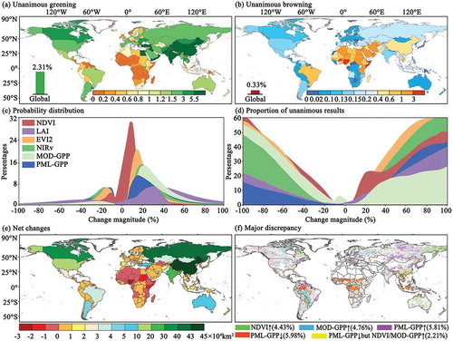
There was 0.33% of the vegetated area with unanimous browning, mainly scattered in the tropics (Figure 3, Figure S1). Similar to unanimous greening, unanimous browning was mainly found in non-forest biomes: grassland (65.19%) and other woody vegetation (25.53%). Unanimous no trend was found in 36.07% of the vegetated area, principally located in Asia (central Asia and northern Asia), Australia, Southern Africa, Southern North America, and the Amazon region. Three hotspots of unanimous browning were highlighted: the Sahel region, southeast edge of Amazon and the Yangtze River Delta in China (Eastern China) (Figure S1, Figure S16).

Most hotspots of unanimous greening (5 out 7) were associated with emerging economies (Table S2). China alone accounted for one-fifth of unanimous greening in vegetated areas. Most hotspots of unanimous greening were confirmed from the net changes at the country level except the one in Brazil (Figure 3). Unanimous browning in the Sahel region was also highlighted by the corresponding net changes (Figure 3). The five top countries with net changes in unanimous results were China, Russia, Canada, India, and the United States (Figure 3, Table S2).

The proportions of unanimous results gradually increased with the change magnitude of vegetation indicators (Figure 3). For example, the proportion of unanimous results was around or above 50% when the absolute values of the change magnitudes were close to 100%. However, the proportion of unanimous results was around 10% or less when the change magnitudes of vegetation indicators were 20%. The change magnitudes varied among these six indicators: the NDVI showed the smallest change magnitudes versus the most outstanding change magnitudes from LAI. For a specific change magnitude, the corresponding proportions of unanimous results exhibited the lowest values in either MOD-GPP (in the case of positive change magnitudes) or PML-GPP (Figure 3).

Discrepancies in the vegetation trends were exhibited by a majority (61.29%) of the vegetated area when all six indicators were considered (Figure 3, Figure S4, Figure S 9–14, and Table S3). There were three types of discrepancies. The first type of discrepancy was greening estimated from only some indicators versus no trends in others (greening vs no trend), which occurred in two fifths (40.66%) of the vegetated areas (Table S3). For example, 5.81, 4.76, and 4.43% of global-vegetated areas showed greening estimated only by the PML-GPP (mainly located in Eurasia), MOD-GPP (mainly in the middle of South American and North America) or NDVI (principally distributed in northern high latitude), respectively (Figure 3). The second type of discrepancy was browning from only some indicators versus no trends in others (browning vs no trend, Table S3), which was shown in 14.88% vegetated areas. Especially, the tropical region was characterized as browning only by PML-GPP (5.98% global-vegetated area). The third type of discrepancy was contradictory results (greening vs browning) by these indicators (Table S3), which were shown in 5.75% of the vegetated areas. Specifically, around 2.21% of the vegetated areas showed greening by MOD-GPP or NDVI versus browning by PML-GPP, mainly distributed in the tropics (Figure 3).

3.3. Concordance ratio between each pair of 6 indicators and possible associations with climatic conditions

The concordance ratio for the estimated trends varied significantly among each pair of 6 indicators (Figure 4). At the global scale, the highest concordance ratio was obtained for EVI2 and NIRv (>94%) and the lowest concordance ratio was exhibited between PML-GPP and other indicators. Apart from the pair of EVI2 and NIRv, the concordance ratio at the global scale between different indicators was around 72–75%, with higher values from each pair of four radiometric indices and not for the two GPP products. Specifically, the concordance ratio between PML-GPP and other indicators was no more than 65% at the global scale. Compared with the other 3 radiometric indices, LAI showed a slightly higher concordance ratio with two GPP products. A very high concordance ratio between EVI2 and NIRv was consistently confirmed across different vegetation types (Figure 4). Apart from the pair of EVI2 and NIRv, the concordance ratios were dependent on vegetation types: higher in cropland and lower in forestland. Specifically, the concordance ratios was 51–62% in deciduous needle-leaf forest between each pair of 6 indicators except for the pair of EVI2 and NIRv, and 37–49% in evergreen broadleaf forest between PML-GPP and other indicators (Figure 4).

Figure 4. (a) Concordance ratios between different indicators at the global scale; (b) and under changes in climate; (c) boxplots of greening and browning under changes in climate (warming or cooling conditions, wetting or drying)

Notes: In Figure 4(a), ENF, EBF, DNF, DBF, MF, and OWV represented the evergreen needle-leaf forest, evergreen broad-leaf forest, deciduous needle-leaf forest, deciduous broad-leaf forest, mixed forest, and other woody vegetation, respectively. MOD and PML denoted the MOD-GPP and PML-GPP, respectively. In Figure 4(b), the global average values in each pair of indicators were shaded in gray. In Figure 4(c), the white line parallel to the x-axis represented the medium level of changes in climatic variables.

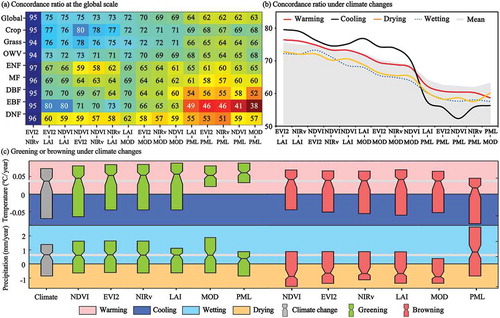
The concordance ratios between EVI2 and NIRv were consistently high (>93%) under changes in climatic conditions (warming, cooling, wetting, and drying) (Figure S3). At the global scale the concordance ratio between each pair of 6 indicators except PML-GPP was higher during cooling conditions compared to warming conditions. The concordance ratio was lower during wetting and drying conditions compared to warming conditions. The concordance ratios between PML-GPP and other indicators during changes in temperature and precipitation (warming, cooling, wetting, and drying) was lower than the global average (Figure 4). The concordance ratios under different climatic conditions were further analyzed for different biomes (Figure 4, Figure S2). The concordance ratios between PML-GPP and other indicators under wetting conditions were distinctively higher or lower than those under drying conditions depending on the biome types: higher in Evergreen forest and lower in mixed forest (Figure S2).

There was much more warming and slightly more wetting compared to cooling and drying at the global scale (Figure 4). Specifically, there were 12.08, 9.55, 6.89, and 6.78% of the vegetated areas showing warming, wetting, cooling, and drying, respectively (Figure S1). Greening was more pronounced during warming conditions for the GPP products when compared with the greenness indices (Figure 4). There was no obvious association between browning and cooling conditions for most indicators except PML-GPP (Figure 4). Browning tended to be associated with drying by most indicators, in contrast to wetting by PML-GPP product (Figure 4). Forestland showed diverse responses to changes in climatic conditions revealed by these six indicators (Figure S2). For example, evergreen needle-leaf forests (ENF) under warming conditions showed more greening by LAI and two GPP products. The evergreen broad-leaf forest (EBF) under warming conditions showed obvious browning by most indicators excluding the PML-GPP. The coupling of browning and wetting conditions was typically found in EBF, mixed forest, and other woody vegetation revealed by PML-GPP (Figure S3).

3.4. Consistency and discrepancies across different latitudes

The inter-annual variations of six vegetation indicators were investigated across different latitudes. For each indicator, the original time series datasets were normalized by subtracting the mean and then dividing by its standard deviation. The temporal profiles of six indicators together with two climatic variables were assessed at the global scale and across different latitudes (Figure 5). At the global scale, discrepancies were observed in their extremes (Figure 5). For example, NDVI was at its maximum in 2015, accompanied by local minimum from other vegetation indicators. The minima of all vegetation indicators were shownin the early 2000s except for LAI (2009). Vegetation indicators demonstrated different responses to climatic extremes in the following three aspects: the change directions (increase or decrease), change magnitudes, and recovery speed (rapidly or slowly after climatic extremes) (Figure 5, Figure S15-16).

Figure 5. Inter-annual variations of six vegetation indicators and climatic variables globally (a) and across different latitudes (c-f)

Notes: In order to facilitate the comparability between different indicators, the original annual time series of six vegetation indicators were normalized through subtracting the mean divided by its corresponding standard derivations. The gray area indicates the mean values of six indicators. Some abnormal years with climatic extremes were highlighted in pink.

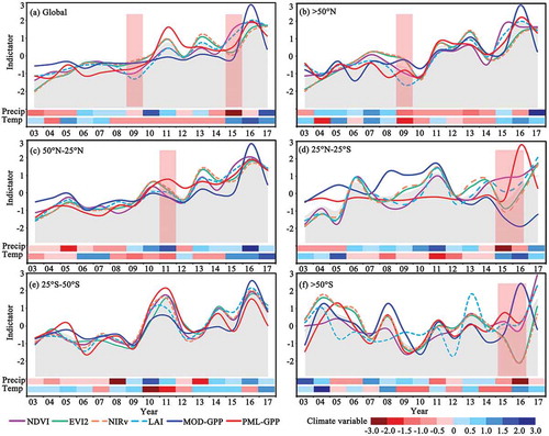
In equatorial regions, discrepancies were primarily attributed to the excess changes of two GPP products and opposite change directions of NDVI to climatic extremes (Figure 5). PML-GPP exhibited a remarkable decrease during El Niño (2015–2016) and it took longer periods to recover (Figure 5). Long recovery from drought stress in tropics has recently been reported in a study based on FLUXNET data and GPP products (Schwalm et al. 2017). However, MOD-GPP and NDVI increased during a strong El Niño (2015–2016). Saturation of NDVI in dense canopies and insensibility to declines of photosynthesis during climatic extremes might account for the different patterns (Huang et al. 2018).

In high southern latitude, differences in these vegetation indicators were shown in their change directions and magnitudes during climatic extremes as well as the normal years (Figure 5). Most indicators declined during a strong El Niño (2015–2016) except MOD-GPP (significant increase). The two GPP products showed larger inter-annual variations compared to other indicators. Specifically, PML-GPP significantly increased during slightly cold years (i.e., 2015) or some normal years (i.e. 2005). The differences shown by these vegetation indicators in northern high latitude were similar to those in southern high latitude (Figure 5). For example, two GPP products increased during abnormal drought and cold climate (2009), whereas four radiometric indices (NDVI, EVI2, LAI, and NIRv) decreased under these conditions (Figure 5). Higher consistency among these six vegetation indicators was shown in the medium latitudes compared to those in the tropics and higher latitudes (Figure 5).

4. Discussions

4.1. Significances of unanimous results estimated from six indicators

We reported the first systematic evaluation of the consistencies and discrepancies of changes in peak vegetation growth revealed by six different vegetation indicators based on 8-day composite time series datasets with a spatial resolution of 500 m for the recent past two decades. New data with finer spatio-temporal resolution will inform analyses of historic greening trends (Myers-Smith et al. 2020). Our comparative investigation provides a knowledge base to understand the long-term response of global peak vegetation growth under changes in climatic conditions.

We found that the concordance ratio between each pair of six vegetation indicators gradually increased with their corresponding change magnitudes. A distribution map of unanimous results provided valuable information on trends in vegetation productivity, which could be taken as ground truth data (Figure S5-8, Table S4). Comprehensive analysis using multiple indicators contributes to better understanding of vegetation dynamics (Andela et al. 2013). Unanimous greening in China and India (Figure 3) was confirmed extensively by recent studies with high confidence (Piao et al. 2020; Shukla et al. 2019). There were no hotspots with unanimous greening in Africa and Oceania.

Browning has been extensively evidenced in the tropics and the southern hemisphere in recent studies (De Jong et al. 2012; Zhang et al. 2017a). Unanimous browning in the southeast edge of Amazon could be associated with the well-documented deforestation (Song et al. 2018). Urbanization was responsible for unanimous browning in Yangtze River Delta in China (Qiu et al. 2019, 2020; Song et al. 2018). Extensive studies have demonstrated the precipitation-driven re-greening over the Sahel (Brandt et al. 2015). However, there were still large areas in the Sahel showing unanimous browning, which indicates the spatio-temporal complexity in the climate conditions and land cover in the Sahel (Brandt et al. 2018a).

4.2. Consistency in vegetation greening assessment among 6 indicators

The first hypothesis was not supported in this study. The highest concordance ratio in estimated trends was shown between EVI2 and NIRv (>95%). Apart from the pair of EVI2 and NIRv, the concordance ratios between each pair of six indicators were less than 80%: approximately 72–75% between NDVI and other radiometric indices (EVI2, LAI, NIRv); around 62–73% between GPP products and radiometric indices (NDVI, EVI2, LAI, NIRv) (Figure 4). Apart from EVI2 and NIRv, the concordance ratios between different indicators varied significantly among different biomes: higher in cropland and lower in forestland (Figure 4). The absolute difference in estimated global greening by different vegetation indicators could be larger than 10% at the global scale (i.e., greening in 23% of the vegetated areas estimated using NDVI versus only 12% of the vegetated areas estimated using LAI).

This study systematically investigated the consistency and discrepancies of global greening in peak growth estimated by the NDVI, EVI2, LAI, and MOD-GPP together with two newly developed indicators, NIRv and PML-GPP. This study found that the widely applied NDVI showed less than 80% concordance with other indicators and almost doubled the amplitudes of global net greening compared to other four indicators (EVI2, LAI, NIRv, and PML-GPP). These findings suggest that the discrepancy of estimated greening by different indicators is far greater than the well-documented decoupling of GPP and vegetation indices in the tropics (Piao et al. 2020; Yang et al. 2018; Zhao and Running 2010).

4.3. Extent of consistency vary depending on climatic conditions

The second hypothesis was supported by this study. Different sensitivities to changes in climatic conditions were revealed by the six vegetation indicators. This informs our understanding of the possible consequences of climatic stress (Stocker et al. 2019). Browning in evergreen forest under warming condition might be associated with the possible intensified drought stress by heat (Lee et al. 2013), which was revealed by all vegetation indicators except the PML-GPP (Figure S2). Extreme climatic events such as the drought are the key drivers of recent browning and are reported to be increasing over the twentieth centuries (Treharne et al. 2019). However, the impacts of extreme climatic events were underestimated by satellite monitoring (Schwalm et al. 2017; Stocker et al. 2019). This study found that these two GPP products (PML-GPP, MOD-GPP) generally exhibited greater change magnitudes and took longer periods to recover than vegetation indices during climatic extremes (Figure 5, Figure S9-16). The findings in this study and a recent study based on 12 remote sensing-based modeled GPP (Sun et al. 2019) indicate that GPP products validated with FLUXNET data (limited coverages, mainly distributed in North America and Europe) might not be reliable for its global applications in exploring vegetation sensibility to climatic changes.

4.4. Implications and future works

We propose careful applications of MOD-GPP and NDVI for exploring changes in peak vegetation growth during the 2015–16 period, given their consistently high values across different latitudes during a strong El Niño (2015–2016) (Figure S18-35). Therefore, global greening by NDVI and MOD-GPP was shown in over 20% of vegetated area, which was much higher than the other three vegetation indices. The risk of overestimating the availability and productive potential of these areas is large, as it may divert attention from efforts to reduce the demand for land-intensive commodities (Gibbs and Salmon 2015). We suggest applications of PML-GPP with caution in northern hemisphere and the tropics compared with MOD-GPP. Here are the suggestions for applications in exploring peak vegetation growth: MOD-GPP (universal peak in 2016), PML-GPP (more validation in tropics and northern Hemisphere), and all proxies (caution during climatic extremes).

Regarding the most region displaying the greatest discrepancies (the tropics)/biome (EBF), more attention should be paid to inter-annual variation or short-term changes during climatic extremes. Accounting for trends should be emphasized when analyzing long-term vegetation proxy time series (De Jong et al. 2012). Time series models with seasonal and inter-annual components could be considered in future work, such as the Breaks For Additive Seasonal and Trend (BFAST) (Forkel et al. 2013; Verbesselt et al. 2010). Generalized additive-mixed model (GAMM) with a temporal autocorrelated error structure (ARMA) could be applied to further determine if there are any significant relationships between the inconsistency of these indicators and possible drivers (temperature, precipitation, and carbon dioxide concentration) for each biome, for the different regions and globally. An ensemble evaluation using different input datasets provides more comprehensive quantification of uncertainty and errors in space and time (Burrell, Evans, and Liu 2018).

5. Conclusions

We reported the first systematic investigation on the impact of vegetation indicator selection on global greening in peak growth by six indicators (NDVI, EVI2, NIRv, LAI, MOD-GPP, and PML-GPP) at the global scale. We found that these two commonly applied indicators, NDVI, and MOD-GPP, produced much more net greening compared to others. Higher consistency was always observed between EVI2 and NIRv (>94%), instead of between NDVI and other vegetation indices. The concordance ratio between each pair of six vegetation indicators gradually increased with their corresponding change magnitudes. Unanimous greening or browning estimated by these six indicators was detected in 2.31 or 0.33% of the vegetated area, respectively. Widespread discrepancies (61% vegetated area) were associated with different sensitivities to changes in climatic conditions. Greening was pronounced during warming conditions for the GPP products when compared with the greenness indices. At the global scale the concordance ratio was higher during cooling periods among all the indicators except between PML-GPP compared to warming conditions. There was more browning during drying periods when estimated by all indicators except the PML-GPP. We emphasize the applications of multiple indicators, especially the newly available products, for the purpose of comprehensive quantification of vegetation productivity. Datasets supporing these findings are available online at https://github.com/FuzhouSIRC/Greening_6indicators.

Acknowledgements

This work was supported by the National Natural Science Foundation of China (grant no. 41771468, 41471362), funding from the Science Bureau of Fujian Province (2020N5002) and Fuzhou University (GD1805), the scholarship under the China Scholarship Council (CSC) (201806655006). We are very grateful to the editors and anonymous reviewers for offering insightful suggestions and detailed comments which significantly improve the manuscript. Thank Jennifer Johnson from the Department of Global Ecology, Carnegie Institution for Science, for helping us improving the language.

Disclosure statement

No potential conflict of interest was reported by the authors.

Supplemental data

Supplemental data for this article can be accessed here.

Additional information

Funding

This work was supported by the National Natural Science Foundation of China (grant no. 41771468, 41471362) and the Science Bureau of Fujian Province (2020N5002).

References

- Alcaraz‐Segura, D., E. Chuvieco, H. E. Epstein, E. S. Kasischke, and A. Trishchenko. 2010. “Debating the Greening Vs. Browning of the North American Boreal Forest: Differences between Satellite Datasets.” Global Change Biol 16: 760–770. doi:10.1111/j.1365-2486.2009.01956.x.
- Andela, N., Y. Liu, A. Van Dijk, R. De Jeu, and T. McVicar. 2013. “Global Changes in Dryland Vegetation Dynamics (1988-2008) Assessed by Satellite Remote Sensing: Comparing a New Passive Microwave Vegetation Density Record with Reflective Greenness Data.” Biogeosciences 10 (10): 6657–6676.
- Badgley, G., C. B. Field, and J. A. Berry. 2017. “Canopy Near-infrared Reflectance and Terrestrial Photosynthesis.” Science Advances 3: e1602244. doi:10.1126/sciadv.1602244.
- Badgley, G., L. D. L. Anderegg, J. A. Berry, and C. B. Field. 2019. “Terrestrial Gross Primary Production: Using NIRV to Scale from Site to Globe.” Global Change Biol 25: 3731–3740. doi:10.1111/gcb.14729.
- Beck, H. E., T. R. McVicar, A. I. J. M. van Dijk, J. Schellekens, R. A. M. de Jeu, and L. A. Bruijnzeel. 2011. “Global Evaluation of Four AVHRR–NDVI Data Sets: Intercomparison and Assessment against Landsat Imagery.” Remote Sensing of Environment 115: 2547–2563. doi:10.1016/j.rse.2011.05.012.
- Bianchi, E., R. Villalba, and A. Solarte. 2020. “NDVI Spatio-temporal Patterns and Climatic Controls over Northern Patagonia.” Ecosystems 23: 84–97. doi:10.1007/s10021-019-00389-3.
- Brandt, M., C. Mbow, A. A. Diouf, A. Verger, C. Samimi, and R. Fensholt. 2015. “Ground- and Satellite-based Evidence of the Biophysical Mechanisms behind the Greening Sahel.” Global Change Biol 21: 1610–1620. doi:10.1111/gcb.12807.
- Brandt, M., K. Rasmussen, P. Hiernaux, S. Herrmann, C. J. Tucker, X. Tong, F. Tian, et al. 2018a. “Reduction of Tree Cover in West African Woodlands and Promotion in Semi-arid Farmlands.” Nature Geoscience 11: 328–333. doi:10.1038/s41561-018-0092-x.
- Brandt, M., Y. Yue, J. P. Wigneron, X. Tong, F. Tian, M. R. Jepsen, X. Xiao, et al. 2018b. “Satellite-Observed Major Greening and Biomass Increase in South China Karst during Recent Decade.” Earth’s Future 6: 1017–1028. doi:10.1029/2018EF000890.
- Burrell, A. L., J. P. Evans, and Y. Liu. 2018. “The Impact of Dataset Selection on Land Degradation Assessment.” Isprs J Photogramm 146: 22–37.
- Chen, C., T. Park, X. Wang, S. Piao, B. Xu, R. K. Chaturvedi, R. Fuchs, et al. 2019. “China and India Lead in Greening of the World through Land-use Management.” Nature Sustainability 2: 122–129. doi:10.1038/s41893-019-0220-7.
- De Jong, R., J. Verbesselt, M. E. Schaepman, and S. De Bruin. 2012. “Trend Changes in Global Greening and Browning: Contribution of Short-term Trends to Longer-term Change.” Global Change Biol 18: 642–655. doi:10.1111/j.1365-2486.2011.02578.x.
- Evans, J., and R. Geerken. 2004. “Discrimination between Climate and Human-induced Dryland Degradation.” Journal of Arid Environments 57: 535–554. doi:10.1016/S0140-1963(03)00121-6.
- Forkel, M., N. Carvalhais, J. Verbesselt, M. D. Mahecha, C. S. R. Neigh, and M. Reichstein. 2013. “Trend Change Detection in NDVI Time Series: Effects of Inter-annual Variability and Methodology.” Remote Sensing 5: 2113–2144. doi:10.3390/rs5052113.
- Gibbs, H. K., and J. M. Salmon. 2015. “Mapping the World’s Degraded Lands.” Applied Geography 57: 12–21. doi:10.1016/j.apgeog.2014.11.024.
- Heinsch, F. A., H. Hashimoto, M. Zhao, M. Reeves, R. R. Nemani, and S. W. Running. 2004. “A Continuous Satellite-Derived Measure of Global Terrestrial Primary Production.” Bioscience 54: 547–560. doi:10.1641/0006-3568(2004)054[0547:ACSMOG]2.0.CO;2.
- Huang, K., J. Xia, Y. Wang, A. Ahlström, J. Chen, R. B. Cook, E. Cui, et al. 2018. “Enhanced Peak Growth of Global Vegetation and Its Key Mechanisms.” Nature Ecology & Evolution 2: 1897–1905. doi:10.1038/s41559-018-0714-0.
- Jiang, C., Y. Ryu, H. Fang, R. Myneni, M. Claverie, and Z. Zhu. 2017. “Inconsistencies of Interannual Variability and Trends in Long-term Satellite Leaf Area Index Products.” Global Change Biol 23: 4133–4146. doi:10.1111/gcb.13787.
- Jiang, Z., A. R. Huete, K. Didan, and T. Miura. 2008. “Development of a Two-band Enhanced Vegetation Index without a Blue Band.” Remote Sensing of Environment 112: 3833–3845. doi:10.1016/j.rse.2008.06.006.
- Kendall, M. G. 1975. Rank Correlation Methods. London: Griffin.
- Lee, J.-E., C. Frankenberg, C. van der Tol, J. A. Berry, L. Guanter, C. K. Boyce, J. B. Fisher, E. Morrow, J. R. Worden, and S. Asefi. 2013. “Forest Productivity and Water Stress in Amazonia: Observations from GOSAT Chlorophyll Fluorescence.” Proceedings of the Royal Society B: Biological Sciences 280: 20130171. doi:10.1098/rspb.2013.0171.
- McNally, A., K. Arsenault, S. Kumar, S. Shukla, P. Peterson, S. Wang, C. Funk, C. D. Peters-Lidard, and J. P. Verdin. 2017. “A Land Data Assimilation System for sub-Saharan Africa Food and Water Security Applications.” Scientific Data 4: 170012. doi:10.1038/sdata.2017.12.
- Murthy, K., and S. Bagchi. 2018. “Spatial Patterns of Long‐term Vegetation Greening and Browning are Consistent across Multiple Scales: Implications for Monitoring Land Degradation.” Land Degrad Dev 29: 2485–2495. doi:10.1002/ldr.3019.
- Myers-Smith, I. H., J. T. Kerby, G. K. Phoenix, J. W. Bjerke, H. E. Epstein, J. J. Assmann, C. John, L. Andreu-Hayles, S. Angers-Blondin, and P. S. Beck. 2020. “Complexity Revealed in the Greening of the Arctic.” Nature Climate Change 10: 106–117. doi:10.1038/s41558-019-0688-1.
- Myneni, R. B., F. G. Hall, P. J. Sellers, and A. L. Marshak. 1995. “The Interpretation of Spectral Vegetation Indexes.” Ieee T Geosci Remote 33: 481–486. doi:10.1109/TGRS.1995.8746029.
- Park, T., C. Chen, M. Macias-Fauria, H. Tømmervik, S. Choi, A. Winkler, U. S. Bhatt, et al. 2019. “Changes in Timing of Seasonal Peak Photosynthetic Activity in Northern Ecosystems.” Global Change Biology 25 (7): 2382–2395. doi:10.1111/gcb.14638.
- Pettorelli, N., J. O. Vik, A. Mysterud, J.-M. Gaillard, C. J. Tucker, and N. C. Stenseth. 2005. “Using the Satellite-derived NDVI to Assess Ecological Responses to Environmental Change.” Trends In Ecology & Evolution 20 (9): 503–510.
- Piao, S., X. Wang, T. Park, C. Chen, X. Lian, Y. He, J. W. Bjerke, et al. 2020. “Characteristics, Drivers and Feedbacks of Global Greening.” Nature Reviews Earth & Environment 1: 14–27. doi:10.1038/s43017-019-0001-x.
- Qiu, B., H. Li, C. Chen, Z. Tang, K. Zhang, and J. Berry. 2019. “Tracking Spatial-temporal Landscape Changes of Impervious Surface Areas, Bare Lands, and Inundation Areas in China during 2001-2017.” Land Degradation & Development 0 (ja). doi: 10.1002/ldr.3352.
- Qiu, B., H. Li, Z. Tang, C. Chen, and J. Berry. 2020. “How Cropland Losses Shaped by Unbalanced Urbanization Process?” Land Use Policy 96: 104715. doi:10.1016/j.landusepol.2020.104715.
- Qiu, B., M. Feng, and Z. Tang. 2016. “A Simple Smoother Based on Continuous Wavelet Transform: Comparative Evaluation Based on the Fidelity, Smoothness and Efficiency in Phenological Estimation.” Int. J. Appl. Earth. Obs. 47: 91–101. doi:10.1016/j.jag.2015.11.009.
- Scheftic, W., X. Zeng, P. Broxton, and M. Brunke. 2014. “Intercomparison of Seven NDVI Products over the United States and Mexico.” Remote Sensing 6: 1057–1084. doi:10.3390/rs6021057.
- Schwalm, C. R., W. R. L. Anderegg, A. M. Michalak, J. B. Fisher, F. Biondi, G. Koch, M. Litvak, et al. 2017. “Global Patterns of Drought Recovery.” Nature 548: 202. doi:10.1038/nature23021.
- Shukla, J. S., E. Calvo Buendia, V. Masson-Delmotte, H.-O. Pörtner, D. C. Roberts, P. Zhai, R. Slade, et al. (Eds.). 2019. Climate Change and Land: an IPCC Special Report on Climate Change, Desertification, Land Degradation, Sustainable Land Management, Food Security, and Greenhouse Gas Fluxes in Terrestrial Ecosystems. Geneva, Switzerland: IPCC.
- Song, X.-P., M. C. Hansen, S. V. Stehman, P. V. Potapov, A. Tyukavina, E. F. Vermote, and J. R. Townshend. 2018. “Global Land Change from 1982 to 2016.” Nature 560: 639–643. doi:10.1038/s41586-018-0411-9.
- Stocker, B. D., J. Zscheischler, T. F. Keenan, I. C. Prentice, S. I. Seneviratne, and J. Peñuelas. 2019. “Drought Impacts on Terrestrial Primary Production Underestimated by Satellite Monitoring.” Nature Geoscience 12: 264–270. doi:10.1038/s41561-019-0318-6.
- Sun, Z., X. Wang, X. Zhang, H. Tani, E. Guo, S. Yin, and T. Zhang. 2019. “Evaluating and Comparing Remote Sensing Terrestrial GPP Models for Their Response to Climate Variability and CO2 Trends.” The Science of the Total Environment 668: 696–713. doi:10.1016/j.scitotenv.2019.03.025.
- Tramontana, G., M. Jung, C. R. Schwalm, K. Ichii, G. Camps-Valls, B. Ráduly, M. Reichstein, et al. 2016. “Predicting Carbon Dioxide and Energy Fluxes across Global FLUXNET Sites with Regression Algorithms.” Biogeosciences 13: 4291–4313. doi:10.5194/bg-13-4291-2016.
- Treharne, R., J. W. Bjerke, H. Tømmervik, L. Stendardi, and G. K. Phoenix. 2019. “Arctic Browning: Impacts of Extreme Climatic Events on Heathland Ecosystem CO2 Fluxes.” Global Change Biol 25: 489–503. doi:10.1111/gcb.14500.
- Verbesselt, J., R. Hyndman, G. Newnham, and D. Culvenor. 2010. “Detecting Trend and Seasonal Changes in Satellite Image Time Series.” Remote Sensing of Environment 114: 106–115. doi:10.1016/j.rse.2009.08.014.
- Verbyla, D. 2008. “The Greening and Browning of Alaska Based on 1982–2003 Satellite Data.” Global Ecol Biogeogr 17: 547–555. doi:10.1111/j.1466-8238.2008.00396.x.
- Yang, J., H. Tian, S. Pan, G. Chen, B. Zhang, and S. Dangal. 2018. “Amazon Drought and Forest Response: Largely Reduced Forest Photosynthesis but Slightly Increased Canopy Greenness during the Extreme Drought of 2015/2016.” Global Change Biol 24: 1919–1934. doi:10.1111/gcb.14056.
- Zhang, F., J. M. Chen, J. Chen, C. M. Gough, T. A. Martin, and D. Dragoni. 2012. “Evaluating Spatial and Temporal Patterns of MODIS GPP over the Conterminous U.S. Against Flux Measurements and a Process Model.” Remote Sensing of Environment 124: 717–729. doi:10.1016/j.rse.2012.06.023.
- Zhang, Y., C. Song, L. E. Band, G. Sun, and J. Li. 2017a. “Reanalysis of Global Terrestrial Vegetation Trends from MODIS Products: Browning or Greening?” Remote Sensing of Environment 191: 145–155. doi:10.1016/j.rse.2016.12.018.
- Zhang, Y., D. Kong, R. Gan, F. H. S. Chiew, T. R. McVicar, Q. Zhang, and Y. Yang. 2019. “Coupled Estimation of 500 M and 8-day Resolution Global Evapotranspiration and Gross Primary Production in 2002–2017.” Remote Sensing of Environment 222: 165–182. doi:10.1016/j.rse.2018.12.031.
- Zhang, Y., X. Xiao, X. Wu, S. Zhou, G. Zhang, Y. Qin, and J. Dong. 2017b. “A Global Moderate Resolution Dataset of Gross Primary Production of Vegetation for 2000–2016.” Scientific Data 4: 170165. doi:10.1038/sdata.2017.165.
- Zhao, M., and S. W. Running. 2010. “Drought-Induced Reduction in Global Terrestrial Net Primary Production from 2000 through 2009.” Science 329: 940–943. doi:10.1126/science.1192666.
- Zhu, Z., S. Piao, R. B. Myneni, M. Huang, Z. Zeng, J. G. Canadell, P. Ciais, et al. 2016. “Greening of the Earth and Its Drivers.” Nature Climate Change 6: 791. doi:10.1038/nclimate3004.