Predicting land cover changes using a CA Markov model under different shared socioeconomic pathways in Greece

ABSTRACT

Land change modeling (LCM) is a complex GIS procedure aiming at predicting land cover changes in the future, contributing thus to the design of interventions that help maintain ecosystem services and mitigate climate change impacts. In the present work, the land change model for Greece, a typical Mediterranean country, has been developed, based on historical information from remotely sensed land cover data. Land cover types based on the International Geosphere-Biosphere Program (IGBP) classification were obtained from the Moderate Resolution Imaging Spectroradiometer (MODIS) land cover product, i.e. MCD12Q1, provided annually from 2001 to 2018 at a spatial resolution of 500 m. Initially, the dominant land cover changes and their driving variables for the decade of 2001 to 2011 were determined and the transition potential of land was mapped using a multi-layer perceptron (MLP) neural network. Four dominant land-cover transformations were found in Greece from 2001 to 2011, i.e. land transformation from Savannas to Woody Savannas, from Savannas to Grasslands, from Grasslands to Savannas, and from Croplands to Grasslands. Driving variables were found to be the Evidence Likelihood of Land Cover, i.e. the relative frequency with which different land cover categories occurred within the areas that transitioned, the Altitude as realized in the Digital Elevation Model of Greece from ASTER GDEM, the Distance from previously changed land and two climate variables i.e. Mean Annual Precipitation and Mean Annual Minimum Temperature. After the model was calibrated, its predictive ability was tested for land cover prediction for 2018 and was found to be 96.7%. Future land cover projections up to 2030 were developed incorporating CMIP6 climate data under two Shared Socioeconomic Pathways (SSPs), i.e SSP126 corresponding to a sustainable future and SSP585, which describes the future world based on fossil-fueled development. The results indicate that major historical land transformations in Greece, do not correspond to land degradation or desertification, as it has been reported in previous works. On the contrary, the land cover transitions indicate that the Woody Savannas gain areas constantly, whereas Grasslands and Croplands lose areas, and forested areas of all types demonstrate moderate gains. Concerning future land cover, the present work indicates that the direction of historical changes will also prevail in the next decade, with the most severe scenario, i.e. SSP585 slowing down the rate of changes and the most sustainable one, i.e. SSP126, accelerating the rate of expansion of woody vegetation land cover type.

KEYWORDS:

• Land change model
• remote sensing
• land cover
• land use
• land cover change

1. Introduction

Land use and land cover (LULC) change monitoring and assessment have been widely used in environmental research related to biodiversity and ecosystem conservation, land erosion and desertification, but also for climate change studies, as land use changes have been reported to account for a significant portion of global carbon emissions. The terms land use and land cover, although they both describe the condition of the land surface and have a dynamic temporal character, they have a different perspective, since land uses reflect human activities while land cover describes the biophysical condition (Assaf et al. 2021). The Intergovernmental Panel on Climate Change in its Special Report on land use, land-use change and forestry (Mchenry, Kulshreshtha, and Lac 2015), announced that the average annual global carbon emissions attributed to LULC changes during 1980 to 1998, measure up to approximately 25% of those from fossil fuel and cement production emissions. Besides the direct relation of LULC changes to global environmental changes such as the increase of greenhouse gasses concentration in the atmosphere and the associated climate change, and also the altering of biogeochemical cycles, previous research has linked LULC changes to loss of soil resources and increase of desertification risk (Liping, Yujun, and Saeed 2018; Karamesouti, Panagos, and Kosmas 2018; Hereher 2017). Furthermore, apart from environmental concerns, LULC changes are strongly related to socio-economic growth and sustainability, with rapid economic growth leading to faster LULC changes (Yin et al. 2011; Hyandye and Martz 2017).

LULC change monitoring and assessment deals with the description of the historical land changes within a certain time period based on ground or remotely sensed observations. Such works have reported an increase of global tree cover by 7.1% relative to the 1982 level (Song et al. 2018), expansion of Wetlands, Croplands, and Savannas in Senegal and Gambia (Wirt 2020) and an increase in carbon emissions in Sergipe semiarid region in Brazil where historical deforestation rates were reported high, as a result of pressures to accommodate increased demand for agricultural land (Fernandes et al. 2020). On the other hand, LULC change modeling or Land Change Modeling (LCM) deals with the interpolation or extrapolation in time of the observed LULC information (Liping, Yujun, and Saeed 2018). Because of the cost, time, and effort restrictions related to the acquisition of ground LULC information at sufficient temporal and spatial resolution, satellite remote sensing LULC data are nowadays used as the main source of information to support monitoring, assessment, and modeling of landscape changes at local, regional and global scales (Joorabian Shooshtari et al. 2020). Several works conducted LCM using remotely sensed LULC data to evaluate and predict the impact of human activities on the landscape and related ecosystems (Liping, Yujun, and Saeed 2018; Yin et al. 2011; Hyandye and Martz 2017; Fernandes et al. 2020) but also to estimate soil degradation and desertification risk (Wijitkosum 2016; Karamesouti, Panagos, and Kosmas 2018).

There are many types of LCMs found in relevant publications, each one demonstrating specific advantages but also disadvantages. Fallah Shamsi (2010) used linear programming and analytical hierarchy process to model land cover patterns in a catchment in North Western Iran. This process requires the assignment of factor weights by expert knowledge, introducing a degree of subjectivity in the model. Hyandye (2015) used a statistical model in the form of logistic regression to model LULC changes in Usangu Catchment in Tanzania. These types of models mostly refer to simulation of a single type of transition each time and when multiple transitions is the case they have to be modeled separately (Eastman 2016). Commonly used models for estimating land cover changes are stochastic evolutionary models, such that of Aitkenhead and Aalders (2009) who applied Bayesian and evolutionary methods to model and predict land cover in Scotland. Ralha et al. (2013) applied multiagent model to simulate a specific biome, i.e. the Brazilian Cerrado (Woodland Savanna). Recently, Markov models have been developed to simulate LULC changes over a certain time period as a series of transition probabilities (Liping, Yujun, and Saeed 2018; Eastman 2016). To model the transition of a specific area from one LULC to another the impact from the evolution of neighboring areas based on specific rules should also be considered, a process known as Cellular Automata (CA). Feng and Tong (2018) presented a novel CA model that incorporates spatially varying relationships to simulate land use changes and proved that the model performs successfully in rapidly urbanizing regions. CA coupled Markov models have been created and applied in many areas, proving that they are reliable tools to simulate successfully multiple and complex patterns of landscape (Singh et al. 2018; X. Yang, Zheng, and Lv 2012; Subedi, Subedi, and Thapa 2013; Liping, Yujun, and Saeed 2018). Furthermore, the use of a Multilayer Perceptron neural network (MLP) to model the various transitions has been found to provide valuable information about the contribution of explanatory variables (Eastman 2016). The combination of CA Markov processes with MLP has been reported to offer the strongest capabilities among other approaches (Eastman, Solorzano, and Fossen 2005; Eastman 2016). Considering the many advantages of the CA Markov models, an attempt was made to create, test, apply and validate a CA Markov model at the country scale incorporating as explanatory variables environmental and socioeconomic parameters and simulating a set of multiple transitions, for an area with a diverse and complex land cover pattern, like Greece.

Previous research has highlighted the Mediterranean as one of the Hot Spots” with regard impacts of climate change (Giorgi and Lionello 2008; Giorgi 2006). While there are published works that report alarming results on the soil degradation and desertification risk for Greece and other Mediterranean countries as well as a result of evolving climate change impacts (Prăvălie, Patriche, and Bandoc 2017; Karamesouti, Panagos, and Kosmas 2018), it was thought of primary importance to acquire information on whether those effects have already initiated within the first two decades of the present century and to make a prediction for the near future concerning the state of the landscape in Greece for 2030. Therefore, within the present work remotely sensed land cover data in the form of the ready to use MODIS land cover type product, i.e. MCD12Q1 (Sulla-Menashe and Friedl 2019) were acquired to assess and model dominant land cover transitions by creating, testing and verifying a CA Markov model for Greece. The model was created for transitions between 2001 and 2011 and was verified for 2018. After successfully testing model performance, it was applied to predict land cover changes in 2030 in Greece. Although there are many publications dealing with land cover change models, most of those are dedicated to evolution of specific biomes and specific transitions e.g. deforestation or urbanization at local or regional scales. This work presents a land cover model for a whole country simulating all dominant transitions that took place in its recent history. Furthermore, to unveil any possible driving factors, land cover transitions over the study period were compared against topography, locations that experienced previous changes and climate variables such as Mean Annual Minimum Temperature, Mean Annual Maximum Temperature and Mean Annual Precipitation based on historical records. Projections of future land cover changes up to 2030 were developed incorporating socioeconomic scenarios from an ensemble of four General Circulation Models (GCMs) under two Shared Socioeconomic Pathways (SSPs), i.e. SSP126 and SSP585.

2. Methods and materials

2.1 Study area description

Greece is a Mediterranean country with an area of ~132.000 km² and geomorphological patterns demonstrating great variability. The continental part of the country is dominated by the Pindus mountain chain (Figure 1), crossing the country from northwest to southeast, affecting the climate to a major extent (Pnevmatikos and Katsoulis 2006; Karamesouti, Panagos, and Kosmas 2018). Therefore, the eastern parts of the Greek mainland and the Aegean islands have a typical Mediterranean climate with hot and dry summers and mild winters, with annual precipitation from 400 to 600 mm (Eleftheriou et al. 2018). The western parts of the Greek peninsula along with the Ionian islands have an Alpine climate and annual precipitation reaches well above 1000 mm, much higher than that of East Greece. A third climate zone is found in North Greece, with temperate climate and annual precipitation from 500 to 1000 mm. Mean annual temperature in Greece ranges from 10 to 18.5°C, with temperatures reaching their highest values in the southernmost parts, decreasing with increasing latitude (Gemitzi, Banti, and Lakshmi 2019).

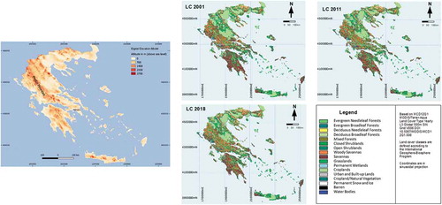
Figure 1. Aster GDEM (left side) and land cover types distribution in Greece in 2001, 2011 and 2018

According to the Hellenic Statistical Authority (2020) the country is oriented toward economy of services with the prevailing sector being the tourism. Industrial activities and agriculture production also contribute, to a lower extent to economic growth. Since 2010 the country has experienced a dramatic economic recession, with raise in unemployment, massive business closures and abrupt collapse of private sector, increasing poverty and homelessness, and a fall in consumer’s spending on goods and services (Tsampra 2018), accompanied by a drop in investments in industry and urban expansion (Cecchini et al. 2018) but also a serious decline in country’s population of approximately 2%. According to Labrianidis and Pratsinakis (2014), 210.184 people left Greece in the five-year period of 2010 to 2014 and approximately another 12.500 people followed them in the first trimester of 2015.

According to the latest, i.e. 2018, MODIS land cover image based on the International Geosphere-Biosphere Program (IGBP) classification, the major part of the country is occupied by dense and sparse forests (Deciduous and Evergreen Forests, Mixed Forests, Savannas, Woody Savannas) occupying ~52% of the country’s area, followed by Grasslands ~22%, and Croplands ~20%. (Figure 1) shows the Digital Elevation Model of Greece (ASTER GDEM) (NASA/METI/AIST/Japan Space Systems 2018) and the distribution of land cover types in Greece on 2001, 2011, and 2018.

2.2 Description of the data set

The dominant historical land cover transitions were identified from 2001, 2011 and 2018 land cover images from the annual MODIS MCD12Q1v006 product (Sulla-Menashe and Friedl 2019), at a spatial resolution of 500 m. The MODIS land cover is produced with supervised classification using the MODIS reflectance data to acquire land cover images (Strahler et al. 1999). Although the spatial resolution of 500 m is restrictive for use at the local scale, it is suitable to capture land cover transitions at the regional scale and various previous works have used MODIS land cover products for regional and local assessments (Sharma et al. 2017; Vijith and Dodge-Wan 2020; H. Yang et al. 2020; Demattê et al. 2020). The Collection 6 of the MODIS MCD12Q1 has been validated at stage 2, i.e. it has undergone extensive validation using ground-truth tests, under several time periods and in numerous locations widely distributed around the globe (Sulla-Menashe and Friedl 2019). The overall product accuracy has been reported to 73.6% (Sulla-Menashe et al. 2019). MODIS land cover are Level 3 products. Improvements in Collection 6 are related to improved quality of lower level input data sets such as cloud screening, atmospheric correction, and surface reflectance, which provided an improved context for land cover mapping. The algorithm for global land cover mapping used in Collection 6 MODIS land cover, is based on a hierarchical classification model. As described in Sulla-Menashe et al. (2019) the classes included in each level of the hierarchy reflect structured distinctions between land cover properties. An important improvement of Collection 6 compared to Collection 5 is the reduction of spurious land cover changes introduced by classification uncertainty in individual years. This was achieved by applying a hidden Markov model. Eight classification schemes are included in the Collection 6 of the MODS land cover product, with the most detailed provided by the classification of the International Geosphere-Biosphere Program (IGBP), categorizing Earth’s surface into 17 distinct categories. This specific categorization scheme was adopted in the present work. Known issues of the product are reported in Sulla-Menashe et al. (2019). Those are related to the underestimation of Cropland areas in the tropics, the misclassification of Evergreen Needleleaf Forests as Broadleaf Evergreen Forests in the temperate zones, but also the classification of Grasslands as Savannas. Problems are also reported in the determination of areas covered with permanent sea ice and glaciers. An evaluation exercise of the MODIS land cover product was present by Liang et al. (2015), intercomparing the MODIS land cover with a fine resolution land cover data set, namely, Globeland30 at 30 m spatial resolution. Therein authors concluded that there is a strong consistency of area percentage, spatial consistency, classification accuracy, and landscape diversity of MCD12Q1 based on GlobeLand30. Additionally, among the various MODIS land cover classification schemes, IGBP shows the best compatibility and robustness, indicating that the consistency of IGBP is the best at the regional scale (Liang et al. 2015). The MCD12Q1 IGBP classification has also been used as reference layer to define training class labels and classify Landsat images to generate 30 m land cover maps (Zhang and Roy 2017). In the present work to test the potential of the MODIS IGBP classification to describe the landscape characteristics of the study area, the MODIS land cover 2018 was compared with a reference data set, i.e. CORINE land cover 2018 from the European land cover inventory, released at intervals of six years at a spatial resolution of 100 m (European Union 2018). CORINE land cover was resampled with the nearest-neighbor interpolation, which is an appropriate method to resample categorical data (Liang et al. 2015) to match the MODIS land cover spatial resolution. As the land cover classes in the two datasets are quite different, a harmonization was achieved reclassifying the MODIS IGBP layer into the five major CORINE land cover classes (Label 1 in the CORINE land cover legend), i.e. Artificial surfaces, Agricultural areas, Forest and Semi-natural areas, Wetlands, Water bodies. Then, the similarity metrics of the MODIS and CORINE land cover were evaluated.

The ASTER Global Digital Elevation Model (GDEM) Version 3 (NASA, METI, and AIST 2019) at spatial resolution of approximately 30 m (resampled using a bilinear interpolation to match the MODIS land cover product) was also used as a Driver Variable for land cover transitions (Figure 1).

Historical and future climate data from the WorldClim platform were accessed (https://www.worldclim.org/data/index.html, last accessed on 10 November 2020). Historical monthly data from 2000 to 2018 were acquired in the form of mean minimum temperature (°C), mean maximum temperature (°C) and total precipitation (mm) at 2.5 minutes grids (Harris et al. 2014). Monthly temperature data were averaged over the whole period to extract the mean annual minimum and maximum temperature, respectively. Annual precipitation was computed from monthly values. The mean annual precipitation was computed for the whole period, i.e. from 2000 to 2018. Those variables were assessed for their degree of association with the distribution of land cover categories and those found to have a good predictive power were introduced in the model.

Future scenarios for the same climatic variables are available from WorldClim platform at 20-year intervals up to 2100, based on the Coupled Model Intercomparison Project 6 (CMIP6). Four Shared Socio-economic Pathways (SSPs) are available: SSP126, SSP245, SSP370, and SSP585. SSPs are analogous to the IPCC’s AR5 Representative Concentration Pathways (RCPs) which describe different possible greenhouse gas emissions. In CMIP6 the four RCPs, i.e. RCP2.6, RCP4.5, RCP6.0, and RCP8.5 are represented by the four SSPs, i.e. SSP126, SSP245, SSP360, and SSP585, respectively, in the sense that they result in similar 2100 radiative forcing as the specific RCPs. CMIP6 has one more SSP, i.e the SSP370 which describes the middle of the road” scenario. SSPs also describe how socioeconomic factors such as population, economic growth, education, urbanization, and the rate of technological development may change over the next century. In the present work, two future scenarios were examined, i.e., SSP126 and SSP585 for the 2021–2040. SSP126 corresponds to the optimistic case representing the sustainability route. SSP585 refers to worst case of fossil-fueled development. WorldClim provides monthly averages at 2.5 minutes spatial resolution for the whole twenty-year period, while for the needs of the present work mean annual values were computed, assuming that they are representative of the prediction period, i.e. 2018–2030. WorldClim provides future climate from CMIP6 based on eight GCMs (Harris et al. 2014; L. Feng et al. 2020). In the present work an ensemble of 4 GCMs was used, i.e., BCC-CSM2-MR, CNRM-ESM2-1, PSL-CM6A-LR and MIROC-ES2L. To match the spatial resolution of MODIS land cover data, the gridded climate variables were resampled with a bilinear interpolation.

Future scenarios, as expressed by the SSPs, incorporate the economic development aspects and they were used herein to examine impacts of economic growth on land cover changes and acquire predictions based on various socioeconomic narratives.

2.3 Analysis of historical observations

Developing an LCM requires the study of historical land cover transitions and evaluation of their potential origin. As the land cover classification used herein comprises 17 classes, the potential combination of land cover transitions is very large and cannot be accommodated by a single model. To address this problem and model only those transitions that impact landscape to a substantial degree, the dominant land cover transitions were determined, and they were grouped into a single sub-model. It is important to keep in mind that not all transitions can be grouped in a single sub-model, as their origin might be quite different, e.g. urban expansion with afforestation would be quite difficult to be modeled under a single sub-model. Therefore, land cover transitions in two periods, i.e. from 2001 to 2011 and from 2011 to 2018 were evaluated. In this work land cover transitions corresponding to net changes ≥1.5% of the country in both periods were regarded as dominant and were incorporated in the LCM.

2.4 Land change model

2.4.1 Model development

The modeling process for simulating land transitions in Greece was that described in Eastman (2016). All computations, i.e. the land cover image analysis as well as the training, testing, and verification of LCM was conducted within the Land Change Modeler incorporated in Terrset: Geospatial Monitoring and Modeling System (Eastman 2016). After deciding on the transitions to be modeled, a collection of transitions potential maps is introduced in the transition sub-model, assumed to have the same driver variables. Those are used to model the transition process in the past. Various models can be applied to simulate the transitions of land, such as machine learning techniques which can handle highly nonlinear problems, like the Multi-Layer Perceptron (MLP) or the Similarity Weighted Instance-based Learning (Sangermano and Eastman 2010) or even logistic regression, but only MLP can group and model multiple transitions with a single sub-model (Eastman, Solorzano, and Van Fossen 2005). Next, Driver Variables (also known as explanatory or predictor variables) are identified and their predictive ability in the model is evaluated. Those can be either specified as static or dynamic, i.e. changing over time. There is also the possibility to incorporate restrictions or incentives in the form of zoning maps or land development areas. In the present LCM, due to the nature of historical dominant changes of transitions to more natural landscape types, six variables were examined, a) the Evidence Likelihood of Land Cover which is the relative frequency of pixels of different land cover classes within the areas of change, b) Altitude (from the ASTER GDEM), c) Distance from previously changed land, d) Mean Annual Minimum Temperature (2000–2018), e) Mean Annual Maximum Temperature (2000–2018) and f) Mean Annual Precipitation (2000–2018). The predictive ability for each of those variables was tested using the Cramer’s V quantitative measure of association, which is an indicator of the potential but not guaranteed explanatory value of a variable. Cramer’s V indicates the degree to which the variable is associated with the distribution of land cover categories and according to Eastman (2016) a Cramer’s V around 0.15 or higher may be useful, whereas those with Cramer’s V ≥ 0.4 are potential good predictors. The p-value, i.e. the probability that the Cramer’s V is not significantly different from zero, is also examined at this stage.

Following, the MLP takes the Driver Variables found to have good predictive ability and introduces them in the computational process to produce the transition potential or suitability of change maps. A large random sample of pixels belonging to two categories, i.e. those that changed and those that persisted is automatically taken and half of it is used for training the network while the rest half is used for testing its performance. The network architecture is determined automatically but parameters such as number of hidden layer nodes, momentum factor, and sigmoid constant a, start and end learning rates can be altered by the user to achieve better outcome. The learning procedure is dynamic and starts with an initial value of learning rate which reduces progressively. Learning rates (start and end) are also reduced in cases when large oscillations in the RMS error are observed (Eastman 2016). The accuracy and skill (the measured accuracy minus the accuracy expected by change) of the model are then reported along with a breakdown of skill to the involved transitions and persistences. Once a good performance is reached either as low RMS error (<0.01) or a high accuracy rate (>80%), then the model is considered reliable to be used for future predictions. In the present work the MLP was trained and tested using the predefined Driver Variables and the 2001 and 2011 MODIS land cover images as start and end dates for model development.

2.4.2 Model verification and application for future prediction

After the LCM was developed, it was applied for a new end date, which in the present work was chosen to be the 2018 (last available MODIS land cover image at the time of completion of the present work). The same dominant land cover transitions as in the past were used for the 2018 prediction. Markov Chain analysis provided a transition probability matrix that quantifies change in each transition. The LCM was then verified by comparing the predicted land cover image for 2018 to the observed one. Classification metrics were computed from the error matrix. Therefore, the classification accuracy was assessed by the Producer’s Accuracy (PA), i.e. the area in each land cover type classified accurately divided by the total area of that class, User’s Accuracy (UA), i.e. the total area correctly classified for a specific class divided by the row total in the error matrix, and the Overall Accuracy (OA), calculated adding the correctly classified areas and dividing it by the total area of study. The Kappa Coefficient (K), ranging from −1 to 1, is also used to evaluate the accuracy of the classification presented in two images, which describes how well the model performed compared to random value assignment. K is known as the interrater variability, and describes the level of random agreement between data collectors when they do not know the correct answer but they are mostly guessing (Mchugh 2012; Cohen 1960). When $K$ values are close to 1 they indicate significantly better classification than random. Kappa Coefficient is computed from the following formula:

(1) $K=(P_o-P_e)/\left(1-P_o\right)$(1)

where $P_e$ is the probability of random agreement and $P_o$ is the probability of agreement. When two classification images are compared, $K$ is calculated based on the following formula:

(2) $K=\frac{N{\sum }_{i=1}^n{m}_{i,i}-{\sum }_{i=1}^n(G_i{C}_i)}{N^2-{\sum }_{i=1}^n(G_i{C}_i)}$(2)

where i is the number of classes, N is the total number of classified values compared to truth values, $m_{i,i}$is the number of correctly classified instances, $C_i$ is the number of instances precited of class i, $G_i$are true number of instances of class i.

The verified model was then applied to predict the land cover for Greece in 2030 under two SSPs, i.e. the SSP126 (sustainable development) and the SSP585 (worst case scenario).

3. Results and discussion

Results of the comparison of MODIS land cover 2018 with the CORINE land cover 2018 (reference data set) provided an overall accuracy of MODIS land cover IGBP of 82.3%. The User’s and Producer’s accuracy along with the K coefficient for individual classes can be found in Supplementary Material S1. Thus, it seems that MODIS depicts the major landscape characteristics of the study area.

Analysis of historical MODIS land cover data for 2011, 2011, and 2018 revealed that four are the dominant transitions (those with net changes ≥1.5% of country’s area) in both examined periods: Grasslands to Savannas, Savannas to Woody Savannas, Savannas to Grasslands, and Croplands to Grasslands as highlighted in (Figure 2, Figure 3 and Table 1). The spatial distribution of dominant changes shown in (Figure 2), indicates that the west part of Greece was dominated primarily by Savannas to Woody Savannas transitions, whereas the rest of the country experienced all kinds of transitions in both examined periods.

Figure 2. Spatial distribution of dominant land cover changes in Greece from 2001 to 2011 and from 2011 to 2018, based on MODIS land cover product and the International Geosphere-Biosphere Program classification scheme. Coordinates are in MODIS sinusoidal projection

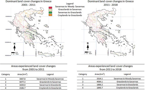
Figure 3. Gains and losses of various land cover types in Greece from 2001 to 2011 and from 2011 to 2018

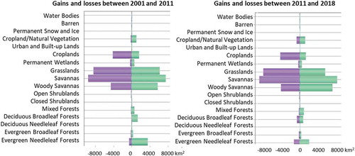
Table 1. Areas of various land cover types in Greece, in 2001, 2011, and 2018, based on MODIS land cover product

Land Cover type	2001		2011		2018
	Area (km^2)	Area (%)	Area (km^2)	Area (%)	Area (km^2)	Area (%)
Evergreen Needleleaf Forests	5396.7	4.08	8302.1	6.27	8938.8	6.75
Evergreen Broadleaf Forests	937.6	0.71	1084.0	0.82	1195.4	0.90
Deciduous Needleleaf Forests	0.5	0.00	0.0	0.00	1.7	0.00
Deciduous Broadleaf Forests	3194.8	2.41	4379.0	3.31	4572.9	3.45
Mixed Forests	2001.9	1.51	2514.5	1.90	3084.0	2.33
Closed Shrublands	30.5	0.02	26.2	0.02	13.7	0.01
Open Shrublands	299.0	0.23	188.7	0.14	211.0	0.16
Woody Savannas	15,889.9	12.00	17,053.1	12.88	19,330.2	14.60
Savannas	34,632.4	26.15	32,556.0	24.58	32,074.9	24.22
Grasslands	32,830.8	24.79	30,574.0	23.09	28,829.7	21.77
Permanent Wetlands	2033.9	1.54	2265.9	1.71	2452.7	1.85
Croplands	31,112.0	23.49	28,580.1	21.58	26,461.6	19.98
Urban and Built-up Lands	2044.6	1.54	2055.6	1.55	2066.3	1.56
Cropland/Natural Vegetation Mosaics	808.0	0.61	1650.7	1.25	1985.6	1.50
Permanent Snow and Ice	0.9	0.00	0.5	0.00	0.5	0.00
Barren	319.6	0.24	244.3	0.18	266.6	0.20
Water Bodies	901.6	0.68	959.7	0.72	948.8	0.72
Total	132,434.6	100	132,434.6	100.0	132,434.6	100.0

From the types of dominant transitions, (Grasslands to Savannas, Savannas to Woody Savannas, Savannas to Grasslands and Croplands to Grasslands) it seems that the landscape is in general transforming into more natural types of land cover and it was assumed that the origin of those transitions was mostly land abandonment due to economic crisis and population leaving abroad. Additionally, the Urban and Built-up lands which correspond to human-impacted areas, remain almost unchanged, whereas Barren land which is expected to have been increased in an area experiencing desertification or land degradation impacts also demonstrates no changes, as evidenced by the information in (Table 1). Furthermore, Croplands have experienced substantial losses in both examined periods (Table 1). It is, therefore, reasonable to conclude that all four transitions have the same origin and thus they may be modeled under a single sub-model.

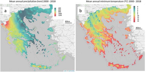
The next step is to identify potential Driver Variables and therefore the Cramer’s V values were examined for Evidence Likelihood of Land Cover, Altitude, Distance from previous changes, Mean Annual Minimum Temperature, Mean Annual Maximum Temperature and Mean Annual Precipitation and it was found to be 0.3592 for Evidence Likelihood of Land Cover, 0.1836 for Altitude, 0.1821 for Mean Annual Precipitation, 0.1718 for Mean Annual Minimum Temperature, 0.1546 for Distance from previous changes, and 0.1312 for Mean Annual Maximum Temperature, with p < 0.01 for all variables. Therefore, the five predictor variables with Cramer’s V values > 0.15 were incorporated in the LCM, whereas Mean Annual Maximum Temperature was excluded. (Figure 4) shows the two climatic variables introduced in the model. Due to the dynamic character of the Evidence Likelihood of Land Cover and Distance from previous changes parameters, those two variables were incorporated in the model as dynamic variables and were recalculated at each specified time step, which for the present work was selected to be one year. Climatic variables were evaluated as static throughout the 2001 to 2018 period.

Figure 4. Historical climate data from 2000 to 2018 at 2.5 minutes grids (Harris et al. 2014): a) Mean Annual Precipitation (mm) and b) Mean Annual Minimum Temperature (^oC)

The starting and ending year for LCM development was 2001 and 2011, respectively. The random sample created for the model training and testing was set to 10,000 pixels (half of it used for training and half for testing), thus the MLP was fed with cases from seven classes (four transition classes and three persistent classes, i.e. those participating in the dominant land cover transitions). The size of the training and testing datasets are set based on the minimum number of pixels that transitioned among the dominant land cover transition types. The MLP creates then a network of neurons that connects the five input variables from the Driver Variables and the seven output classes (the transition and persistence classes). A set of random initial weights, i.e. the multivariate function, are applied to the network and the error in the training data is computed and adjusted within each iteration. The model parameters in the LCM development phase are changed many times, until a satisfactory model performance is achieved.

The network architecture and parameterization as well as performance metrics are shown in (Table 2). The model skill breakdown by transition and persistence is shown in (Table 3).

Table 2. Multilayer Perceptron LCM parameters

Independent Variable 1	Evidence Likelihood of Land Cover
Independent Variable 2	Altitude (ASTER GDEM)
Independent Variable 3	Mean Annual Precipitation
Independent Variable 4	Mean Annual Minimum Temperature
Independent Variable 5	Distance from previous changes
Number of pixels for training	5000
Number of pixels for testing	5000
Input layer neurons	5
Hidden layer neurons	7
Output layer neurons	7
Final learning rate	0.001
Momentum factor	0.5
Sigmoid constant	1
Acceptable RMS	0.01
Iterations	9343
Training RMS	0.0078
Testing RMS	0.0082
Accuracy rate	97.32%
Skill measure	0.8632

Table 3. LCM skill breakdown by transition and persistence

Class	Skill measure
Transition: Savannas to Woody Savannas	0.9579
Transition: Savannas to Grasslands	0.9588
Transition: Grasslands to Savannas	0.9691
Transition: Croplands to Grasslands	0.9508
Persistence: Savannas	0.7485
Persistence: Grasslands	0.7367
Persistence: Croplands	0.7212

Sensitivity of model to holding specific input variables constant is examined and the results are shown in (Figure 5). After the model was trained using all Driver Variables, the model performance was tested keeping one variable at a time constant at its mean value, removing thus variability associated with this specific variable.

Figure 5. LCM sensitivity analysis, a) forcing a single variable constant, b) forcing all variables except one to be constant, c) using backward stepwise constant forcing

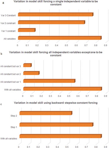
(Figure 5a) shows the result of forcing a single input variable to be constant to its mean value. It appears that holding variable 1 (Evidence Likelihood of Land Cover) constant has the most severe impact on the model. Model performance is moderately impacted keeping constant variable 2 (Altitude) and variable 3 (Mean Annual Precipitation), while keeping variable 4 (Mean Annual Minimum Temperature) and variable 5 (Distance from previous changes) constant has the least effect on LCM output. It seems thus that the most influential variable is Evidence Likelihood of Land Cover, having a strong effect on model performance, followed by Altitude and Mean Annual Precipitation.

(Figure 5b) demonstrates the case when all variables remain constant except one. The same outcome as in (Figure 5a) is extracted, with variable 1 being the most important, with the rest two exhibiting considerably less skill, but the combination of all five has the best skill result.

(Figure 5c) shows the case of first holding constant the variable with the least impact (step 1), then adds sequentially the next variable (step 2), such that the pair of variables held constant this time has the least effect on the LCM. The process continues until only one variable is left, helping thus on deciding on the LCM that explains most of the variability while using the least number of variables. The process is known as backward stepwise constant forcing and it helps on reducing number of variables, especially in LCMs with numerous Driver Variables, minimizing thus the overfitting possibility.

In the present LCM, although Evidence Likelihood of Land Cover seems to have the strongest predictive power, the other four variables also have positive effects on the model and it was thus decided to keep them all, since the number of Driver Variables is already small.

After the training and testing phase is completed and a satisfactory performance is achieved, the LCM is used to predict land cover for 2018, by constructing a Markov Chain table and computing the amount of expected change in each land cover category. The same Driver Variables are used this time as well, with Evidence Likelihood of Land Cover and Distance from previous changes, being dynamic, i.e. they are recalculated in each time step. LCM performance was assessed by comparing the predicted and observed 2018 land cover images. The Producer’s (PA) and User’s Accuracy (UA) together with the Overall Accuracy (OA) and K coefficient are shown on (Table 4).

Table 4. Classification accuracy of predicted versus observed 2018 land cover

	User’s Accuracy %	Producer’s Accuracy (%)	Overall Accuracy (%)	Kappa Coefficient
Evergreen Needleleaf Forests	81.7	94.8	96.7 (p < 0.01) 95% confidence interval: 96.51–96.72	0.959
Evergreen Broadleaf Forests	79.6	92.9
Deciduous Needleleaf Forests	76.2	99.6
Deciduous Broadleaf Forests	85.9	98.1
Mixed Forests	77.8	94.8
Closed Shrublands	27.8	26.5
Open Shrublands	66.3	97.3
Woody Savannas	99.8	92.1
Savannas	99.1	97.3
Grasslands	99.7	98.7
Permanent Wetlands	83.5	97.1
Croplands	99.8	99.1
Urban and Built-up Lands	99.5	99.8
Cropland/Natural Vegetation Mosaics	58.7	99.7
Permanent Snow and Ice	100	100
Barren	83.6	94.8
Water Bodies	98.9	97.8

The same procedure was followed to acquire prediction on land cover transitions for 2030, using the climate variables, i.e. Mean Annual Precipitation and Mean Annual Minimum Temperature for the period 2021 to 2040 as provided from the two SSPs (Figures 6 and 7). Basic statistics over the study area for the two climatic variables can be found in (Table 5). The classification outcome for 2018 and 2030 are shown in (Table 6) and in (Figures 8 and 9).

Figure 6. Future climate data (2021–2040) from CMIP6 at 2.5 minutes grids (Harris et al. 2014; L. Feng et al. 2020) provided as ensembles of 4 GCMs, i.e. BCC-CSM2-MR, CNRM-ESM2-1, PSL-CM6A-LR and MIROC-ES2L: a) Projected mean annual precipitation and b) mean annual minimum temperature based on the SSP126

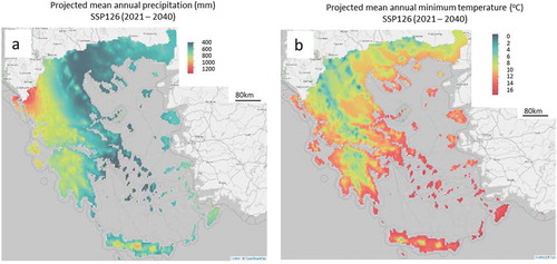
Figure 7. Future climate data (2021–2040) from CMIP6 at 2.5 minutes grids (Harris et al. 2014; L. Feng et al. 2020) provided as ensembles of 4 GCMs, i.e. BCC-CSM2-MR, CNRM-ESM2-1, PSL-CM6A-LR and MIROC-ES2L: a) Projected mean annual precipitation and b) mean annual minimum temperature based on the SSP585

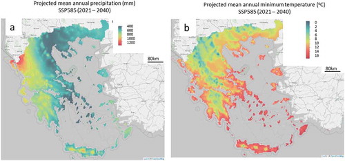
Figure 8. Comparison of observed land cover for 2001, 2011 and 2018, and predicted land cover for 2018 and 2030 in Greece under SSP126 and SSP585

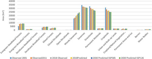
Figure 9. Spatial distribution of land cover transitions for the two examined scenarios, i.e. SSP126 and SSP585, for 2030 in Greece with reference the observed 2018 land cover

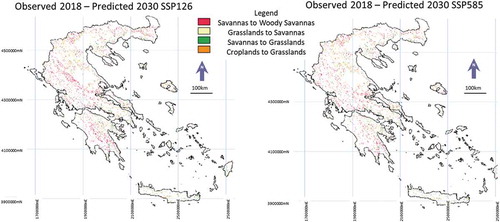
Table 5. Basic statistics of the examined climate scenarios over the study area

	Historical 2001–2018	SSP126 (2021–2040)*	SSP585 (2021–2040)*
Mean annual precipitation (mm/year)
Mean	681.2	653.6	643.3
Standard deviation	171.3	166.6	162.4
Minimum	392.3	391	381.7
Maximum	1389.1	1238	1211.9
Mean annual minimum temperature (°C)
Mean	9.8	10.6	10.7
Standard deviation	2.9	2.8	2.7
Minimum	−0.7	3.4	3.6
Maximum	17.5	17.7	17.8

*Averages of four GCMs: BCC-CSM2-MR, CNRM-ESM2-1, PSL-CM6A-LR, and MIROC-ES2L

Table 6. Predicted versus observed land cover areas in various land cover types for 2018 and predicted land cover for 2030 under SSP126 and SSP585

Land Cover type	2018 Observed		2018 Predicted		2030 Predicted SSP126			2030 Predicted SSP585
	Area (km^2)	Area (%)	Area (km^2)	Area (%)	Area (km^2)	Area (%)	% change from observed 2018	Area (km^2)	Area (%)	% change from observed 2018
Evergreen Needleleaf Forests	8938.8	6.75	8635.2	6.52	8978.6	6.78	0.03	9028.1	6.82	0.07
Evergreen Broadleaf Forests	1195.4	0.90	1117.2	0.84	1221.9	0.92	0.02	1285.6	0.97	0.07
Deciduous Needleleaf Forests	1.7	0.00	2.0	0.00	0.0	0.00	0.00	0.0	0.00	0.00
Deciduous Broadleaf Forests	4572.9	3.45	4213.9	3.18	4587.5	3.46	0.01	4597.3	3.47	0.02
Mixed Forests	3084.0	2.33	2793.7	2.11	3121.1	2.36	0.03	3133.2	2.37	0.04
Closed Shrublands	13.7	0.01	15.4	0.01	16.5	0.01	0.00	16.9	0.01	0.00
Open Shrublands	211.0	0.16	162.5	0.12	197.8	0.15	−0.01	198.1	0.15	−0.01
Woody Savannas	19,330.2	14.60	21,014.5	15.87	24,282.8	18.34	3.74	22,997.4	17.37	2.77
Savannas	32,074.9	24.22	31,565.8	23.83	30,731.3	23.20	−1.01	30,986.0	23.40	−0.82
Grasslands	28,829.7	21.77	29,132.6	22.00	26,783.8	20.22	−1.54	27,357.2	20.66	−1.11
Permanent Wetlands	2452.7	1.85	2311.6	1.75	2436.8	1.84	−0.01	2438.0	1.84	−0.01
Croplands	26,461.6	19.98	26,991.2	20.38	24,853.0	18.77	−1.21	25,184.0	19.02	−0.96
Urban and Built-up Lands	2066.3	1.56	2057.2	1.55	2068.4	1.56	0.00	2068.3	1.56	0.00
Cropland/Natural Vegetation Mosaics	1985.6	1.50	1235.6	0.93	1916.7	1.45	−0.05	1925.2	1.45	−0.05
Permanent Snow and Ice	0.5	0.00	0.4	0.00	0.5	0.00	0.00	0.4	0.00	0.00
Barren	266.6	0.20	233.0	0.18	274.6	0.21	0.01	255.9	0.19	−0.01
Water Bodies	948.8	0.72	952.7	0.72	963.4	0.73	0.01	963.0	0.73	0.01
Total	132,434.6	100.0	132,434.6	100.0	132,434.6	100.0	0.0	132,434.6	100.0	0.0

From the above results, it is evident that the main change by the end of 2020–2030 decade according to both examined SSPs, is related to gains in the areas of Woody Savannas, which for the case of Greece correspond to sparse forest areas. The results of SSP126 demonstrate an accelerating expansion of Woody Savannas in the expense of Grasslands, Croplands, and Savannas. SSP585 resulted in a lower expansion rate of Woody Savannas and a decreased rate of losses for Savannas, Grasslands, and Croplands. It seems thus that the direction of historical changes will also prevail in the next decade, with the most severe scenario, i.e. SSP585 slowing down the rate of changes and the most sustainable one, i.e. SSP126, accelerating the rate of expansion of woody vegetation land cover type. A possible cause of those changes might be the decreased precipitation availability which might impact croplands, whereas woody vegetation seems to be more resilient to precipitation decrease. In any case the differences between the two examined scenarios for 2030 are not that pronounced, probably because climate variables are less impactful parameters in the present model compared to Evidence Likelihood of Land Cover parameter. Moreover, all other forest types are also gaining areas, indicating that the historical transitions will also continue in future as well. However, as far as the close future is concerned, there is no evidence that Greece will undergo a dramatic land cover transformation. even in the case of country’s return to rapid economic growth, after the long recession period during the last ten years, as long as climate and socioeconomic conditions are within the ranges of the two examined SSPs. Limitations of the methodology are related to the uncertainties in remotely sensed information but also to lower expected model performance in cases of future abrupt and unpredictable changes induced by either natural disasters or geopolitical instabilities. Such enormous changes were not present in the data set used for model development, with a consequent decreased capacity of the model to handle such events.

Results presented herein are consistent with the previously published works (Gemitzi, Banti, and Lakshmi 2019; Banti, Kiachidis, and Gemitzi 2019) where greening phenological patterns were identified for almost all land cover types in Greece, based on time series analysis of remotely sensed MODIS NDVI, indicating the transition to natural landscape and a reduction of human disturbances.

Finally, comparing findings of the present work with previous publications concerning land degradation risk in Mediterranean that reported major concerns for Greece, for ~42,000 km² corresponding to 34% of the country’s area (Prăvălie, Patriche, and Bandoc 2017) and the desertification risk of Greece with a 15% of country’s area categorized at critical state of desertification (Karamesouti, Panagos, and Kosmas 2018), results presented in the present work do not support such findings, neither in the historical observations nor in the predictions up to the end of the decade. This discrepancy is attributed to the fact that desertification and land degradation assessments are based on models where climate and vegetation data which may be quite different for those in the study period of the present work. However, as global environmental observations become available through the numerous satellite missions, it is important to take advantage of this valuable information and use it to update existing models to acquire realistic and useful forecasts.

4. Conclusions

Within the present work an LCM was developed, tested and validated for Greece. A CA Markov model was created, trained, and validated using historical land cover observations from 2001 to 2018. Driver Variables comprising climate and socioeconomic variables that were associated with observed changes were determined and incorporated in the model. After verifying the model’s predictive ability, it was applied to predict the land cover transitions for 2030 under two different SSPs, i.e. SSP126 corresponding to a sustainable development and SSP585 corresponding to the worst-case scenario. Results indicated that four dominant transformations prevail in Greece during the last 20 years, i.e. transformation from Savannas to Woody Savannas and from Savannas to Grasslands, from Grasslands to Savannas, and from Croplands to Grasslands. The developed LCM demonstrated a satisfactory performance in all examined metrics. Those transitions seem to persist up to 2030 based on model’s predictions for both examined scenarios, indicating that the country experiences a land transformation to more natural and less human-disturbed types. However, the historical period used to train the model is impacted by the economic recession that Greece has undergone, and future predictions might be quite different, in case of a very rapid economic growth or major natural or human-induced events. Nevertheless, as far as the present and near future of the country is concerned, the land cover evolution seems to follow a sustainable route.

Data availability

MCD12Q1 v006MODIS/Terra+Aqua Land Cover Type Yearly L3 Global 500 m SIN Grid

data are available at no cost from the following url: https://lpdaac.usgs.gov/products/mcd12q1v006//last visited 20 August 2020).

WorldClim climate data are available at no cost at the following url:

https://www.worldclim.org/data/index.html

Acknowledgements

Author acknowledges the Technical Chamber of Greece for its support through the project Coupled use of remotely sensed and in situ observations for assessment of environmental changes” (Project ID: 82430, - Democritus University of Thrace). Author would like to thank the anonymous reviewers for their time and effort to review and improve this work

Disclosure statement

Author declares no conflict of interest

Supplementary data

Supplemental data for this article can be accessed here.

Additional information

Funding

This work was supported by the Technical Chamber of Greece, Project ID: 82430, - Democritus University of Thrace.

References

- Aitkenhead, M. J., and I. H. Aalders. 2009. “Predicting Land Cover Using GIS, Bayesian and Evolutionary Algorithm Methods.” Journal of Environmental Management 90 (1): 236–250. doi:10.1016/j.jenvman.2007.09.010.
- Assaf, C., C. Adams, F. F. Ferreira, and F. Helena. 2021. “Land Use and Cover Modeling as A Tool for Analyzing Nature Conservation Policies – A Case Study of Juréia-Itatins.” Land Use Policy 100: 104895. November 2018. doi:10.1016/j.landusepol.2020.104895.
- Banti, M. Α., K. Kiachidis, and A. Gemitzi. 2019. “Estimation of Spatio-Temporal Vegetation Trends in Different Land Use Environments across Greece Use Environments across Greece.” Journal of Land Use Science 1–16. doi:10.1080/1747423X.2019.1614687.
- Cecchini, M., I. Zambon, A. Pontrandolfi, R. Turco, A. Colantoni, A. Mavrakis, and L. Salvati. 2018. “Urban Sprawl and the ‘Olive’ Landscape: Sustainable Land Management for ‘Crisis’ Cities.” GeoJournal 1–19. doi:10.1007/s10708-018-9848-5.
- Cohen, J. 1960. “A Coefficient of Agreement for Nominal Scales.” Educational and Psychological Measurement 20: 37–46. doi:10.1177/001316446002000104.
- Demattê, J. A. M., J. L. Safanelli, R. R. Poppiel, R. Rizzo, N. E. Quiñonez Silvero, W. de Sousa Mendes, B. Roberto Bonfatti, et al. 2020. “Bare Earth’s Surface Spectra as a Proxy for Soil Resource Monitoring.” Scientific Reports 10 (1): 1–11. doi:10.1038/s41598-020-61408-1.
- Eastman, J. R. 2016. “Terrset: Geospatial Monitoring and Modeling System Manual.” Clask Labs, 1 – 393. Clark University (www.clarklabs.org).
- Eastman, J. R., L. A. Solorzano, and M. E. Van Fossen. 2005. “Transition Potential Modeling for Land-Cover Change.” In GIS, Spatial Analysis, and Modeling, edited by D. J. Maguire, M. Batty, and M. F. Goodchild, 357–385. Redlands: ESRI Press.
- Eleftheriou, D., K. Kiachidis, G. Kalmintzis, A. Kalea, C. Bantasis, P. Koumadoraki, M. E. Spathara, A. Tsolaki, M. I. Tzampazidou, and A. Gemitzi. 2018. “Determination of Annual and Seasonal Daytime and Nighttime Trends of MODIS LST over Greece - Climate Change Implications.” Science of the Total Environment 616–617: 937–947. doi:10.1016/j.scitotenv.2017.10.226.
- European Union. 2018. “Copernicus Land Monitoring Service 2018, European Environment Agency (EEA).” Corine Land Cover (CLC) 2018, Version 2020_20u1.” 2018. https://land.copernicus.eu/pan-european/corine-land-cover/clc2018
- Fallah Shamsi, S. R. 2010. “Integrating Linear Programming and Analytical Hierarchical Processing in Raster-GIS to Optimize Land Use Pattern at Watershed Level.” Journal of Applied Sciences and Environmental Management 14: 2. doi:10.4314/jasem.v14i2.57868.
- Feng, L., S. J. Smith, C. Braun, M. Crippa, M. J. Gidden, R. Hoesly, Z. Klimont, M. van Marle, M. van den Berg, and G. R. van der Werf. 2020. “The Generation of Gridded Emissions Data for CMIP6.” Geoscientific Model Development 13: 461–482. doi:10.5194/gmd-13-461-2020.
- Feng, Y., and X. Tong. 2018. “Dynamic Land Use Change Simulation Using Cellular Automata with Spatially Nonstationary Transition Rules.” GIScience and Remote Sensing 55 (5): 678–698. doi:10.1080/15481603.2018.1426262.
- Fernandes, M. M., M. Rodrigues de Moura Fernandes, J. Ruiz Garcia, E. A. Trondoli Matricardi, A. Quintão de Almeida, A. Siqueira Pinto, R. Simões Cezar Menezes, A. de Jesus Silva, and A. Herculano de Souza Lima. 2020. “Assessment of Land Use and Land Cover Changes and Valuation of Carbon Stocks in the Sergipe Semiarid Region, Brazil: 1992–2030.” Land Use Policy 99: 104795. doi:10.1016/j.landusepol.2020.104795. May.
- Gemitzi, A., M. Α. Banti, and V. Lakshmi. 2019. “Vegetation Greening Trends in Different Land Use Types : Natural Variability versus Human-Induced Impacts in Greece.” Environmental Earth Sciences 78 (5): 1–10. doi:10.1007/s12665-019-8180-9.
- Giorgi, F. 2006. “Climate Change Hot-Spots.” Geophysical Research Letters 33 (8): L08707. doi:10.1029/2006GL025734.
- Giorgi, F., and P. Lionello. 2008. “Climate Change Projections for the Mediterranean Region.” Global and Planetary Change 63 (2–3): 90–104. doi:10.1016/j.gloplacha.2007.09.005.
- Harris, I., P. D. Jones, T. J. Osborn, and D. H. Lister. 2014. “Updated High-Resolution Grids of Monthly Climatic Observations - the CRU TS3.10 Dataset.” International Journal of Climatology 34 (3): 623–642. doi:10.1002/joc.3711.
- Hellenic Statistical Authority. 2020. “The Greek Economy. Hellenic Republic Hellenic Statistical Authority.”
- Hereher, M. E. 2017. “Effects of Land Use/Cover Change on Regional Land Surface Temperatures: Severe Warming from Drying Toshka Lakes, the Western Desert of Egypt.” Natural Hazards 1–15. doi:10.1007/s11069-017-2946-8.
- Hyandye, C. 2015. “GIS and Logit Regression Model Applications in Land Use/Land Cover Change and Distribution in Usangu Catchment.” American Journal of Remote Sensing 3 (1): 6. doi:10.11648/j.ajrs.20150301.12.
- Hyandye, C., and L. W. Martz. 2017. “A Markovian and Cellular Automata Land-Use Change Predictive Model of the Usangu Catchment.” International Journal of Remote Sensing 38 (1): 64–81. doi:10.1080/01431161.2016.1259675.
- Karamesouti, M., P. Panagos, and C. Kosmas. 2018. “Model-Based Spatio-Temporal Analysis of Land Desertification Risk in Greece.” Catena 167: 266–275. March 2017. doi:10.1016/j.catena.2018.04.042.
- Labrianidis, L., and M. Pratsinakis. 2014. “Outward Migration from Greece during the Crisis.” Project Funded by the National Bank of Greece through the London School of Economic ’ s, https://www.lse.ac.uk/Hellenic-Observatory/Assets/Documents/Research/External-Research-Projects/Final-Report-Outward-migration-from-Greece-during-the-crisis-revised-on-1-6-2016.pdf
- Liang, D., Y. Zuo, L. Huang, J. Zhao, L. Teng, and F. Yang. 2015. “Evaluation of the Consistency of MODIS Land Cover Product (MCD12Q1) Based on Chinese 30 M GlobeLand30 Datasets: A Case Study in Anhui Province, China.” ISPRS International Journal of Geo-Information 4 (4): 2519–2541. doi:10.3390/ijgi4042519.
- Liping, C., S. Yujun, and S. Saeed. 2018. “Monitoring and Predicting Land Use and Land Cover Changes Using Remote Sensing and GIS Techniques—A Case Study of a Hilly Area, Jiangle, China.” PLoS ONE 13 (7): 1–23. doi:10.1371/journal.pone.0200493.
- Mchenry, M. P., S. N. Kulshreshtha, and S. Lac. 2015. “Land Use, Land-Use Change and Forestry.” Land Use, Land-Use Change and Forestry. doi:10.4337/9781849805834.00023.
- Mchugh, M. L. 2012. “Lessons in Biostatistics Interrater Reliability : The Kappa Statistic.” Biochemia Medica 22 (3): 276–282. doi:10.11613/BM.2012.031.
- NASA, METI, and AIST. 2019. “Japan Spacesystems, and U.S./Japan ASTER Science Team.” ASTER Global Digital Elevation Model V003 [Data Set]. NASA EOSDIS Land Processes DAAC, Accessed 30 July 2020. Https://Doi.Org/10.5067/ASTER/ASTGTM.003
- NASA/METI/AIST/Japan Space Systems, and U.S./Japan ASTER Science Team. 2018. “ASTER Global Digital Elevation Model V003, 2018, Distributed by NASA EOSDIS Land Processes DAAC.” Https://Doi.Org/10.5067/ASTER/ASTGTM
- Pnevmatikos, J. D., and B. D. Katsoulis. 2006. “The Changing Rainfall Regime in Greece and Its Impact on Climatological Means.” Meteorological Applications 13: 331–345. doi:10.1017/S1350482706002350.
- Prăvălie, R., C. Patriche, and G. Bandoc. 2017. “Quantification of Land Degradation Sensitivity Areas in Southern and Central Southeastern Europe. New Results Based on Improving DISMED Methodology with New Climate Data.” Catena 158 (February): 309–320. doi:10.1016/j.catena.2017.07.006.
- Ralha, C. G., C. G. Abreu, G. C. Cássio, A. Z. Coelho, B. Macchiavello, and R. B. Machado. 2013. “A Multi-Agent Model System for Land-Use Change Simulation.” Environmental Modelling and Software 42: 30–46. doi:10.1016/j.envsoft.2012.12.003.
- Sangermano, F., J. Ronald Eastman, and H. Zhu. 2010. “Similarity Weighted Instance-Based Learning for the Generation of Transition Potentials in Land Use Change Modeling.” Transactions in GIS 14 (5): 569–580. doi:10.1111/j.1467-9671.2010.01226.x.
- Sharma, R. C., K. Hara, H. Hirayama, I. Harada, D. Hasegawa, M. Tomita, J. G. Park, et al. 2017. “Production of Multi-Features Driven Nationwide Vegetation Physiognomic Map and Comparison to MODIS Land Cover Type Product.” Advances in Remote Sensing 06 (1): 54–65. doi:10.4236/ars.2017.61004.
- Shooshtari, J., T. S. Sharif, B. R. Namin, and K. Shayesteh. 2020. “Land Use and Cover Change Assessment and Dynamic Spatial Modeling in the Ghara-Su Basin, Northeastern Iran.” Journal of the Indian Society of Remote Sensing 48 (1): 81–95. doi:10.1007/s12524-019-01054-x.
- Singh, S. K., P. B. Laari, S. Mustak, P. K. Srivastava, and S. Szilárd. 2018. “Modelling of Land Use Land Cover Change Using Earth Observation Data-Sets of Tons River Basin, Madhya Pradesh, India.” Geocarto International 33 (11): 1202–1222. doi:10.1080/10106049.2017.1343390.
- Song, X. P., M. C. Hansen, S. V. Stehman, P. V. Potapov, A. Tyukavina, E. F. Vermote, and J. R. Townshend. 2018. “Global Land Change from 1982 to 2016.” Nature 560 (7720): 639–643. doi:10.1038/s41586-018-0411-9.
- Strahler, A., S. Gopal, E. Lambin, and A. Moody. 1999. “MODIS Land Cover Product Algorithm Theoretical Basis Document (ATBD) MODIS Land Cover and Land-Cover Change.” http://modis.gsfc.nasa.gov/data/atbd/atbd_mod12.pdf
- Subedi, P., K. Subedi, and B. Thapa. 2013. “Application of A Hybrid Cellular Automaton – Markov (Ca-markov) Model in Land-Use Change Prediction: A Case Study of Saddle Creek Drainage Basin, Florida.” Applied Ecology and Environmental Sciences 1 (6): 126–132. doi:10.12691/aees-1-6-5.
- Sulla-Menashe, D., and M. Friedl. 2019. “MCD12Q1 MODIS/Terra+Aqua Land Cover Type Yearly L3 Global 500m SIN Grid V006. 2019.” Distributed by NASA EOSDIS Land Processes DAAC, Accessed 29 July 2020. Https://Doi.Org/10.5067/MODIS/MCD12Q1.006
- Sulla-Menashe, D., J. M. Gray, S. P. Abercrombie, and M. A. Friedl. 2019. “Hierarchical Mapping of Annual Global Land Cover 2001 to Present: The MODIS Collection 6 Land Cover Product.” Remote Sensing of Environment 222: 183–194. April 2018. doi:10.1016/j.rse.2018.12.013.
- Tsampra, M. 2018. “Crisis and Austerity in Action: Greece.” In The New Oxford Handbook of Economic Geography, Edited by Gordon L. Clark, Maryann P. Feldman, Meric S. Gertler, and Dariusz Wójcik, 113–140. Oxford University Press. doi:10.1093/oxfordhb/9780198755609.013.39.
- Vijith, H., and D. Dodge-Wan. 2020. “Applicability of MODIS Land Cover and Enhanced Vegetation Index (EVI) for the Assessment of Spatial and Temporal Changes in Strength of Vegetation in Tropical Rainforest Region of Borneo.” Remote Sensing Applications: Society and Environment 18: 100311. doi:10.1016/j.rsase.2020.100311. March.
- Wijitkosum, S. 2016. “The Impact of Land Use and Spatial Changes on Desertification Risk in Degraded Areas in Thailand.” Sustainable Environment Research 26 (2): 84–92. doi:10.1016/j.serj.2015.11.004.
- Wirt, Bradford. 2020. “The African Sahel in Transition 2020.” https://lpdaac.usgs.gov/resources/data-action/african-sahel-transition/
- Yang, H., J. Wang, W. Xiao, L. Fan, Y. Wang, and J. Jerker. 2020. “Relationship between Hydroclimatic Variables and Reservoir Wetland Landscape Pattern Indices: A Case Study of the Sanmenxia Reservoir Wetland on the Yellow River, China.” Journal of Earth System Science 129: 1. doi:10.1007/s12040-020-1347-7.
- Yang, X., X. Q. Zheng, and L. N. Lv. 2012. “A Spatiotemporal Model of Land Use Change Based on Ant Colony Optimization, Markov Chain and Cellular Automata.” Ecological Modelling 233: 11–19. doi:10.1016/j.ecolmodel.2012.03.011.
- Yin, J., Z. Yin, H. Zhong, X. Shiyuan, H. Xiaomeng, J. Wang, and W. Jianping. 2011. “Monitoring Urban Expansion and Land Use/Land Cover Changes of Shanghai Metropolitan Area during the Transitional Economy (1979-2009) in China.” Environmental Monitoring and Assessment 177 (1–4): 609–621. doi:10.1007/s10661-010-1660-8.
- Zhang, H. K., and D. P. Roy. 2017. “Using the 500 M MODIS Land Cover Product to Derive a Consistent Continental Scale 30 M Landsat Land Cover Classification.” Remote Sensing of Environment 197: 15–34. doi:10.1016/j.rse.2017.05.024.