The synergistic use of microwave coarse-scale measurements and two adopted high-resolution indices driven from long-term T-V scatter plot for fine-scale soil moisture estimation

ABSTRACT

In an attempt to retrieve soil moisture content (SMC) from remote sensing techniques, this article suggests and evaluates a developed approach that overcomes three of the most fundamental limitations of the temperature–vegetation (T-V) scatter plot method that are (1) low accuracy of the T-V scatter plot method in cases that the corresponding scatter plot and its wet and dry edges are not formed appropriately, (2) incompatibility of the T-V index maps in different days, and (3) inability to obtain the absolute SMC values from the T-V indices. The research consists of three main steps. In the first step, the measurements of eight global in situ SMC networks were applied to select the most appropriate and accurate microwave remote sensing mission among from Advanced Microwave Scanning Radiometer 2, Soil Moisture and Ocean Salinity, and Soil Moisture Active Passive. The results outlined the superiority of SMAP’s products in terms of RMSE and correlation coefficient (root mean square difference (RMSE) = 0.3–0.12 m³/m³ and R = 0.53–0.93). At the second step, the 1-year T-V scatter plot was formed and then, two adopted soil moisture indices, namely the annual soil moisture index (ASMI_HR) and daily soil moisture index (DSMI_HR), were extracted. The ASMI_HR was driven from the annual wet and dry edges and a novel concept called “co-moisture line” was introduced to obtain the DSMI_HR. In the third step of the proposed method, Disaggregation based on Physical and Theoretical scale Change was applied as the downscaling algorithm with a novelty to identify the parameter of partial derivative of microwave data relative to SMC indices using the relationship between ASMI_HR and coarse-scale SMAP pixels. Across four SMAP coarse-scale pixels located in the study area, the corresponding parameter was obtained with the average correlation coefficient 0.7. This step was followed by integrating DSMI_HR and SMAP products to provide absolute SMC values at intermediate spatial resolution. The proposed method was evaluated on the agricultural site of Soil Moisture Active Passive Validation Experiment 2016-Manitoba. The ultimate results of the proposed method in terms of absolute SMC values proved promising consistency with field measurements (R = 0.66 and no-bias RMSE = 0.06 m³/m³).

KEYWORDS:

• Soil moisture
• remote sensing
• temperature-vegetation scatter plot method
• microwave remote sensing
• DisPATCh

Introduction

Since the amount of soil moisture content (SMC) is believed to be one of the critical state variables in the water budget, energy cycle, and plant growth, timely access to accurate estimates of SMC and its spatial distribution is relevant to many applications and research topics (Zhu, Jia, and Lv 2017a; Chen et al. 2018; Ford and Quiring 2019).

Remote sensing techniques present great promising means of monitoring land surface SMC thanks to the accessibility of the satellite images, their acceptable spatial/temporal resolutions, and their low cost (Wang and Qu 2009; Rodríguez-fernández et al. 2019). An increasing number of studies have found that the so-called “trapezoid” or “triangle” method, which exploits the thermal and the optical remote sensing observations, is one of the promising approaches to estimate SMC by remote sensing technique (Liu and Yue 2018; Garcia et al. 2014; Przeździecki and Zawadzki 2020; Yang and Zhang 2019). Retrieval of SMC from the “trapezoid” or the “triangle” method is generally grounded in a unique relationship among the SMC, surface temperature, and vegetation (Peng et al. 2015; Zhang and Zhou 2016; Ghahremanloo, Mobasheri, and Amani 2019). The relation between remotely sensed surface temperature and vegetation content has been investigated by several authors (Carlson, Gillies, and Perry 1994; Carlson, Gillies, and Schmugge 1995; Nemani et al. 1993; Gillies, Kustas, and Humes 1997; Lambin and Ehrlich 1996). Briefly, land surface temperature derived from remote sensing images is a combination of soil temperature and vegetation temperature, which, themselves, are the consequences of soil evaporation and vegetation transpiration, respectively (Wang et al. 2018). Vegetation and soil surface temperature decrease as the vegetation intensity increases (Carlson, Gillies, and Schmugge 1995; Sandholt, Rasmussen, and Andersen 2002). Therefore, there is a negative relationship between soil temperature and vegetation fraction (Carlson, Gillies, and Schmugge 1995). The rate of the mentioned negative relationship behaves not the same in different SMC and intensifies in the dry soil condition (Carlson, Gillies, and Schmugge 1995; Sandholt, Rasmussen, and Andersen 2002). This claim is the basic of the temperature–vegetation (T-V) scatter plot theory. According to this theory, in a T-V scatter plot, the two-dimensional points (V, T), each of which represents a pixel of the remote sensing image, distribute in a triangular or trapezoidal feature space that is made up of two edges, called the wet and dry edges (Gillies, Kustas, and Humes 1997; Wang et al. 2001; Vani, Pavan Kumar, and Ravibabu 2019). The distances between each point and the mentioned edges have been argued as the SMC dependent parameters and applied to develop a variety of linear or non-linear SMC indices (Zhang and Zhou 2016; Wang et al. 2018; Vani, Pavan Kumar, and Ravibabu 2019; Ghahremanloo, Mobasheri, and Amani 2019).

Temperature Vegetation Dryness Index (TVDI), which is calculated based on the empirical interpretation of the T-V triangle scatter plot, is one of the most frequently applied indices for monitoring SMC at the drainage basin scale, regional scale, and national scale (Garcia et al. 2014; Liu et al. 2017; Mohseni and Mokhtarzade 2020). A detailed overview of T-V scatter plot methods and various indices extracted from them can be found in Zhang and Zhou (2016) and Petropoulos, Ireland, and Barrett (2015.

Despite the critical research efforts and recent advances, the T-V scatter plot method is still challenging. The most serious concerns that restrict its applicability in all regions are, perhaps, as follows:

1. Regarding the accuracy, the T-V technique is usually premised on the assumption that a definite wet edge and dry edge are extractable from the scatter plot (Zhu et al. 2017b; Petropoulos et al. 2009). An unexpected difficulty arises when there are insufficient pixels with the comprehensive temperature and vegetation conditions (e.g. bare soil, stressed vegetation, saturated soil, and healthy vegetation) to form reliable and correct edges (Yang and Zhang 2019).

2. Assuming that the dry and wet edges of T-V scatter plots are obtainable for all days with various temperatures and vegetation conditions, the SMC index maps extracted on different days have inconsistent scales and are not necessarily comparable. The underlying concept is that SMC indices of different days are extracted from various T-V scatter plots and thus, calculated using different edges that have no explicit physical relationship. This issue restricts the applicability of the T-V method in the long-term monitoring of the SMC (Saber et al. 2020; Mohseni and Mokhtarzade 2020).

3. After all, the indices derived from the T-V scatter plot are some dimensionless proxy of the SMC and are not the SMC values that are required in many applications. In the last few years, some empirical and semi-empirical relationships and algorithms have been proposed in the literature to convert T-V indices to the SMC values (Wang and Qu 2009; Petropoulos, Ireland, and Barrett 2015). These techniques, which usually require the field measurements of SMC and other environmental parameters, are bound to the specific region and time of calibration.

Over the past decade, there has been a dramatic increase in the number of studies that have focused on addressing the limitations of the T-V scatter plot method.

Zhang et al. (2008), after arguing that the apparent dry and wet edges of the T-V scatter plot are not formed correctly on many days, proposed a theoretical dry edge using the energy balance equation. Zhang et al. (2014) employed the theoretical limiting edges discussed by (Zhang et al. 2008) to estimate a new SMC index called Temperature Rising Rate Vegetation Dryness Index (TRRVDI). To calculate TRRVDI, the rate of land surface temperature in the mid-morning and the fractional vegetation cover are respectively set as the vertical and horizontal axis of T-V scatter plot. Sun et al. (2017) investigated and compared three methods discussed by Moran et al. (1994), Long, Singh, and Scanlon (2012), and Chen, Sun, and Li (2016) for detecting the theoretical dry and wet edges. Sun et al. (2017) found that although these three methods have the same behavior in estimating dry edges, there are great differences among the wet edges extracted from the corresponding methods. Detecting the theoretical boundary of T-V scatter plot requires ground-based measurements and ancillary data (i.e. wind speed, air temperature, solar radiation, vegetation height), which limit their operational applications in SMC measurement.

Tang, Li, and Tang (2010) demonstrated that the observed wet and dry edges can be reliable, where there are a large number of pixels reflecting a full range of soil surface wetness and fractional vegetation cover to form a true trapezoidal in the T-V scatter plot. This condition cannot be easily realized due to the fact that the study area is not necessarily covered by a comprehensive vegetation and temperature condition Mohseni and Mokhtarzade (2020). Many studies considered the study area and the extent of the input remote sensing images large enough to address this issue. However, since T-V scatter plot method is applicable on the assumption of uniform atmosphere conditions over the whole study area, the extent of the study domain has some influence on the performance of the T-V scatter plot method (Long, Singh, and Scanlon 2012).

Minacapilli et al. (2016), after arguing that the large study area contradicts the assumption of uniform atmosphere conditions over the study area, proposed a time-domain triangle method to address the limitation of identifying the wet and dry edges and estimate actual evapotranspiration. In their study, the Priestley–Taylor parameter of each pixel, which is a proxy of evapotranspiration, is estimated using a pixel-by-pixel T-V feature space established from long-term temperature and vegetation measurements. Inspired by them, Zhu, Jia, and Lv (2017a) developed the Modified Temperature Vegetation Dryness Index (MTVDI), which is proposed in their earlier work (Zhu et al. 2017b), using a time-domain solution method rather than the traditional spatial domain solution method. To this end, MTVDI was extracted from pixel-by-pixel T-V scatter plot, obtained by exploring the temporal domains over each single image pixel.

Mohseni and Mokhtarzade (2020) proposed a new long-term T-V scatter plot, in which normalized NDVI is set as the horizontal axis and three different temperature factors are suggested as the vertical axis. From their long-term T-V scatter plot, they also extracted a novel non-linear soil moisture index that defines the locus of co-moisture points in the scatter plot as unequal distance curves.

It must be noted that the indices derived from the time-domain T-V scatter plot are some dimensionless proxy of the SMC, which have to be converted to the absolute SMC values. Zhu, Jia, and Lv (2017a) exploited a linear fit method developed by Mallick, Bhattacharya, and Patel (2009) to convert MTVDI to the SMC values. Minacapilli et al. (2016) used Priestley–Taylor equation in (Monteith 1965) to convert φ values extracted from the time-domain T-V scatter plot to the regional evapotranspiration. It is obvious that all of these methods have in common the need for ground-based SMC measurements and some other ancillary data for estimating the empirical relationship between T-V indices and absolute SMC values. This issue limits their applications to monitoring SMC. On the other hand, they are empirical and semi-empirical approaches and are limited to the conditions in which they are justified and are not applicable to other study area.

Among all of these techniques, methods that co-exploit T-V scatter plot indices and passive MW earth observations (EOs) have received particular attention. Using these techniques, one can obtain SMC from EOs without the requirement of any auxiliary in situ data.

The underlying concept is that passive MW remote sensing technology can quantify the thermal emission from the soil surface, which is convertible to the accurate soil moisture (Sun et al. 2020; Colliander et al. 2017; El Hajj et al. 2018). This technology, however, suffers from one serious shortcoming in terms of its coarse resolution (several tens of kilometers) (Piles et al. 2011; Djamai et al. 2016). The developments of some disaggregation algorithms make it possible to resample and disaggregate the values of the coarse-scale MW-derived SMC products into some sub-pixel values using optical/thermal-derived soil moisture indices. There is a considerable amount of literature on the appropriateness of these indices to increase the spatial resolution of microwave soil moisture data (Fang et al. 2013; Peng et al. 2015; Kim et al. 2017; Neuhauser et al. 2019). The accuracy of those disaggregation algorithms depends directly on how accurately the optical/thermal soil moisture indices are defined.

In this study, we attempt to address the mentioned restrictions of the T-V methods and estimate accurate SMC values at an appropriate spatial and temporal resolution. More specifically, the purpose of this study is to devise a technique that yields SMC values at intermediate spatial resolution via the integration of microwave (MW), thermal, and optical remote sensing images. Using optical and thermal images, the paper applied the 1-year T-V scatter plot introduced and investigated by Mohseni and Mokhtarzade (2020) to address the first and second constraints of the T-V scatter plot method (mentioned above). In this new paper, a novel concept, referred to as the co-moisture line, is introduced as the locus of points with equal SMC value and then is applied to calculate the SMC indices.

In the next step, using incorporating the proposed SMC indices into passive MW observations, we obtain the amount of land surface soil moisture in units of m³/m³. Due to the different spatial resolution between optical/thermal-derived indices and passive microwave SMC data, this incorporation must be performed under the disaggregation algorithms. Therefore, this step is aimed at deriving a benefit from the high accuracy of passive MW SMC products (less than 0.04 m³/m³ over non-forested areas) and the appropriate spatial resolution of our proposed optical/thermal soil moisture indices to resample the MW-derived SMC and simultaneously, convert the proposed SMC indices to the absolute SMC values.

Details of the study area, in situ measurements, and applied remote sensing data are presented in the next section. After that, the approach proposed to retrieve the surface SMC values at intermediate spatial resolution is introduced. Then, the obtained results and their evaluation using ground truth samples, as well as some discussions are provided. Finally, the last section is dedicated to the conclusions.

Study site and data description

Study area

The core of the study area is the site of Soil Moisture Active Passive Validation Experiment 2016-Manitoba (SMAPVEX16-MB) located in Manitoba, Canada (97.76–98.1 W, 49.39–49.76 N) (Colliander et al. 2019). The SMAPVEX16-MB site, which is shifted east and south of the location of the SMAPVEX12, is almost a flat area (slope of 0–2%) (Mcnairn et al. 2015). Eighty percent of the study area is covered by agricultural field including soybean (29% of the study area), spring wheat (24%), canola (12%), corn (11%), and alfalfa (8%) (Bhuiyan et al. 2018).

SMAPVEX16-MB site contains 9 permanent stations of Real-time In situ Soil Monitoring for Agriculture (RISMA) network and 50 temporary stations, all of which are placed on agricultural fields and operated jointly by the Agriculture and Agri-Food Canada (AAFC) and NASA’s Soil Moisture Active Passive (SMAP) mission (Figure 1) (Bhuiyan et al. 2018; Colliander et al. 2019). Because SMAPVEX16_MB was developed after the SMAP grid was established, all of the corresponding stations are geographically distributed within one SMAP pixel (Colliander et al. 2019). These features, along with variations in the range of soil type and land cover, allow for a comprehensive and dependable assessment of soil moisture retrieval algorithms and disaggregation methods (Dey et al. 2019).

Figure 1. Color composite of a Landsat 8 image over the SMAPVEX16-MB field campaign area (Colliander et al. 2019). In total, 9 RISMA stations and 50 temporary agricultural fields are shown by green stars and red rectangles, respectively. The inset shows the arrangements of the 16 sample sites within two different fields

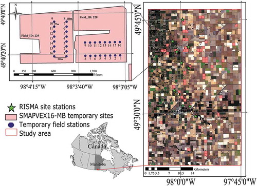
In each station of the RISMA network, three Stevens’ Hydra Probes are installed within the agricultural fields, about 6‐30 m away from the edge of them (Pacheco et al. 2014). Fifteen-minute and daily soil moisture and soil temperature measurements at the depth of 0–5, 5, 20, 50, and 100 cm are available in the RISMA data portal (http://aafc.fieldvision.ca/). On the other hand, in situ measurements of 50 temporary soil moisture stations were conducted over 12 weeks in 2016 (May 1 to August 31) (Bhuiyan et al. 2018). As the same strategy of SMAPVEX12 and CanEx-SM10, sampling points in each field are arranged every 75 m along two transects, which are separated by 200 m (Figure 1). Each sampling point hourly collects three measurements of surface SMC. Eventually, the average of the 48 measurements in each field is calculated and considered as the SMC of the corresponding field (~10 ha). Bhuiyan et al. (2018) briefly details the in situ measurement protocols. In this study, 0–5 cm SMC measurements are applied to validate the proposed method. Alongside soil moisture data, the air temperature measured at one of the RISMA station (station MB-5), which is approximately located in the center of our study area, was downloaded for the year 2016. The investigations of the air temperature measured by other RISMA stations shows that there is ±1.5° disagreement between the measurements of these stations. However, this uncertainty is less than the relative error of MODIS land surface temperature products (approximately 3°) and therefore is negligible.

Global soil moisture sites

Alongside the SMAPVEX16-MB in situ measurements, ground-based measurements from global SMC networks are applied as the reference data and validation sites to evaluate the SMC values derived from passive MW remote sensing satellites. Figure 2 represents the SRTM global elevation map and the location of the existent dense soil moisture sites – which include at least five stations – operated the National Aeronautics and Space Administration (NASA), natural resources conservation service (NRCS) agency of United States Department of Agriculture (USDA), and databases of the International Soil Moisture Network (ISMN) holding over 6100 soil moisture data sets of 1400 field stations operated by 40 different networks (Dorigo et al. 2015; Colliander et al. 2017).

Figure 2. SRTM global digital elevation map and location of the centers of the dense in situ validation sites. The selected sites are shown by red circles. Also, those sites that do not meet the time interval, station number, and geographic distribution criteria are illustrated by green, blue, and black circles, respectively

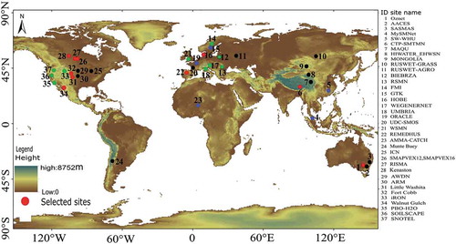
According to Jackson et al. (2010), among all of the sites shown in Figure 2, those that include at least eight stations (70% confidence for 0.03 m³/m³ soil moisture uncertainty with 0.07 m³/m³ variability) with invariant geographic distribution at a coarse-scale microwave pixel can be considered as the validation sites. Validation sites also should be employed over a relatively long time interval and located in the water-limited region, away from urban areas. Figure 2 specifies the sites that initially do not meet the time interval, station number, and geographic distribution criteria with green, blue, and black marks, respectively. Also, those sites that meet all the mentioned requirements are shown by red marks in Figure 2. These sites are applied as the validation sites in the first step of the proposed method. More detailed information about each selected site, such as the number of stations, the network area, and the performance duration, is represented in Section 4.1.

Space-based measurements

Passive microwave SMC products

Advanced Microwave Scanning Radiometer 2 (AMSR2) was launched on 18 May 2012 onboard the Global Change Observation Mission-1st Water (GCOM-W1) satellite by Japan Aerospace Exploration Agency (JAXA) to observe the brightness temperature in both vertical and horizontal polarization (Kim et al. 2015). AMSR2, compared to previous instruments operated by AMSR, offers additional advantages, including better spatial resolution, relatively independent measurement of temperature noises and radio-frequency interference (RFI) sources, and accurate performance of SMC retrieval thanks to a larger main reflector and a new dual-polarization channel at 7.3 GHz (Kerr et al. 2016a). AMSR2, which is in a sun-synchronous high-inclination orbit, scans the Earth’s surface with an ascending orbit at 1:30 p.m. and a descending orbit at 1:30 a.m. local time and a 2-day global coverage (Cui et al. 2018). Since descending orbit observations are more accurate due to the less impact of temperature noise sources (Al-yaari et al. 2014), AMSR2 Level 3 descending soil moisture dataset (LPRM_AMSR2_DS_D_SOILM3, Version 001), which is generated by compositing Level 1 or Level 2 half-orbit products acquired over 1 day, was applied in this study. The LPRM AMSR2 retrieval algorithm estimates surface soil moisture at a spatial resolution of 0.25^◦ by using both C-band and X-band observations. Since C-band microwave observations are heavily affected by the RFI, we use the LPRM X-band soil moisture product (Njoku et al. 2005).

Soil Moisture and Ocean Salinity (SMOS) developed jointly by the European Space Agency (ESA), National Centre for Space Studies (CNES), and Spanish Centre for the Development of Industrial Technology (CDTI) was launched on 2 November 2009 as the first satellite designed to measure directly soil surface moisture and sea surface salinity (El Hajj et al. 2018). As a novel instrument, a multi-angular and fully polarized L-band radiometer, called Microwave Imaging Radiometer using Aperture Synthesis (MIRAS), is applied in SMOS mission to retrieve near-real-time Earth’s soil moisture in the top 5 cm of soil with the accuracy better than 0.04 m³/m³ over non-forested area (Kerr et al. 2001, 2010). Like AMSR2, SMOS provides global coverage every 3 days (Cui et al. 2018). The local times of ascending and descending overpasses of SMOS are 6:00 a.m. and 6:00 p.m., respectively. However, due to the uniformity of dielectric properties of soil at 6:00 a.m., ascending SMC products are more accurate than descending products (Chen et al. 2018). SMOS Level 3 ascending soil moisture product delivered by the Centre Aval de Traitement des Données SMOS (CATDS) with a spatial resolution of ~25 km × 25 km is collected over the study period. Detailed information on CATDS retrieved data is available in El Hajj et al. (2018).

NASA’s Soil Moisture Active Passive (SMAP) satellite mission, launched on 3 January 2015, is the most recent satellite dedicated to map directly and globally soil moisture and landscape freeze/thaw state (O’neill et al. 2017; Tavakol et al. 2019). In SMAP design, one L-band radar and one L-band radiometer incorporate for high-quality science measurements at three different spatial resolutions: 3, 9, and 25 km. Although the radar instrument failed after 11 weeks of operation (on 7 July 2015), the radiometer continues to produce SMC map every 2–3 days (He et al. 2018; Zhao et al. 2018). Measured SMC takes place on the SMAP 36-km updated Equal-Area Scalable Earth-2 (EASE-2) grid conceived at the National Snow and Ice Data Center (NSIDC).

SMAP Level 3 product is a daily multi-orbit global SMC map, which is generated by compositing the Level 2 ascending and descending SMC products acquired over 1 day. Similar to both SMOS and AMSR2, the SMAP Level 3 SMC Passive product (SMAP_L3_SM_P, version 001) is used in this study.

Optical/thermal data

The daytime overpass of MODIS/terra and MODIS/aqua LST products (MOD11A1 and MYD11A1) with spatial resolution 928 m was downloaded for the year 2016. To increase the spatial and temporal coverage in LST observations and complement temporal gaps due to cloud cover, we applied both LST products of MODIS/terra (10:30 a.m. local time) and MODIS/Aqua (1:30 p.m. local time). Eight-day surface spectral reflectance product of MODIS/Terra (MOD09A1, version 6) with 428 m spatial resolution was also used in this study to calculate the high-resolution vegetation index. Although MODIS vegetation indices retrieved from atmospheric-corrected and bidirectional surface reflectance are available on 16-day intervals and at multiple spatial resolutions, we used 8-day reflectance products to increase the temporal coverage in vegetation observations. The pixel values of MOD09A1, which is corrected for atmospheric conditions, are selected from all the acquisitions within the 8-day composite period. The NDVI composite, as opposed to the LST products, is cloud-free. For non-cloudy days identified from LST products, NDVI images were produced from bands 1 and 2 of MOD09A1. All of the mentioned products are available at http://earthexplorer.usgs.gov/.

Materials and methods

The proposed procedure for retrieving the absolute SMC values is schematically given in Figure 3.

Figure 3. Schematic diagram of the methodology emphasizing three steps of the proposed method

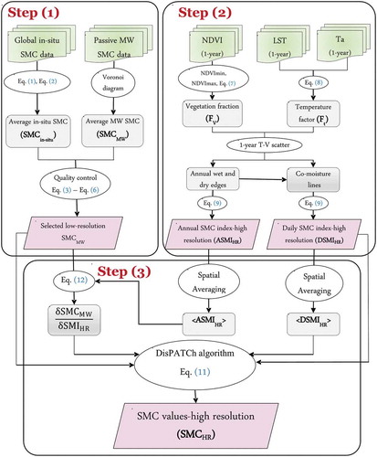
According to Figure 3, the proposed method can be categorized in the following steps:

1. Selecting an appropriate MW soil moisture product: Using the global in situ SMC networks, this step evaluates and compares the different passive MW soil moisture products in light of quality, correlation coefficient, and possible errors leading to identify the most accurate one.

2. Calculating the high-resolution SMC indices: In this step, the novel annual and daily SMC indices are introduced and calculated by the wet edge, dry edge, and co-moisture lines attained from the 1-year T-V scatter plot introduced in Mohseni and Mokhtarzade (2020).

3. Providing absolute SMC values: Coarse-scale MW soil moisture products are integrated by high-resolution SMC indices into a downscaling algorithm to provide absolute SMC values at intermediate spatial resolution. In so doing, DisPATCh is applied as the downscaling algorithm with a novelty to identify the relationship between high-resolution indices and coarse-scale microwave SMC images.

Step 1: selecting the appropriate satellite-based passive microwave SMC products

The main achievement of the proposed method is to attain the absolute SMC values at high spatial resolution using SMC indices extracted from the T-V scatter plot and passive MW soil moisture (SM_MW) measurements. It is obvious that the accuracy of coarse-scale SM_MW products directly governs the accuracy of resultant high-resolution SMC values (Djamai et al. 2016). Therefore, it is very important to select and apply an SM_MW that accurately measures the soil moisture. So far, a vast number of studies have been carried out to evaluate and compare various passive microwave SMC products (Al-yaari et al. 2014, Chan et al., 2016; Chen et al. 2018, Grant et al., 2016; Jackson et al. 2014, Cui et al., 2017; Cui et al. 2018, Ma et al., 2019, Yee et al., 2017; Kim et al. 2018). Almost all of these papers acknowledged that among the SM_MW retrieved from various available passive MW sensors, the products of AMSR2, SMOS, and SMAP had the best accuracy for monitoring SMC at the various study areas (Jackson et al. 2014; Zhang, Kim, and Sharma 2019; El Hajj et al. 2018). Accordingly, in this study, appropriate SM_MW is selected among from the SMC products of AMSR2, SMOS, and SMAP satellites, which are found as the most accurate ones. In so doing, their products are compared with ground-based measurements on a global scale and at a relatively long time interval.

Similar to the other assessments of remote sensing data, mismatching the spatial scale of point-based in situ measurements with satellite-based observations, which is approximately 25–50 km for MW products, is a major concern (Merlin et al. 2012; Kerr et al. 2016a). To address this issue, the stationary in situ measurements must be upscaled to obtain an accurate estimate of the in situ soil moisture within the microwave coarse-scale grid.

In this study, we applied a combined upscaling technique, in which the inverse-distance-weighted average of the in situ measurements is calculated for the mean center of the validation site. The main purpose of this method is to apply the maximum number of stations with the highest spatial distribution on a validation site. In this technique, the weighted average of those stations located in a microwave grid size is calculated at the geographic center of the validation site (Eq. (1)(1) $SM{C}_{insitu}=\frac{\sum _{i=1}^n{P}_i\times S{M}_i}{\sum _{i=1}^n{P}_i}$(1) ).

(1) $SM{C}_{insitu}=\frac{\sum _{i=1}^n{P}_i\times S{M}_i}{\sum _{i=1}^n{P}_i}$(1)

where n is the number of those stations that are located in a spatial extent of the microwave grid size (36 km for SMAP, 25 km for SMOS, and 0.25º for ASMR2 validation). The SM_i and P_i values are respectively the point measurement of ith station and its weight, which is calculated by Eq. (2)(2) $p_i=\frac{1}{\sqrt{{(x_i-x_o)}^2+{(y_i-y_o)}^2}}$(2) .

(2) $p_i=\frac{1}{\sqrt{{(x_i-x_o)}^2+{(y_i-y_o)}^2}}$(2)

With (x_i,y_i) and (x_o,y_o) being the geographical location of the corresponding station and the geographic center of the in situ sites, respectively. For a visual explanation, Figure 4 shows all stations of the Kenaston network and those stations located in an EASE-Grid 2.0 grid size (36 km). Given Figure 2, Kenaston network, also called the Brightwater Creek (Tetlock et al. 2019), is one of the study sites that is applied to evaluate the SMC values derived from passive MW remote sensing satellites (site ID 28 in Figure 2). For Kenaston agricultural network, which is located on the Canadian prairies in central Saskatchewan, the ground measurements of soil moisture are available for 45 fields at a depth of 0–5 cm. The stations within the network were set at two spatial scales (Kolassa et al. 2018). The mean center of this network is shown with a green point in Figure 4. According to Figure 4, from all 45 sites of Kenaston, 39 stations shown with red points are located in an EASE-Grid 2.0 grid size (filled blue rectangle in Figure 4). The weighted average of the in situ measurements is calculated based on the distance between the center of the network and the corresponding stations.

Figure 4. The Kenaston field campaign. Those stations distributed in an area equal to the standard MW product grid size (filled blue rectangle) are selected for the validation process. Lines show the SMAP global grid area

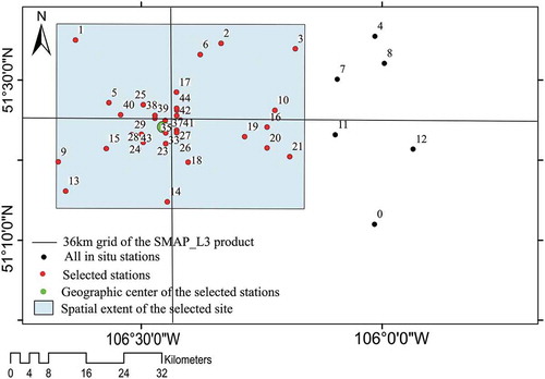
In the case of SM_MW, in which the distribution of the data (e.g. the center of MW grid) is uniform, the Voronoi diagram algorithm is applied to calculate the weighted average (Colliander et al. 2017). In this algorithm, the weight of each pixel directly depends on the range of the spatial extent of the site that it covers. More information on the Voronoi diagram method is available in Secord (2002). It must be mentioned that even though SMAP, SMOS, and AMSR2 missions have some systematic differences in adopted radiometer instruments (band, polarization, resolution, radiometric uncertainty), orbit parameters (orbit altitude, inclination, local time of ascending node), and the strategies of observation recording; however, all of them are the gridded datasets that are disseminated on some global map projection. Therefore, in this step, which is a re-gridding process of the MW products, it is not necessary to consider the systematic differences between those products.

The accuracy in SM_MW products is validated by several statistical indicators, such as correlation coefficient (R), mean difference (bias), root mean square difference (RMSE), and unbiased RMSE (ubRMSE) (Eqs. (3)–6)) in a quality control procedure (Al-yaari et al. 2014; Zhang, Kim, and Sharma 2019).

(3) $R=\frac{\sum _{i=1}^n(SM{C}_{insitu,i}-\overline{SM{C}_{insitu}})(S{M}_{MW,i}-\overline{S{M}_{MW}})}{\sqrt{\sum _{i=1}^n{(SM{C}_{insitu,i}-\overline{SM{C}_{insitu}})}^2}\sum _{i=1}^n{((S{M}_{MW,i}-\overline{S{M}_{MW}}))}^2}$(3)

(4) $Bias=\frac{1}{n}\sum _{i=1}^n(S{M}_{MW}-SM{C}_{insitu})$(4)

(5) $RMSE=\sqrt{\frac{1}{n}\sum _{i=1}^n{(S{M}_{MW}-SM{C}_{insitu})}^2}$(5)

(6) $ubRMSE=\sqrt{RMS{D}^2-Bia{s}^2}$(6)

where n is the number of days in which their remote sensing observations are used in the validation process. Concerning these indicators and statistical analyses related to them, the most accurate SMC product is identified as the output of the step 1 and is applied in the next steps of the proposed method. Figure 3 emphasizes the general procedure for identifying the most accurate SM_MW as step 1. Note that, in order to achieve an accurate assessment, in situ SMC measurements recorded at 6:00 a.m. (SMAP descending and SMOS ascending overpass time) and at 1:30 a.m. (AMSR2 ascending overpass time) are applied to validate SMAP, SMOS, and AMSR2 soil moisture products, respectively.

Step 2: obtaining SMC indices from long-term T-V scatter plot

The T-V scatter plot method is used to obtain a high-resolution SMC index. The main concept of the T-V scatter plot method is that the scatter plot of surface temperature factor against vegetation fraction cover has a construction similar to a triangle or a trapezoid with two edges: the dry edge represents zero SMC and minimum evapotranspiration and the wet edge indicates maximum evapotranspiration and adequate SMC (Carlson, Gillies, and Perry 1994; Patel, Mukund, and Parida 2019). According to this theory, the SMC of each point is directly related to the distance from that point to the dry and wet edges (Carlson, Gillies, and Schmugge 1995). Generally, the T-V scatter plot method includes two main processes, determining the wet and dry edges and estimating the SMC index based on the interpolation between the dry and wet edges (Zhang and Zhou 2016). Therefore, the reliability of every SMC index extracted from T-V scatter plot is mainly governed by the accuracy of the wet and dry edges definitions (Mohseni and Mokhtarzade 2020). As such, in those conditions that the wet and dry edges are not well extractable, the T-V method is inoperative.

Starting from Carlson (2007) and related researches (Minacapilli et al. 2016; Liu and Yue 2018; Zhu, Jia, and Lv 2017a), in our study we applied a long-term T-V scatter plot suggested by Mohseni and Mokhtarzade (2020). A long-term T-V scatter plot is created using the EOs over a longer period of time instead of a single day. The main theoretical premise behind the long-term T-V scatter plot method is the existence of pixels with comprehensive humidity conditions that decrease the requirement for the axillary in situ data to extract accurate wet and dry edges. In light of that the temperature and vegetation data of 1-year provide almost all comprehensive information about the occurrence of humidity and the vegetation conditions (e.g. dry soil, saturated soil, healthy vegetation and stressed vegetation), Mohseni and Mokhtarzade (2020) argued that 1-year interval is the optimum period, leading to well-defined annual wet and dry edges.

In line with previous 1-year T-V scatter plot, the normalized NDVI calculated by the minimum (NDVI_min) and maximum (NDVI_max) NDVI over the 1-year interval is considered as the vegetation factor (Fv), and hence the horizontal axis (Eq. (7)(7) $Fv=\frac{NDVI-NDV{I}_{min}}{NDV{I}_{max}-NDV{I}_{min}}$(7) ).

(7) $Fv=\frac{NDVI-NDV{I}_{min}}{NDV{I}_{max}-NDV{I}_{min}}$(7)

On the other hand, based on the (Mohseni and Mokhtarzade 2020) resultants, which find the daytime surface–air temperature gradient as the best temperature factor for monitoring soil moisture condition, temperature factor (Ft) and the vertical axis are derived as Eq. (8)(8) $Ft=LS{T}_{daytime}-Ta{\hspace{0.17em}}_{daytime}$(8) .

(8) $Ft=LS{T}_{daytime}-Ta{\hspace{0.17em}}_{daytime}$(8)

With LST being the satellite-derived daytime land surface temperature and, also, Ta being the ground-based measurements of air temperature at satellite overpass time. As mentioned before, to minimize the LST data gaps due to cloud cover, we applied both LST products of MODIS/Terra (10:30 a.m. local time) and MODIS/Aqua (1:30 p.m. local time). It means that in those days when MODIS/Terra data have more than 20% cloud cover, MODIS/Aqua data were downloaded and applied. Depending on the MODIS LST products, Ta at 10:30 a.m. or 1:30 p.m. is used to calculate Ft. After a sensitivity analysis, we realized that although the use of two different times for Ft calculation creates some uncertainties in SMC measurements, these uncertainties are less than the relative error of SM_MW, (0.04 m³/m³) and therefore are negligible.

In order to retrieve the SMC index from 1-year T-V scatter plot, the well-known linear relationship between vegetation factor, temperature factor, and SMC, which is established by Sandholt, Rasmussen, and Andersen (2002), is applied. The conceptual theory of this relationship has been widely applied to introduce different SMC indices (Petropoulos, Ireland, and Barrett 2015). According to this theory, the locus of points within the same soil moisture or vegetation water content is a unique line between the dry and the wet edge so that the SMC of the corresponding line depends on the distance to those edges (Moran et al. 1994; Yang et al. 2015; Sadeghi et al. 2017) . Given that, for each point in the T-V scatter plot, the high-resolution SMC index (SMI_HR) is calculated using Eq. (9)(9) $SM{I}_{HR}=\frac{F{t}_i-F{t}_{min}}{F{t}_{max}-F{t}_{min}}=\frac{F{t}_i-(a_{wet}\times F{v}_i+b_{wet})}{(a_{dry}\times F{v}_i+b_{dry})-(a_{wet}\times F{v}_i+b_{wet})}$(9) .

(9) $SM{I}_{HR}=\frac{F{t}_i-F{t}_{min}}{F{t}_{max}-F{t}_{min}}=\frac{F{t}_i-(a_{wet}\times F{v}_i+b_{wet})}{(a_{dry}\times F{v}_i+b_{dry})-(a_{wet}\times F{v}_i+b_{wet})}$(9)

where Ft_i and Fv_i are the temperature and vegetation factors for the ith pixel, respectively. Note that since both Fv and Ft are derived from 1 km MODIS products, Eq. (9)(9) $SM{I}_{HR}=\frac{F{t}_i-F{t}_{min}}{F{t}_{max}-F{t}_{min}}=\frac{F{t}_i-(a_{wet}\times F{v}_i+b_{wet})}{(a_{dry}\times F{v}_i+b_{dry})-(a_{wet}\times F{v}_i+b_{wet})}$(9) calculates the SMI_HR values at the spatial resolution of 1 km. a_dry and b_dry are the parameters of the dry edge. a_wet and b_wet, on the other hand, represent the parameters of the wet edge. Depending on to the wet and dry edges applied to calculate SMC indices, two different types of SMI_HR are introduced and extracted from the proposed 1-year T-V scatter plot: annual SMC index (ASMI_HR) and daily SMC index (DSMI_HR).

ASMI_HR, showing the SMC rate of one point relative to the conditions over the entire year interval, is calculated using the edges of a 1-year T-V scatter plot referred to as the “annual wet edge” and “annual dry edge.” The annual dry and wet edges are extracted from the 1-year scatter plot following the approach presented in (Merlin et al. 2012) and applied in (Mohseni and Mokhtarzade 2020). According to (Merlin et al. 2012), the line that passes through (1, Ft_v,min), and at the same time, is placed under all other points with Fv< 0.5, is considered as the annual wet edge. Ft_v,min represents the vegetation temperature at minimum water stress and is equal to the minimum Ft over the time period in which the T-V scatter plot is produced. Also, annual dry edge is considered as the line that passes through (1, Ft_v,max) so that all pixels with Fv < 0.5 are located below it. Ft_v,max, which refers to the temperature factor of a vegetated pixel with the highest water stress, is calculated by Eq. (10)(10) $F{t}_{v,max}=max(\frac{Ft-max(Ft)\times (1-Fv)}{Fv})$(10) .

(10) $F{t}_{v,max}=max(\frac{Ft-max(Ft)\times (1-Fv)}{Fv})$(10)

For a visual explanation, Figure 5 shows the parameters Ft_v,max, Ft_v,min, the annual wet edge, and the annual dry edge of a hypothetical 1-year scatter plot.

Figure 5. A typical 1-year T-V scatter plot with its annual wet and dry edges and some imaginary co-moisture lines between them. A hypothetical 1-day scatter plot and the daily wet and dry edges are also shown in this figure

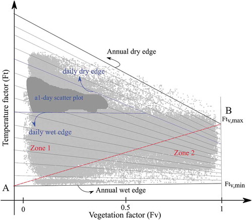
DSMI_HR, on the other hand, describes the humidity condition of a specific point in one particular day relative to the other points of the corresponding date. DSMI_HR is calculated using the unique wet and dry edges of the 1-day scatter plot. In so doing, the daily wet edge is considered as a horizontal line that passes through the minimum value of the surface–air temperature gradient of the T-V scatter plot of the corresponding day.

To achieve the daily dry edge, a concept, referred to as the “co-moisture line,” is employed. Co-moisture lines are the locus of points with an equal SMC index that is located between the annual wet and dry edges. Figure 5 shows some hypothetical co-moisture lines, each of which has a unique SMC index value in range 0 and 1. For a specific day, the dry edge is selected among from all co-moisture lines in such a way that all points with Fv < 0.5 belonging to the corresponding day are located below it. For more clarification, Figure 5 also shows a simulated 1-day T-V scatter plot and the selected co-moisture line as the dry edge.

It must be kept in mind that the DSMI_HR values are not related and comparable with ASMI_HR until it converts the absolute SMC values using the Disaggregation based on Physical and Theoretical scale Change (DisPATCh) algorithm. The underlying concept is that ASMI_HR is calculated using the annual wet and dry edges of a 1-year T-V scatter plot, in which the pixels related to dry and wet conditions happen at the top and bottom of the trapezoidal chart, respectively. However, DSMI_HR emphasizing the humidity condition of a specific point in one particular day relative to the other points extends in range 0 and 1, even when there is no saturated and dry condition within a coarse-scale MW grid. As a result, one can conclude that although ASMI_HR describes the SMC rate of one point relative to the conditions over the entire year interval, DSMI_HR shows only the numbers between zero and one, which only makes sense along with the soil moisture values obtained by MW coarse-scale grid. The general procedure for determining annual and daily SMC indices is given in Figure 3 (step 2).

Step 3: providing absolute SMC values

As the last step of our proposed method, the DSMI_HR index is converted to the absolute SMC value. To this end, we applied DisPATCh, proposed by Merlin et al. (2008, 2010, 2012). More specifically, DisPATCh is employed as a downscaling algorithm to disaggregate the coarse-scale passive SMC products to the high-resolution SMC maps using optical/thermal-derived soil moisture index given a first-order Taylor series approximation around the coarser-scale MW pixel (Eq. (11(11) $\mathrm{S}\mathrm{M}{\mathrm{C}}_{\mathrm{H}\mathrm{R}}=S{M}_{MW}+\frac{\mathrm{\partial }S{M}_{MW}}{\mathrm{\partial }SM{I}_{HR}}\times (DSM{I}_{HR}-⟨DSM{I}_{HR}⟩)$(11) )) (Malbéteau et al. 2016; Neuhauser et al. 2019).

(11) $\mathrm{S}\mathrm{M}{\mathrm{C}}_{\mathrm{H}\mathrm{R}}=S{M}_{MW}+\frac{\mathrm{\partial }S{M}_{MW}}{\mathrm{\partial }SM{I}_{HR}}\times (DSM{I}_{HR}-⟨DSM{I}_{HR}⟩)$(11)

where SM_MW is the low-resolution soil moisture value of those products that are selected in step 1, DSMI_HRis daily soil moisture index extracted from 1-year T-V scatter plot at spatial resolution of MODIS products, <DSMI_HR> is the average of high-resolution soil moisture index within a coarse-scale microwave pixel, and ∂SM_MW/∂SMI_HR is the partial derivative of SM_MW relative to SMI_HR. More briefly, the ∂SM_MW/∂SMI_HR is a linking term between the SMC index and low-resolution soil moisture values. There is a considerable amount of literature on multiple linear and nonlinear regressions to estimate the ∂SM_MW/∂SMI_HR values. Since the underlying assumption in using the co-moisture lines to calculate the SMC indices is the existence of a linear relationship between the T-V indices and the SMC values, in this paper, the corresponding term is computed via a novel method using the linear regression between annual soil moisture indices extracted from 1-year interval T-V scatter plot and soil moisture measurements of microwave satellite over a 1-year period (Eq. (12)(12) $\frac{\mathrm{\partial }S{M}_{MW}}{\mathrm{\partial }SM{I}_{HR}}=\frac{1}{N}\times \sum _{i=1}^N(\frac{S{M}_{MW,i}}{<ASM{I}_{HR,i}>})$(12) ).

(12) $\frac{\mathrm{\partial }S{M}_{MW}}{\mathrm{\partial }SM{I}_{HR}}=\frac{1}{N}\times \sum _{i=1}^N(\frac{S{M}_{MW,i}}{<ASM{I}_{HR,i}>})$(12)

In Eq. (12(12) $\frac{\mathrm{\partial }S{M}_{MW}}{\mathrm{\partial }SM{I}_{HR}}=\frac{1}{N}\times \sum _{i=1}^N(\frac{S{M}_{MW,i}}{<ASM{I}_{HR,i}>})$(12) ), N represents the total number of days during the year that was used to solve the ∂SM_MW/∂SMI_HR. Note that for each coarse-scale SMAP pixel, the ∂SM_MW/∂SMI_HR value is unique and is calculated separately from other pixels. Figure 3 (step 3) summarizes the general procedure for determining the high-resolution SMC maps using SMC indices derived from the proposed 1-year T-V scatter plot and low-resolution MW soil moisture products. It must be mentioned that since the products of MODIS Aqua, MODIS Terra, and MW SMC measurements, each of which has different overpass time (see Section 2.3), are applied to estimate high-resolution soil moisture data, in situ soil moisture obtained at 10 a.m., which is almost the middle of the data acquisition times, is used to evaluate the resultants of the proposed method.

Results and discussion

Step 1: global-scale evaluation of SMOS, AMSR2, and SMAP SMC products

Among all the sites presented in Figure 2, those that meet all of the validation site requirements argued by Jackson et al. (2010) were selected (see Section ‎2.2) and applied to estimate the total accuracy of SM_MW. Table 1 lists all the detailed information of those selected sites. The column “Site No” in Table 1 presents the number by which each site is displayed in Figure 2.

Table 1. SM_MW validation sites with the number by which they are shown in Figure 2

Site no.	Site name	Country	Location of center		Climate regime	N1^1	N2^2	Period	Reference
			Latitude (N)	Longitude (E)
1	OZNET	Australia	−34.858	146.145	Semi-arid temperate	38	25	5/4/2015- 12/31/2018	(Smith et al. 2012)
			−35.338	147.515
6	CTP_SMTMN	China	31.733	91.783	Cold and humid	57	23	5/4/2015- 9/19/2016	(Yang et al. 2013)
16	HOBE	Denmark	55.969	9.097	Temperate-maritime	32	32	5/4/2015- 12/31/2018	(Bircher et al. 2012)
22	REMEDHUS	Spain	41.316	−5.372	Temperate	24	19	5/4/2015- 12/31/2018	(Sánchez-ruiz et al. 2014)
26	SMAPVEX16-MB	Canada	42.452	−93.342	Arid	50	50	5/28/2016- 8/16/2016	(Hornbuckle et al. 2017)
27	RISMA	Canada	49.608	−97.945	Temperate	23	9	5/4/2015- 2/9/2017	(Bhuiyan et al. 2018)
28	Kenaston	Canada	51.427	−106.411	Cold	45	39	5/4/2015- 9/30/2017	(Rowlandson et al. 2015)
34	Walnut Gulch	USA	31.721	−110.031	Arid	21	19	5/4/2015- 12/31/2017	(Jackson et al. 2010)
^1Total number of SMC estimation stations in each site.
^2Number of stations employed in the validation process.

In Table 1, N₁ refers to the total number of stations in each site. Moreover, N₂ presents the number of stations of each sites that are located within a SMAP cell (approximately 36 km). Those stations that are located at a spatial extent of radiometer footprint size are employed in the validation process. To this end, the geometric center of each site was defined in ArcGIS and then used as the center of a square with a side length of microwave grid size. All of the stations, which are located in the corresponding square, were employed to calculate the average in situ SMC for the validation process (the column “N₂” in Table 1). As can be seen, there are at least nine stations in each validation site leading to 70% confidence for 0.03 m³/m³ soil moisture uncertainty with 0.07 m³/m³ variability (Colliander et al. 2017). Notably, according to the column “Period” in Table 1, almost all of those selected sites are planned and constructed to measure SMC at a long time series. These features, along with variations in the climate classification of study sites (see column “climate regime” in Table 1), allow for a comprehensive and dependable assessment of the SM_MW at a wide range of soil moisture, vegetation density, land surface temperature, and climate conditions (Zhang, Kim, and Sharma 2019).

Figure 6 presents the results of the spatial correlation analyses performed between the SM_MW products and the corresponding soil moisture measurements, separately for eight validation sites, each of which is shown in an individual chart. It should be noted that the results of Figure 6 were obtained using data from those days in which both in situ measurements and satellite images were available. On the other hand, According to Djamai et al. (2016), all SM_MW data with the Data Quality index (DQX) values above a threshold of 0.06 m³/m³ or a DQX of −999 were discarded to increase the accuracy of assessments. The bold lines on the cloud points are the linear regression lines and the gray lines are the lines of y = x with the slope of one.

Figure 6. Scatter plots of daily soil moisture estimates from field stations versus AMSR2, SMOS, and SMAP soil moisture products at eight validation sites

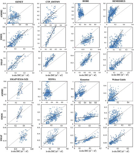
Regarding these linear regression lines and distribution of the cloud points, AMSR2 has relatively poorer performance than other sensors in SMC estimation. In some sites, like HOBE and RISMA, there even a negative or zero correlation between AMSR2 soil moisture measurements and in situ SMC. However, in SMAPVEX16-MB, all three sensors have the same performance. To more clarify the performance of various SM_MW, Table 2 details the resultant statistical scores, such as R, RMSE, bias, and unbiased RMSE, with the best values shown in bold.

Table 2. Summarized resultant statistical indicators for the AMSR2, SMOS, and SMAP products

Statistical metrics of different satellite		OZNET	CTP_SMTMN	HOBE	REMEDHUS	SMAPVEX16-MB	RISMA	Kenaston	Walnut Gulch	Average
R	AMSR2	0.24	0.53	−0.3	0.63	0.55	0.03	0.45	0.46	0.32
	SMOS	0.81	0.83	0.53	0.72	0.30	0.55	0.24	0.53	0.56
	SMAP	0.84	0.93	0.73	0.81	0.64	0.53	0.55	0.78	0.73
RMSE (m^3/m^3)	AMSR2	0.16	0.11	0.28	0.12	0.12	0.26	0.25	0.08	0.17
	SMOS	0.07	0.14	0.07	0.06	0.19	0.09	0.12	0.05	0.10
	SMAP	0.07	0.12	0.08	0.04	0.09	0.09	0.05	0.03	0.07
Bias (m^3/m^3)	AMSR2	0.04	−0.02	0.20	0.12	0.03	0.18	0.20	0.01	0.10
	SMOS	0	0.13	−0.05	−0.03	−0.05	−0.04	−0.01	0.01	−0.01
	SMAP	0.02	0.08	0.05	0	0.01	0.02	−0.03	0.02	0.02
ubRMSE (m^3/m^3)	AMSR2	0.16	0.11	0.18	0.09	0.11	0.18	0.14	0.08	0.13
	SMOS	0.07	0.05	0.05	0.05	0.18	0.08	0.12	0.05	0.08
	SMAP	0.06	0.08	0.06	0.04	0.09	0.09	0.05	0.02	0.06

According to Table 2, some clear-up conclusions can be drawn and summarized as follows: as it was explained through Figure 6, regarding the correlation coefficients (R), there is the lowest agreement of the AMSR2 soil moisture products and the in situ data in all validation sites. The correlation coefficient between in situ and AMSR2 measurements has even a negative value in HOBE station. In this regard, SMAP products outperform the other products in nearly all sites, except RISMA, where SMOS has better performance. Given the better performances of L-band – at which the SMOS and SMAP are operated – than other passive microwave bands in retrieving SMC, these results are not surprising (Kerr et al. 2010; Kumar et al. 2018). In addition, Figure 6 yields to the improvement of these claims, where there is a much closer agreement of the SMAP soil moisture products and the in situ data.

Regarding the RMSE, SMAP products show better results in the four sites of eight validation sites, including REMEDHUS, SMAPVEX16, Kenaston, and Walnut Gulch. note that in these mentioned sites, there are small quantitative differences between SMAP and SMOS resultants, which is in line with Entekhabi et al. (2014)‘s argument. Moreover, SMAP and SMOS have same RMSE in OZNET and RISMA.

One interesting subject fundable from Table 2 is that not only do none of the MW missions meet the mentioned nominal error (RMSE better than 0.04 m³/m³), but they also have different performances in various validation sites. This issue is maybe because of the various static and dynamic conditions, such as vegetation cover, soil temperature, and climate condition (Zhang, Kim, and Sharma 2019; Petropoulos, Ireland, and Barrett 2015). However, slightly poor results are found from the AMSR2 in all validation sites, except CTP_SMTMN. Bias values gathered in Table 2 are strong evidence of this issue. According to Table 2, for five validation sites, the |bias| values of AMSR2 are equal to and larger than the nominal error of microwave soil moisture measurement.

ubRMSE, on the other hand, is a bias-corrected RMSE of SM_MW. Using RMSE and bias, the ubRMSE, which is the standard deviation of the differences between the SM_MW and ground-based measurements, was calculated (Eq. (6)(6) $ubRMSE=\sqrt{RMS{D}^2-Bia{s}^2}$(6) ). Similar to the statistical analyses related to RMSE, lower values of this indicator imply more reliable and accurate measurements (Kerr et al. 2016a). According to Table 2, in almost all sites, the SMAP and SMOS have the lowest ubRMSE and AMSR2 has the highest ubRMSE. Regarding all mentioned statistical indicators and according to the results of Table 2, it can be concluded that AMSR2 cannot be a proper candidate for microwave SMC products.

Even though there is almost similar performance between SMAP and SMOS resultants, however, the question under discussion is that which one of them is more accurate? To answer this question, Figure 7 summarizes all mentioned conclusions drawn from Table 2 and Figure 6 as the percentage of statistical indicators where a given microwave SMC product outperforms another one.

Figure 7. Percentage of cases where SMAP or SMOS products rank best

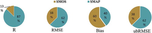
Figure 7 argues the superiority of the SMAP products, which performs better than SMOS products in terms of the correlation coefficient, RMSE, and ubRMSE by more than 62% m³/m³ on average. As stated by Abbaszadeh, Moradkhani, and Zhan (2019), this is likely because the SMOS observations are more sensitive to RFI distortion than SMAP products, especially over densely vegetated areas. According to the SMAP advantages mentioned above, in the remaining analysis of this paper, SMAP was applied as the SM_MW for calculating the high-resolution SMC map.

Step 2: retrieving annual and daily SMC indices from 1-year T-V scatter plot

Annual T-V scatter plots and the corresponding annual wet and dry edge are presented in Figure 8 (a). This scatter plot is made up of 81 non-cloudy images of the year 2016 for the SMAPVEX16-MB network. The spatial extent of the MODIS images, over which the T-V scatter plot is formed, corresponds to the one SMAP product grid size (36 km).

Figure 8. (a) A 1-year scatter plot for the SMAPVEX16 site formed by 81 remote sensing images of the year 2016. (b–f) T-V scatter plot for some days of the year 2016 for the corresponding network. The dotted and solid lines represent annual and daily edges, respectively

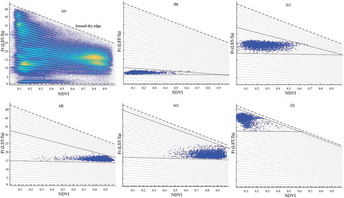
Figure 8 also shows the daily T-V scatter plots of some several days in 2016, their horizontal wet edges, and even their dry edges, which were selected from co-moisture lines in such a way that explained in Section 3.2. Table 3 details the air temperature, vegetation, and soil moisture conditions of the corresponding days.

Table 3. An inspection of ground-based soil moisture, air temperature, and satellite-based vegetation conditions of 5 days that their daily scatter plots are presented in Figure 8

	Date	NDVI			Volumetric SMC (m^3/m^3)			Ta10:30am (°C)
		Min	Max	Mean	Min	Max	Mean
(b)	15 November 2016	0	0.68	0.20	0.14	0.47	0.28	7.51
(c)	30 April 2016	0	0.72	0.32	0.08	0.24	0.16	0.31
(d)	22 July 2016	0.17	0.98	0.81	0.18	0.43	0.31	16.94
(e)	4 August 2016	0.40	1	0.77	0.11	0.34	0.28	15.88
(f)	5 January 2016	0	0.77	0.12	0.03	0.22	0.13	0.69

As mentioned in the Introduction, one of the limitations of the traditional T-V scatter plot is the low accuracy of determining the wet and dry edges of the scatter plot in cases that these edges are not formed appropriately due to the lack of comprehensive vegetation and temperature. In these situations, the accuracy of the T-V scatter plot method is not reliable. In line with Figure 8 along with NDVI and SMC information given in Table 3, this issue is immediately apparent. As can be seen, none of the isolated 1-day scatter plot has the comprehensive humidity and vegetation conditions to define the correct trapezoidal shape and consequently accurate dry and wet edges. In these conditions, determining the right theoretical dry edge requires some additional environmental parameters.

This limitation is addressed by use of a 1-year scatter plot in which a well-known trapezoidal shape and its edges are correctly formed thanks to the more humidity and vegetation situation occurring in the 1-year interval. This result provides strong evidence that the long-term T-V scatter plot is more suitable than the traditional 1-day scatter plot for estimating and extracting various kinds of SMC indices introduced before. This point corroborates previous results (Mohseni and Mokhtarzade 2020).

According to Table 3 and Figure 8, the pixels related to the drier days (e.g. 5 January) happen at the upper part of the annual scatter plot and lead to form an accurate annual dry edge. The pixels belong to the wet dates (e.g. 15 November), contrariwise, happen at the lower parts of the 1-year scatter plot and create the annual wet edge. As a result, we claim that ASMI_HR, which is calculated using annual wet and dry edges, is directly related to the wetness condition of the soil over 1-year interval. As some arguments of this claim, Figure 9 and Figure 10 are presented.

Figure 9. ASMI_HR maps of (a): 1 May 2016, (b) 10 September 2016, (c) 15 October 2016, and (d) 18 July 2016. The corresponding maps are retrieved through the 1-year scatter plot and calculated by the annual wet and dry edge

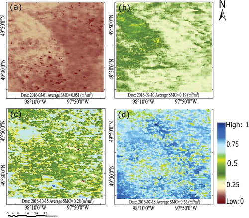
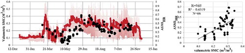
Figure 10. Time-series comparison between ASMI_HR index derived from the 1-year scatter plot and in situ SMC measurements. In situ measurements and estimated ASMI_HR are shown with red continues line and black circles, respectively. The average SMC values are derived from the SMC of the nine in situ stations for each day, also, the average values of the calculated index, computed over nine image pixels containing the corresponding stations

Figure 9 shows the ASMI_HR maps of 4 days and their corresponding average in situ SMC measurements at the SMAPVEX16 site during 2016. The ASMI_HR maps of Figure 9 provide convincing evidence that the annual SMC indices of various days are the proxies of the humidity of those days relative to the rest of the year and, therefore, temporarily comparable. Given Figure 9, the ASMI_HR map of 1 May, which is the driest day among all of the mentioned ones (average SMC equal to 0.05), has the lowest ASMI_HR values. Soil moisture index values gradually increase in the next three maps until the ASMI_HR values of 18 July, as the wettest day, exhibit the highest values. Therefore, the annual SMC indices of all 4 days are temporarily comparable. This issue is against previous SMC indices extracted from the 1-day scatter plot. In traditional 1-day T-V scatter plot method, the SMC indices of each day take all the values in the range between zero and one, regardless of the humidity of that day relative to the rest of the year. On the other hand, various T-V scatter plots were used to calculate the SMC indices of various days. It means that each day has its own T-V scatter plot and wet and dry edges. These issues make it impossible to compare between the maps of different days.

More broadly, the time series of the average in situ SMC data estimated by RISMA stations, together with the average ASMI_HR indices extracted from the 1-year scatter plot, is shown in Figure 10.

Figure 10 shows an excellent consistency between relative soil wetness conditions over a year and the ASMI_HR maps calculated by the annual wet and annual dry edge. Along a similar line, we can argue that there is also a precise relationship between this index and the amount of soil moisture retrieved from passive microwave satellites.

However, as can be seen from the right vertical axes of Figure 10, the indices extracted from the long-term T-V scatter plot are still some dimensionless proxy of the SMC in range of 0–1 and are not the absolute SMC values. As mentioned in the introduction section, this is the third limitation of the T-V scatter plot that tried to be addressed in this study. In the next step of the proposed method, these indices will be converted to the absolute SMC values using coarse-scale SM_MW.

In the case of DSMI_HR, the daily dry and wet edge were used to calculate the SMC index (see Figure 8). By considering daily wet and dry edges in calculating SMC indices, DSMI_HR values extend in the range 0 and 1, even when there is no saturated and dry condition within a coarse-scale MW grid.

This is against the annual SMC indices, which may take a number in the range between less than 0–1 (e.g. 0.1 and 0.3) based on its distance to the annual edges (see Figure 9). It can be concluded that DSMI_HR is not comparable with ASMI_HR, also in situ SMC values. Therefore, this index will be investigated in the following section, after converting it to the absolute SMC values.

Step 3: providing absolute SMC values

Results of the parameter ∂SM_MW/∂SMI_HR

As described in Section 3.3, DisPATCh was applied to convert the high-resolution SMC indices into the absolute SMC values. In so doing, firstly, the relationship between soil moisture values of the coarse-scale SMAP pixels and the average of the high-resolution SMC indices within them – as the parameter ∂SM_MW/∂SMI_HR – must be defined. As mentioned earlier, current research innovatively applies the linear relationship between average ASMI_HR indices and SMAP observations to calculate ∂SM_MW/∂SMI_HR (Eq. (12)(12) $\frac{\mathrm{\partial }S{M}_{MW}}{\mathrm{\partial }SM{I}_{HR}}=\frac{1}{N}\times \sum _{i=1}^N(\frac{S{M}_{MW,i}}{<ASM{I}_{HR,i}>})$(12) ).

Figure 11 gives the results of the linear correlation analysis between soil moisture estimates of four coarse-scale SMAP pixels covering the study area and the average of ASMI_HR indices within them. Since the parameter ∂SM_MW/∂SMI_HR is unique for each SMAP pixel (Merlin et al. 2012), the points related to four SMAP pixels are shown by different colors in Figure 11.

Figure 11. 36 km SMC values retrieved by SMAP mission versus the average of (a) LST, (b) Ft (LSTdaytime – Ta (10:30 a.m.)), (c) Fv (normalized NDVI), and (d) annual SMC index extracted from 1-year T-V scatter plot. Four lines in each diagram are the linear regression lines belonging to the four SMAP pixels

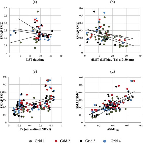
Table 4 expands on the correlation analysis between SMAP soil moisture measurements and the average of LST, Ft, and Fv estimations, separately for four SMAP grids.

Table 4. The results of the correlation analysis between the soil moisture retrieval of four pixels of SMAP products and Fv, Ft, LST and ASMI_HR over the study area

	LST (10:30)	Ft	Fv	ASMIHR	Line
Grid 1	0	0.24	0.52	0.73	Y = 0.532 × X + 0.0015
Grid 2	0.28	0.22	0.53	0.72	Y = 0.3968 × X + 0.0795
Grid 3	0.31	0.42	0.49	0.70	Y = 0.48 × X + 0.075
Grid 4	0.11	0.60	0.49	0.64	Y = 0.42 × X + 0.071
Average	0.15	0.37	0.51	0.70

The linear regression equations for the best-fitted straight lines between ASMI_HR and SMAP are listed in the last column of Table 4. X and Y represent the ASMI_HR index and SMAP soil moisture observation, respectively. The slopes of these lines were considered as the parameter ∂SM_MW/∂SMI_HR of each SMAP pixels and are used in Eq. (11)(11) $\mathrm{S}\mathrm{M}{\mathrm{C}}_{\mathrm{H}\mathrm{R}}=S{M}_{MW}+\frac{\mathrm{\partial }S{M}_{MW}}{\mathrm{\partial }SM{I}_{HR}}\times (DSM{I}_{HR}-⟨DSM{I}_{HR}⟩)$(11) to calculate high-resolution SMC values. The obvious conclusion that can be drawn from Table 4 and Figure 11 is the superiority of the proposed temperature factor (LST-Ta), which performs better than LST in terms of the correlation coefficient by more than 0.22 on average. As a result, one can argue that compared to the LST, the surface–air temperature gradient is more appropriate to apply in the T-V scatter plot method and to estimate the SMC index. This point corroborates previous results (Rahimzadeh-bajgiran, Omasa, and Shimizu 2012; Rahimzadeh-bajgiran et al. 2013; Mohseni and Mokhtarzade 2020). Besides, the correlation coefficient results yielded by Table 4 reveal that the proposed annual SMC index, with the average correlation coefficient of 0.7, outperforms Fv and Ft.

Appling DisPATCh algorithm

Out of the 13 weeks of the SMAPVEX16 field campaign, in situ soil moisture, SMAP products, and cloud-free MODIS data have overlapped on 8 days, including May 19 and 24, June 28, 18 July 2021, and 29, and August 6 and 22. Figure 12 represents the 1-km soil moisture maps of the corresponding days out of the duration of the SMAPVEX16 comparison, retrieved by the proposed method. Each map of Figure 12 is the same size as four SMAP coarse-scale pixels.

Figure 12. SMC maps derived from daily soil moisture index extracted from the 1-year T-V scatter plot alongside SMAP SMC products

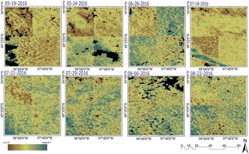
The black pixels of the high-resolution soil moisture maps presented in Figure 12 belong to the cloudy pixels, which were masked out using MODIS quality flags data generated at 1-km based on the visible and infrared channel data. For those pixels, it is not possible to estimate the SMC values due to the lack of LST measurements.

As Figure 12 indicates, some of the 1-km SMC maps contain the 36-km boxy artifact, which describes the coarse-scale grid that remains apparent in the downscaled maps. With the argument that an efficient disaggregation algorithm is able to spatially connect high-resolution disaggregated values between neighboring low-resolution pixels and remain less apparent the low-resolution boxes, Agam et al. (2007) introduced the notion of “boxy artifact” as a factor of the quality of disaggregation approaches (Duan and Li 2016; Oiha et al. 2018). According to (Agam et al. 2007), the less boxy artifact in the disaggregated maps, the better the disaggregation skill of the algorithm. As can be seen in Figure 12, for top row high-resolution maps, the spatial structures are less visible and the boxy artifact is more apparent. Although this effect is a common error in the disaggregation techniques, it threatens the accuracy of the high-resolution SMC maps (Oiha et al. 2018).

In order to an in-deep evaluation of the proposed method, we performed a spatial correlation analysis between estimated SMC values and their corresponding in situ measurements for 8 days in which all three in situ, SMAP, and MODIS data are available. The results are reported in Figure 13. Each point of Figure 13 represents an image pixel in which there was at least one in situ station. In addition, the measurements of those stations, which are located in one pixel, were averaged and then considered as ground truth.

Figure 13. SMC values extracted from the 1-year scatter plot concerning the corresponding in situ SMC measurements. Each point represents an image pixel in which there is at least one in situ station

According to Figure 13, there is a correlation coefficient of 0.66 between the field SMC measurements and estimated SMC values retrieved by the proposed method. Since the correlation coefficient between coarse-scale SMAP values and in situ measurements is 0.64 for SMAPVEX16 (see Table 2), achieving the results of Figure 13 is not out of expectation.

Moreover, Figure 13 also shows the bias of −0.03 and RMSE of 0.07 m³/m³ for the proposed method in estimating SMC values. With comparison to Table 2, one can see that coarse-scale SMAP data have RMSE and bias equal to 0.09 m³/m³ and 0.01 for SMAPVEX16 site. It means that the proposed method can disaggregate the low-resolution space-based microwave SMC products using proposed high-resolution SMC indices while at the same time, measurement accuracy is not lost but improved in all cases of our study. It must be mentioned that alongside coarse-scale passive SMC products, there are other products retrieved using a combination of active and passive MW technology (Entekhabi et al. 2010). In these kinds of products, the SMC values are measured, estimated, or simulated using the thermal emission and backscattering coefficient of soil retrieved from passive and active sensors, respectively. SMC retrieved from Sentinel-1 backscattering data (Alexakis et al. 2017), ASCAT SMC products (Kim et al. 2018), and SMAP 9 km soil moisture products interpolated and simulated using radar backscattering measurements (Das et al. 2018), are some examples of these data. Active-passive products have better spatial resolution than passive microwave products due to the high spatial resolution of radar sensors (Sabaghy et al. 2020). It cannot be said for sure that the accuracy of these products is globally more than the accuracy of SMAP soil moisture measurements and may even be less in some study areas (Kim et al. 2018; Chen et al. 2018; El Hajj et al. 2018; Mousa and Shu 2020). Better spatial resolution of active-passive SMC products makes them suitable options for application in downscaling algorithms, instead of passive SM_MW. However, applying radar-related measurements puts some essential theoretical changes in the proposed method. For example, in this case, the soil roughness parameters and the vegetation fraction, which are two effective parameters in the accuracy of radar backscattering measurement, should be modeled. Investigating the performance of active-passive SMC products along with long-term soil moisture indices extracted from the T-V scatter plot to retrieve SMC values at fine spatial and temporal resolution requires a very comprehensive study that we recommend for future researches.

Despite reaching a significant positive correlation between obtained and measured SMC values, the accuracy of the proposed method is threatened by some uncertainty resources, among which the most serious ones are, perhaps, as follows:

1. Depending on the SMC, optical/thermal frequencies and L-band frequencies have different penetration depths. Briefly, the penetration of the microwave portion of the electromagnetic spectrum increases from 5 cm to 1 m with decreasing the SMC value. It means that unlike the optical/thermal sensors that always measure the values from the surface, microwave remote sensing sensors have various penetration depths and measures the moisture content at different layers. This situation creates an uncertainty source due to the non-meaningful relationship between the amounts of water in the soil at a deeper layer and surface SMC. To clarify this issue, Figure 14 attempts to provide confirmatory evidence of the vertical inhomogeneity of soil moisture using spatial correlation analyses between the SMC values at different soil depths.

Figure 14. Correlation analysis between 5 cm soil moisture and the SMC of soil at depth (a) 20 cm, (b) 50 cm, and (c) 1 m

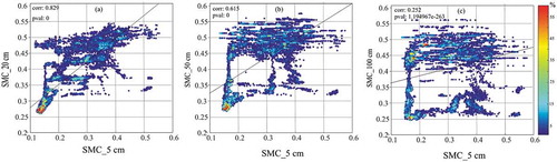
In Figure 14, the horizontal axes stand for the in situ SMC at 5 cm of soil measured by one of the RISMA stations, during 2016. Also, the vertical axes are the corresponding measurements at a depth of 20 cm (a), 50 cm (b), and 1 m (c). The scatter plots of Figure 14 provide confirmatory evidence that by increasing the depth of the soil, the relationship between measured SMC and soil surface SMC is diminished. This issue, which can be considered as a systematic error, is one of the primary uncertainty sources of our proposed method.

• (2)In dense vegetation cover and forested areas, the indices derived from the optical and thermal frequencies are less sensitive to the soil parameters, due to the less penetration. L-band frequencies, by contrast, can penetrate through even greater amounts of vegetation. It means that in dense vegetation conditions, the observations of microwave satellite and optical/thermal sensors are not necessarily obtained the same objects of the land surface. This can be one of the uncertainty sources in estimating high-resolution SMC maps.

• (3)The time lag between microwave and optical/thermal satellite images generally compiles a systematic error in our proposed algorithm. This is even more aggravated in cases of raining during two corresponding measurement times (such as 6 a.m. and 10:30 a.m. in daytime overpass).

• (4)The RFI would seem to be another uncertainty source of our proposed method. Although the SMAP mission is the less sensitive to the RFI, however, the effects of undetected ground-based surveillance radars can still contaminate the SMAP measurements, spastically where those effects are too small to detect and mitigate.

• (5)Our proposed method is developed on MODIS products. These products are already corrected for atmospheric effects. This point is in line with many current kinds of literature, such as Merlin et al. (2012), Wan (2014), and Zhou et al. (2014). In light of the atmospheric correction of MODIS products, we had satisfactory results in our previous methodology. However, daily variations in the climate conditions and its non-modeling effects may increase the uncertainty of the indices extracted from 1-year T-V scatter plot.

Conclusion

Over the past decade, there has been a dramatic increase in the number of studies that have focused on remote sensing techniques to retrieve soil moisture information. Among those techniques, the T-V scatter plot methods received particular attention due to their simple implementation and easy accessibility of the required data.

The purpose of this study was to develop T-V scatter plot methods in three aspects, including (1) improve its accuracy in cases that the scatter plot is not comprehensively formed, (2) make it capable to obtain the absolute soil moisture values, and (3) address the incompatibility of T-V soil moisture index maps of different days.

As the first step of the proposed method, space-based microwave soil moisture products of AMSR2, SMOS, and SMAP missions were validated via eight in situ soil moisture measurement networks over 5 years. As the next step, the T-V scatter plot method was used to obtain a high-resolution SMC index. In light of the premise that in long-term intervals more comprehensive humidity and vegetation situations are likely to happen, this study applied the 1-year T-V scatter plot. In consideration of the fact that those points related to extreme dry and wet days are likely to locate close to the annual dry and wet edges of the T-V scatter plot, we introduced a novel annual soil moisture index (called ASMI_HR) that proved to be in great consistency with ground-based soil moisture data. Using the annual soil moisture index ASMI_HR, along with microwave coarse-scale SMC products, we managed to introduce a novel temporal method for obtaining the parameter ∂SM_MW/∂SMI_HR, as one of the essential parameters in DisPATCh algorithm. Another achievement of this study was a daily SMC index (DSMI_HR) that is grounded on a novel concept of “co-moisture line” in the T-V scatter plot. Co-moisture lines were considered as a replacement of daily dry and wet edges allowing to apply the T-V scatter plot method in all days, even those with incomprehensive data to provide reliable daily dry and wet edges. In the last step of the proposed method, DSMI_HR was converted to the absolute SMC values using the DisPATCh algorithm.

The performance of the proposed method of this study was evaluated in each step. As mentioned before, in the first step, we evaluated the accuracy of microwave coarse-scale SMC measurements. It was found that the SMAP, with the averages of R = 0.73, RMSE = 0.07, bias = 0.02, and ubRMSE = 0.06, provides the most appropriate products for SMC retrieval (Figures 6 and 7 and Table 2). In the second step, we show an excellent consistency between the ASMI_HR index derived from the 1-year scatter plot and in situ SMC measurements (R = 0.65) using Figure 8. In this step, we also explain that how the annual SMC index extracted from 1-year scatter plot makes it possible to compare the SMC index maps of different days (Figure 9). As the last assessment of the proposed method, we evaluated the SMC values calculated using the proposed method with in situ measurements (Figure 13). The result shows an excellent consistency correlation coefficient of 0.66 and ubRMSE of 0.06 between the field SMC measurements and estimated SMC values are promising enough for most practical applications.

Despite the good performance of our proposed method in retrieving SMC information, the current method is only applicable in cloud-free conditions. Besides, the proposed method suffers from some uncertainty resources. For example, optical/thermal frequencies and L-band frequencies have different penetration depths, which causes a systematic error in our proposed method. In further studies, the influence of the depth of the soil on the SMC values extracted from microwave products, which is detected in this study, could be modeled and eliminated. Moreover, we applied the optical/thermal SMC indices extracted from T/V scatter plot, while some other optical/thermal SMC indices can be measured using long-term data and then applied to downscale passive coarse-scale measurements. The performance of various long-term optical/thermal indices in this proposed method can also be the object of further studies.

Highlights

• The problems of the T-V method in determining SM index are proved.

• Two adopted T-V indices are proposed.

• DisPATCh is employed as a downscaling algorithm to disaggregate the SMAP products.

• RTwo different T-V SM indices are simultaneously applied in the DisPATCh algorithm.

• Partial derivative parameter of the DisPATCh algorithm is developed.

References

- Abbaszadeh, P., H. Moradkhani, and X. Zhan. 2019. “Downscaling SMAP Radiometer Soil Moisture over the CONUS Using an Ensemble Learning Method.” Water Resources Research 55 (1): 324–344. doi:10.1029/2018WR023354.
- Agam, N., W. P. Kustas, M. C. Anderson, F. Li, and C. M. Neale. 2007. “A Vegetation Index Based Technique for Spatial Sharpening of Thermal Imagery.” Remote Sensing of Environment 107 (4): 545–558. doi:10.1016/j.rse.2006.10.006.
- Alexakis, D. D., F.-D. K. Mexis, A.-E. K. Vozinaki, I. N. Daliakopoulos, and I. K. Tsanis. 2017. “Soil Moisture Content Estimation Based on Sentinel-1 and Auxiliary Earth Observation Products. A Hydrological Approach.” Sensors 17: 1455.
- Al-yaari, A., J. P. Wigneron, A. Ducharne, Y. Kerr, D. E. Rosnay, P. De Jeu, R. Govind, et al. 2014. “Global-scale Evaluation of Two Satellite-based Passive Microwave Soil Moisture Datasets (SMOS and AMSR-E) with respect to Land Data Assimilation System Estimates.” Remote Sensing of Environment 149: 181–195. doi:10.1016/j.rse.2014.04.006.
- Bhuiyan, H. A., H. Mcnairn, J. Powers, M. Friesen, A. Pacheco, T. J. Jackson, M. H. Cosh, A. Colliander, A. Berg, and T. Rowlandson. 2018. “Assessing SMAP Soil Moisture Scaling and Retrieval in the Carman (Canada) Study Site.” Vadose Zone Journal 17 (1): 1–14.
- Bircher, S., N. Skou, K. H. Jensen, J. P. Walker, and L. Rasmussen. 2012. “A Soil Moisture and Temperature Network for SMOS Validation in Western Denmark.” Hydrology and Earth System Sciences 16 (5): 1445–1463. doi:10.5194/hess-16-1445-2012.
- Carlson, T. 2007. “An Overview of The” Triangle Method” for Estimating Surface Evapotranspiration and Soil Moisture from Satellite Imagery.” Sensors 7 (8): 1612–1629. doi:10.3390/s7081612.
- Carlson, T. N., R. R. Gillies, and E. M. Perry. 1994. “A Method to Make Use of Thermal Infrared Temperature and NDVI Measurements to Infer Surface Soil Water Content and Fractional Vegetation Cover.” Remote Sensing Reviews 9 (1–2): 161–173. doi:10.1080/02757259409532220.
- Carlson, T. N., R. R. Gillies, and T. J. Schmugge. 1995. “An Interpretation of Methodologies for Indirect Measurement of Soil Water Content.” Agricultural and Forest Meteorology 77 (3–4): 191–205. doi:10.1016/0168-1923(95)02261-U.
- Chan, S. K., R. Bindlish, P. E. O'Neill, E. Njoku, T. Jackson, A. Colliander, F. Chen et al. 2016. “Assessment of the SMAP passive soil moisture product.” IEEE Transactions on Geoscience and Remote Sensing 54 (8): 4994–5007.
- Chen, F., W. T. Crow, R. Bindlish, A. Colliander, M. S. Burgin, J. Asanuma, and K. Aida. 2018. “Global-scale Evaluation of SMAP, SMOS and ASCAT Soil Moisture Products Using Triple Collocation.” Remote Sensing of Environment 214: 1–13. doi:10.1016/j.rse.2018.05.008.
- Chen, Y., H. Sun, and J. Li. 2016. “Estimating Daily Maximum Air Temperature with MODIS Data and a Daytime Temperature Variation Model in Beijing Urban Area.” Remote Sensing Letters 7 (9): 865–874. doi:10.1080/2150704X.2016.1193792.
- Colliander, A., M. H. Cosh, S. Misra, T. J. Jackson, W. T. Crow, J. Powers, H. Mcnairn, P. Bullock, A. Berg, and R. Magagi. 2019. “Comparison of High-resolution Airborne Soil Moisture Retrievals to SMAP Soil Moisture during the SMAP Validation Experiment 2016 (SMAPVEX16).” Remote Sensing of Environment 227: 137–150. doi:10.1016/j.rse.2019.04.004.
- Colliander, A., T. J. Jackson, R. Bindlish, S. Chan, N. Das, S. Kim, M. Cosh, R. Dunbar, L. Dang, and L. Pashaian. 2017. “Validation of SMAP Surface Soil Moisture Products with Core Validation Sites.” Remote Sensing of Environment 191: 215–231. doi:10.1016/j.rse.2017.01.021.
- Cui, C., J. Xu, J. Zeng, K.-S. Chen, X. Bai, H. Lu, Q. Chen, and T. Zhao. 2018. “Soil Moisture Mapping from Satellites: An Intercomparison of SMAP, SMOS, FY3B, AMSR2, and ESA CCI over Two Dense Network Regions at Different Spatial Scales.” Remote Sensing 10 (2): 33. doi:10.3390/rs10010033.
- Cui, H., L. Jiang, J. Du, S. Zhao, G. Wang, Z. Lu, and J. Wang. 2017.“Evaluation and analysis of AMSR‐2, SMOS, and SMAP soil moisture products in the Genhe area of China.” Journal of Geophysical Research: Atmospheres 122 (6): 8650–8666.
- Das, N. N., D. Entekhabi, R. S. Dunbar, A. Colliander, F. Chen, W. Crow, T. J. Jackson, A. Berg, D. D. Bosch, and T. Caldwell. 2018. “The SMAP Mission Combined Active-passive Soil Moisture Product at 9 Km and 3 Km Spatial Resolutions.” Remote Sensing of Environment 211: 204–217. doi:10.1016/j.rse.2018.04.011.
- Dey, S., D. Mandal, V. Kumar, B. Banerjee, J. M. Lopez-sanchez, H. Mcnairn, and A. Bhattacharya. 2019. “Crop Phenology Classification Using A Representation Learning Network From Sentinel-1 SAR Data.” In IGARSS 2019-2019 IEEE International Geoscience and Remote Sensing Symposium, IEEE, 7184–7187.
- Djamai, N., R. Magagi, K. Goïta, O. Merlin, Y. Kerr, and A. Roy. 2016. “A Combination of DISPATCH Downscaling Algorithm with CLASS Land Surface Scheme for Soil Moisture Estimation at Fine Scale during Cloudy Days.” Remote Sensing of Environment 184: 1–14. doi:10.1016/j.rse.2016.06.010.
- Dorigo, W., A. Gruber, R. De Jeu, W. Wagner, T. Stacke, A. Loew, C. Albergel, L. Brocca, D. Chung, and R. Parinussa. 2015. “Evaluation of the ESA CCI Soil Moisture Product Using Ground-based Observations.” Remote Sensing of Environment 162: 380–395. doi:10.1016/j.rse.2014.07.023.
- Duan, S.-B., and Z.-L. Li. 2016. “Spatial Downscaling of MODIS Land Surface Temperatures Using Geographically Weighted Regression: Case Study in Northern China.” IEEE Transactions on Geoscience and Remote Sensing 54 (11): 6458–6469. doi:10.1109/TGRS.2016.2585198.
- El Hajj, M., N. Baghdadi, M. Zribi, N. Rodríguez-fernández, J. P. Wigneron, A. Al-yaari, A. Al Bitar, C. Albergel, and J.-C. Calvet. 2018. “Evaluation of SMOS, SMAP, ASCAT and Sentinel-1 Soil Moisture Products at Sites in Southwestern France.” Remote Sensing 10 (4): 569. doi:10.3390/rs10040569.
- Entekhabi, D., E. G. Njoku, P. E. O’neill, K. H. Kellogg, W. T. Crow, W. N. Edelstein, J. K. Entin, S. D. Goodman, T. J. Jackson, and J. Johnson. 2010. The Soil Moisture Active Passive (SMAP) Mission. Proceedings of the IEEE, 98 (5): 704–716.
- Entekhabi, D., N. Das, E. Njoku, J. Johnson, and J. Shi. 2014. Algorithm Theoretical Basis Document L2 & L3 Radar/radiometer Soil Moisture (Active/passive) Data Products. Pasadena, CA, USA: Jet Propulsion Laboratory, California Institute of Technology.
- Fang, B., V. Lakshmi, R. Bindlish, T. J. Jackson, M. Cosh, and J. Basara. 2013. “Passive Microwave Soil Moisture Downscaling Using Vegetation Index and Skin Surface Temperature.” Vadose Zone Journal 12 (3): 1–19.
- Ford, T. W., and S. M. Quiring. 2019. “Comparison of Contemporary in Situ, Model, and Satellite Remote Sensing Soil Moisture with a Focus on Drought Monitoring.” Water Resources Research 55 (2): 1565–1582. doi:10.1029/2018WR024039.
- Garcia, M., N. Fernández, L. Villagarcía, F. Domingo, J. Puigdefábregas, and I. Sandholt. 2014. “Accuracy of the Temperature–Vegetation Dryness Index Using MODIS under Water-limited Vs. Energy-limited Evapotranspiration Conditions.” Remote Sensing of Environment 149: 100–117. doi:10.1016/j.rse.2014.04.002.
- Ghahremanloo, M., M. R. Mobasheri, and M. Amani. 2019. “Soil Moisture Estimation Using Land Surface Temperature and Soil Temperature at 5 Cm Depth.” International Journal of Remote Sensing 40 (1): 104–117. doi:10.1080/01431161.2018.1501167.
- Gillies, R., W. Kustas, and K. Humes. 1997. “A Verification of The’triangle’method for Obtaining Surface Soil Water Content and Energy Fluxes from Remote Measurements of the Normalized Difference Vegetation Index (NDVI) and Surface E.” International Journal of Remote Sensing 18 (15): 3145–3166. doi:10.1080/014311697217026.
- Grant, J. P., J. P. Wigneron, R. A. M. De Jeu, H. Lawrence, A. Mialon, P. Richaume, A. Al Bitar, M. Drusch, M. J. E. Van Marle, and Y. Kerr. 2016. “Comparison of SMOS and AMSR-E vegetation optical depth to four MODIS-based vegetation indices”. Remote Sensing of Environment 172: 87–100.
- He, L., Y. Hong, X. Wu, N. Ye, J. P. Walker, and X. Chen. 2018. “Investigation of SMAP Active–Passive Downscaling Algorithms Using Combined Sentinel-1 SAR and SMAP Radiometer Data.” IEEE Transactions on Geoscience and Remote Sensing 56 (8): 4906–4918. doi:10.1109/TGRS.2018.2842153.
- Hornbuckle, B., V. Walker, B. Eichinger, V. Wallace, and E. Yildirim Soil Surface Roughness Observed during SMAPVEX16-IA and Its Potential Consequences for SMOS and SMAP. 2017 IEEE International Geoscience and Remote Sensing Symposium (IGARSS), 2017. IEEE, 2027–2030.
- Jackson, T. J., M. H. Cosh, R. Bindlish, P. J. Starks, D. D. Bosch, M. Seyfried, D. C. Goodrich, M. S. Moran, and J. Du. 2010. “Validation of Advanced Microwave Scanning Radiometer Soil Moisture Products.” IEEE Transactions on Geoscience and Remote Sensing 48 (12): 4256–4272. doi:10.1109/TGRS.2010.2051035.
- Kerr, Y. H., A. Al-yaari, N. Rodriguez-fernandez, M. Parrens, B. Molero, D. Leroux, S. Bircher, A. Mahmoodi, A. Mialon, and P. Richaume. 2016a. “Overview of SMOS Performance in Terms of Global Soil Moisture Monitoring after Six Years in Operation.” Remote Sensing of Environment 180: 40–63. doi:10.1016/j.rse.2016.02.042.
- Kerr, Y. H., P. Waldteufel, J.-P. Wigneron, J. Martinuzzi, J. Font, and M. Berger. 2001. “Soil Moisture Retrieval from Space: The Soil Moisture and Ocean Salinity (SMOS) Mission.” IEEE Transactions on Geoscience and Remote Sensing 39 (8): 1729–1735. doi:10.1109/36.942551.
- Kerr, Y. H., P. Waldteufel, J.-P. Wigneron, S. Delwart, F. Cabot, J. Boutin, M.-J. Escorihuela, J. Font, N. Reul, and C. Gruhier 2010. The SMOS Mission: New Tool for Monitoring Key Elements Ofthe Global Water Cycle. Proceedings of the IEEE, 98, 666–687.
- Kim, H., R. Parinussa, A. G. Konings, W. Wagner, M. H. Cosh, V. Lakshmi, M. Zohaib, and M. Choi. 2018. “Global-scale Assessment and Combination of SMAP with ASCAT (Active) and AMSR2 (Passive) Soil Moisture Products.” Remote Sensing of Environment 204: 260–275. doi:10.1016/j.rse.2017.10.026.
- Kim, S., K. Balakrishnan, Y. Liu, F. Johnson, and A. Sharma. 2017. “Spatial Disaggregation of Coarse Soil Moisture Data by Using High-resolution Remotely Sensed Vegetation Products.” IEEE Geoscience and Remote Sensing Letters 14 (9): 1604–1608. doi:10.1109/LGRS.2017.2725945.
- Kim, S., Y. Y. Liu, F. M. Johnson, R. M. Parinussa, and A. Sharma. 2015. “A Global Comparison of Alternate AMSR2 Soil Moisture Products: Why Do They Differ?” Remote Sensing of Environment 161: 43–62. doi:10.1016/j.rse.2015.02.002.
- Kolassa, J., R. Reichle, Q. Liu, S. Alemohammad, P. Gentine, K. Aida, J. Asanuma, S. Bircher, T. Caldwell, and A. Colliander. 2018. “Estimating Surface Soil Moisture from SMAP Observations Using a Neural Network Technique.” Remote Sensing of Environment 204: 43–59. doi:10.1016/j.rse.2017.10.045.
- Kumar, S. V., P. A. Dirmeyer, C. D. Peters-lidard, R. Bindlish, and J. Bolten. 2018. “Information Theoretic Evaluation of Satellite Soil Moisture Retrievals.” Remote Sensing of Environment 204: 392–400. doi:10.1016/j.rse.2017.10.016.
- Lambin, E. F., and D. Ehrlich. 1996. “The Surface Temperature-vegetation Index Space for Land Cover and Land-cover Change Analysis.” International Journal of Remote Sensing 17 (3): 463–487. doi:10.1080/01431169608949021.
- Liu, L., J. Liao, X. Chen, G. Zhou, Y. Su, Z. Xiang, Z. Wang, X. Liu, Y. Li, and J. Wu. 2017. “The Microwave Temperature Vegetation Drought Index (MTVDI) Based on AMSR-E Brightness Temperatures for Long-term Drought Assessment across China (2003–2010).” Remote Sensing of Environment 199: 302–320. doi:10.1016/j.rse.2017.07.012.
- Liu, Y., and H. Yue. 2018. “The Temperature Vegetation Dryness Index (TVDI) Based on Bi-parabolic NDVI-Ts Space and Gradient-based Structural Similarity (GSSIM) for Long-term Drought Assessment across Shaanxi Province, China (2000–2016).” Remote Sensing 10 (6): 959. doi:10.3390/rs10060959.
- Long, D., V. P. Singh, and B. R. Scanlon. 2012. “Deriving Theoretical Boundaries to Address Scale Dependencies of Triangle Models for Evapotranspiration Estimation.” Journal of Geophysical Research: Atmospheres 117 (D5).
- Ma, H., J. Zeng, N. Chen, X. Zhang, M. H. Cosh, and W. Wang. 2019. “Satellite surface soil moisture from SMAP, SMOS, AMSR2 and ESA CCI: A comprehensive assessment using global ground-based observations.” Remote Sensing of Environment 231: 111215.
- Malbéteau, Y., O. Merlin, B. Molero, C. Rüdiger, and S. Bacon. 2016. “DisPATCh as a Tool to Evaluate Coarse-scale Remotely Sensed Soil Moisture Using Localized in Situ Measurements: Application to SMOS and AMSR-E Data in Southeastern Australia.” International Journal of Applied Earth Observation and Geoinformation 45: 221–234. doi:10.1016/j.jag.2015.10.002.
- Mallick, K., B. K. Bhattacharya, and N. Patel. 2009. “Estimating Volumetric Surface Moisture Content for Cropped Soils Using a Soil Wetness Index Based on Surface Temperature and NDVI.” Agricultural and Forest Meteorology 149 (8): 1327–1342. doi:10.1016/j.agrformet.2009.03.004.
- Mcnairn, H., T. J. Jackson, G. Wiseman, S. Belair, A. Berg, P. Bullock, A. Colliander, M. H. Cosh, S.-B. Kim, and R. Magagi. 2015. “The Soil Moisture Active Passive Validation Experiment 2012 (SMAPVEX12): Prelaunch Calibration and Validation of the SMAP Soil Moisture Algorithms.” IEEE Transactions on Geoscience and Remote Sensing 53 (5): 2784–2801. doi:10.1109/TGRS.2014.2364913.
- Merlin, O., B. Duchemin, O. Hagolle, F. Jacob, B. Coudert, G. Chehbouni, G. Dedieu, J. Garatuza, and Y. Kerr. 2010. “Disaggregation of MODIS Surface Temperature over an Agricultural Area Using a Time Series of Formosat-2 Images.” Remote Sensing of Environment 114 (11): 2500–2512. doi:10.1016/j.rse.2010.05.025.
- Merlin, O., C. Rudiger, A. Al Bitar, P. Richaume, J. P. Walker, and Y. H. Kerr. 2012. “Disaggregation of SMOS Soil Moisture in Southeastern Australia.” IEEE Transactions on Geoscience and Remote Sensing 50 (5): 1556–1571. doi:10.1109/TGRS.2011.2175000.
- Merlin, O., J. P. Walker, A. Chehbouni, and Y. Kerr. 2008. “Towards Deterministic Downscaling of SMOS Soil Moisture Using MODIS Derived Soil Evaporative Efficiency.” Remote Sensing of Environment 112 (10): 3935–3946. doi:10.1016/j.rse.2008.06.012.
- Minacapilli, M., S. Consoli, D. Vanella, G. Ciraolo, and A. Motisi. 2016. “A Time Domain Triangle Method Approach to Estimate Actual Evapotranspiration: Application in A Mediterranean Region Using MODIS and MSG-SEVIRI Products.” Remote Sensing of Environment 174: 10–23. doi:10.1016/j.rse.2015.12.018.
- Mohseni, F., and M. Mokhtarzade. 2020. “A New Soil Moisture Index Driven from an Adapted Long-term Temperature-vegetation Scatter Plot Using MODIS Data.” Journal of Hydrology 581: 124420. doi:10.1016/j.jhydrol.2019.124420.
- Monteith, J. L. 1965. Evaporation and Environment. Symposia of the Society for Experimental Biology, 205–234. Cambridge: Cambridge University Press (CUP).
- Moran, M., T. Clarke, Y. Inoue, and A. Vidal. 1994. “Estimating Crop Water Deficit Using the Relation between Surface-air Temperature and Spectral Vegetation Index.” Remote Sensing of Environment 49 (3): 246–263. doi:10.1016/0034-4257(94)90020-5.
- Mousa, B., and H. Shu. 2020. “Spatial Evaluation and Assimilation of SMAP, SMOS, and ASCAT Satellite Soil Moisture Products over Africa Using Statistical Techniques.” Earth and Space Science 7 (1): e2019EA000841. doi:10.1029/2019EA000841.
- Nemani, R., L. Pierce, S. Running, and S. Goward. 1993. “Developing Satellite-derived Estimates of Surface Moisture Status.” Journal of Applied Meteorology 32 (3): 548–557. doi:10.1175/1520-0450(1993)032<0548:DSDEOS>2.0.CO;2.
- Neuhauser, M., S. Verrier, O. Merlin, B. Molero, C. Suere, and S. Mangiarotti. 2019. “Multi-scale Statistical Properties of Disaggregated SMOS Soil Moisture Products in Australia.” Advances in Water Resources 134: 103426. doi:10.1016/j.advwatres.2019.103426.
- Njoku, E. G., P. Ashcroft, T. K. Chan, and L. Li. 2005. “Global Survey and Statistics of Radio-frequency Interference in AMSR-E Land Observations.” IEEE Transactions on Geoscience and Remote Sensing 43 (5): 938–947. doi:10.1109/TGRS.2004.837507.
- O’neill, P., S. Chan, E. Njoku, T. Jackson, and R. Bindlish. 2017. Algorithm Theoretical Basis Document Level 2 & 3 Soil Moisture (Passive) Data Products; Revision B. Pasadena, CA, USA: Jet Propulsion Lab., California Inst. Technol.
- Oiha, N., O. Merlin, B. Molero, C. Sucre, L. Olivera, V. Rivalland, and S. Er-raki Sequential Downscaling of the SMOS Soil Moisture at 100 M Resolution via a Variable Intermediate Spatial Resolution. IGARSS 2018-2018 IEEE International Geoscience and Remote Sensing Symposium, 2018. IEEE, 3735–3738.
- Pacheco, A., J. L’heureux, H. Mcnairn, J. Powers, A. Howard, X. Geng, P. Rollin, K. Gottfried, J. Freeman, and R. Ojo. 2014. “Real‐time In‐situ Soil Monitoring for Agriculture (RISMA) Network Metadata.” Science and Technology.
- Patel, N., A. Mukund, and B. R. Parida. 2019. “Satellite-derived Vegetation Temperature Condition Index to Infer Root Zone Soil Moisture in Semi-arid Province of Rajasthan, India.” Geocarto International 1–17. doi:10.1080/10106049.2019.1704074.
- Peng, J., A. Loew, S. Zhang, J. Wang, and J. Niesel. 2015. “Spatial Downscaling of Satellite Soil Moisture Data Using a Vegetation Temperature Condition Index.” IEEE Transactions on Geoscience and Remote Sensing 54 (1): 558–566. doi:10.1109/TGRS.2015.2462074.
- Petropoulos, G., T. Carlson, M. Wooster, and S. Islam. 2009. “A Review of Ts/VI Remote Sensing Based Methods for the Retrieval of Land Surface Energy Fluxes and Soil Surface Moisture.” Progress in Physical Geography 33 (2): 224–250. doi:10.1177/0309133309338997.
- Petropoulos, G. P., G. Ireland, and B. Barrett. 2015. “Surface Soil Moisture Retrievals from Remote Sensing: Current Status, Products & Future Trends.” Physics and Chemistry of the Earth, Parts A/B/C 83: 36–56. doi:10.1016/j.pce.2015.02.009.
- Piles, M., A. Camps, M. Vall-llossera, I. Corbella, R. Panciera, C. Rudiger, Y. H. Kerr, and J. Walker. 2011. “Downscaling SMOS-Derived Soil Moisture Using MODIS Visible/Infrared Data.” IEEE Transactions on Geoscience and Remote Sensing 49 (9): 3156–3166. doi:10.1109/TGRS.2011.2120615.
- Przeździecki, K., and J. Zawadzki. 2020. “Modification of the Land Surface Temperature–Vegetation Index Triangle Method for Soil Moisture Condition Estimation by Using SYNOP Reports.” Ecological Indicators 119: 106823. doi:10.1016/j.ecolind.2020.106823.
- Rahimzadeh-bajgiran, P., A. A. Berg, C. Champagne, and K. Omasa. 2013. “Estimation of Soil Moisture Using Optical/thermal Infrared Remote Sensing in the Canadian Prairies.” ISPRS Journal of Photogrammetry and Remote Sensing 83: 94–103. doi:10.1016/j.isprsjprs.2013.06.004.
- Rahimzadeh-bajgiran, P., K. Omasa, and Y. Shimizu. 2012. “Comparative Evaluation of the Vegetation Dryness Index (VDI), the Temperature Vegetation Dryness Index (TVDI) and the Improved TVDI (Itvdi) for Water Stress Detection in Semi-arid Regions of Iran.” ISPRS Journal of Photogrammetry and Remote Sensing 68: 1–12. doi:10.1016/j.isprsjprs.2011.10.009.
- Rodríguez-fernández, N., A. Al Bitar, A. Colliander, and T. Zhao. 2019. Soil Moisture Remote Sensing across Scales (p. 190). Multidisciplinary Digital Publishing Institute.
- Rowlandson, T., S. Impera, J. Belanger, A. A. Berg, B. Toth, and R. Magagi. 2015. “Use of in Situ Soil Moisture Network for Estimating Regional-scale Soil Moisture during High Soil Moisture Conditions.” Canadian Water Resources Journal/Revue Canadienne Des Ressources Hydriques 40 (4): 343–351. doi:10.1080/07011784.2015.1061948.
- Sabaghy, S., J. P. Walker, L. J. Renzullo, R. Akbar, S. Chan, J. Chaubell, N. Das, R. S. Dunbar, D. Entekhabi, and A. Gevaert. 2020. “Comprehensive Analysis of Alternative Downscaled Soil Moisture Products.” Remote Sensing of Environment 239: 111586. doi:10.1016/j.rse.2019.111586.
- Saber, M., K. I. Abdrabo, O. M. Habiba, S. A. Kantosh, and T. Sumi. 2020. “Impacts of Triple Factors on Flash Flood Vulnerability in Egypt: Urban Growth, Extreme Climate, and Mismanagement.” Geosciences 10 (1): 24. doi:10.3390/geosciences10010024.
- Sadeghi, M., E. Babaeian, M. Tuller, and S. B. Jones. 2017. “The Optical Trapezoid Model: A Novel Approach to Remote Sensing of Soil Moisture Applied to Sentinel-2 and Landsat-8 Observations.” Remote Sensing of Environment 198: 52–68. doi:10.1016/j.rse.2017.05.041.
- Sánchez-ruiz, S., M. Piles, N. Sánchez, J. Martínez-fernández, M. Vall-llossera, and A. Camps. 2014. “Combining SMOS with Visible and Near/shortwave/thermal Infrared Satellite Data for High Resolution Soil Moisture Estimates.” Journal of Hydrology 516: 273–283. doi:10.1016/j.jhydrol.2013.12.047.
- Sandholt, I., K. Rasmussen, and J. Andersen. 2002. “A Simple Interpretation of the Surface Temperature/vegetation Index Space for Assessment of Surface Moisture Status.” Remote Sensing of Environment 79 (2–3): 213–224. doi:10.1016/S0034-4257(01)00274-7.
- Secord, A. Weighted Voronoi Stippling. Proceedings of the 2nd international symposium on Non-photorealistic animation and rendering, 2002. ACM, 37–43.
- Smith, A., J. P. Walker, A. W. Western, R. Young, K. Ellett, R. Pipunic, R. Grayson, L. Siriwardena, F. Chiew, and H. Richter. 2012. “The Murrumbidgee Soil Moisture Monitoring Network Data Set.” Water Resources Research 48 (7).
- Sun, H., B. Zhou, C. Zhang, H. Liu, and B. Yang. 2020. “DSCALE_mod16: A Model for Disaggregating Microwave Satellite Soil Moisture with Land Surface Evapotranspiration Products and Gridded Meteorological Data.” Remote Sensing 12 (6): 980. doi:10.3390/rs12060980.
- Sun, H., Y. Wang, W. Liu, S. Yuan, and R. Nie. 2017. “Comparison of Three Theoretical Methods for Determining Dry and Wet Edges of the LST/FVC Space: Revisit of Method Physics.” Remote Sensing 9: 528.
- Tang, R., Z.-L. Li, and B. Tang. 2010. “An Application of the Ts–VI Triangle Method with Enhanced Edges Determination for Evapotranspiration Estimation from MODIS Data in Arid and Semi-arid Regions: Implementation and Validation.” Remote Sensing of Environment 114 (3): 540–551. doi:10.1016/j.rse.2009.10.012.
- Tavakol, A., V. Rahmani, S. M. Quiring, and S. V. Kumar. 2019. “Evaluation Analysis of NASA SMAP L3 and L4 and SPoRT-LIS Soil Moisture Data in the United States.” Remote Sensing of Environment 229: 234–246. doi:10.1016/j.rse.2019.05.006.
- Tetlock, E., B. Toth, A. Berg, T. Rowlandson, and J. T. Ambadan. 2019. “An 11-year (2007–2017) Soil Moisture and Precipitation Dataset from the Kenaston Network in the Brightwater Creek Basin, Saskatchewan, Canada.” Earth System Science Data 11 (2): 787–796. doi:10.5194/essd-11-787-2019.
- Vani, V., K. Pavan Kumar, and M. V. Ravibabu. 2019. “Temperature and Vegetation Indices Based Surface Soil Moisture Estimation: A Remote Sensing Data Approach.” In Proceedings of international conference on remote sensing for disaster management, pp. 281–289. Springer, Cham.
- Wan, Z. 2014. “New Refinements and Validation of the Collection-6 MODIS Land-surface Temperature/emissivity Product.” Remote Sensing of Environment 140: 36–45. doi:10.1016/j.rse.2013.08.027.
- Wang, L., and J. J. Qu. 2009. “Satellite Remote Sensing Applications for Surface Soil Moisture Monitoring: A Review.” Frontiers of Earth Science in China 3 (2): 237–247. doi:10.1007/s11707-009-0023-7.
- Wang, P.-X., X.-W. Li, J.-Y. Gong, and C. Song Vegetation Temperature Condition Index and Its Application for Drought Monitoring. IGARSS 2001. Scanning the Present and Resolving the Future. Proceedings. IEEE 2001 International Geoscience and Remote Sensing Symposium (Cat. No. 01CH37217), 2001. IEEE, 141–143.
- Wang, S., M. Garcia, A. Ibrom, J. Jakobsen, C. Josef Köppl, K. Mallick, M. Looms, and P. Bauer-gottwein. 2018. “Mapping Root-Zone Soil Moisture Using a Temperature–Vegetation Triangle Approach with an Unmanned Aerial System: Incorporating Surface Roughness from Structure from Motion.” Remote Sensing 10 (12): 1978. doi:10.3390/rs10121978.
- Wen, X., H. Lu, C. Li, T. Koike, and I. Kaihotsu. 2014. “Inter-comparison of soil moisture products from SMOS, AMSR-E, ECWMF and GLDAS over the Mongolia Plateau.” In Land Surface Remote Sensing II 9260: 92600O. International Society for Optics and Photonics.
- Yang, J., and D. Zhang. 2019. “Soil Moisture Estimation with a Remotely Sensed Dry Edge Determination Based on the Land Surface Temperature-vegetation Index Method.” Journal of Applied Remote Sensing 13 (2): 024511. doi:10.1117/1.JRS.13.024511.
- Yang, K., J. Qin, L. Zhao, Y. Chen, W. Tang, M. Han, Z. Chen, N. Lv, B. Ding, and H. Wu. 2013. “A Multiscale Soil Moisture and Freeze–thaw Monitoring Network on the Third Pole.” Bulletin of the American Meteorological Society 94 (12): 1907–1916. doi:10.1175/BAMS-D-12-00203.1.
- Yang, Y., H. Guan, D. Long, B. Liu, G. Qin, J. Qin, and O. Batelaan. 2015. “Estimation of Surface Soil Moisture from Thermal Infrared Remote Sensing Using an Improved Trapezoid Method.” Remote Sensing 7 (7): 8250–8270. doi:10.3390/rs70708250.
- Yee, M. S., J. P. Walker, C. Rüdiger, R. M. Parinussa, T. Koike, and Y. H. Kerr. 2017. “A comparison of SMOS and AMSR2 soil moisture using representative sites of the OzNet monitoring network.” Remote Sensing of Environment 195: 297–312.
- Zhang, D., and G. Zhou. 2016. “Estimation of Soil Moisture from Optical and Thermal Remote Sensing: A Review.” Sensors 16 (8): 1308. doi:10.3390/s16081308.
- Zhang, D., R. Tang, W. Zhao, B. Tang, H. Wu, K. Shao, and Z.-L. Li. 2014. “Surface Soil Water Content Estimation from Thermal Remote Sensing Based on the Temporal Variation of Land Surface Temperature.” Remote Sensing 6 (4): 3170–3187. doi:10.3390/rs6043170.
- Zhang, R., J. Tian, H. Su, X. Sun, S. Chen, and J. Xia. 2008. “Two Improvements of an Operational Two-layer Model for Terrestrial Surface Heat Flux Retrieval.” Sensors 8 (10): 6165–6187. doi:10.3390/s8106165.
- Zhang, R., S. Kim, and A. Sharma. 2019. “A Comprehensive Validation of the SMAP Enhanced Level-3 Soil Moisture Product Using Ground Measurements over Varied Climates and Landscapes.” Remote Sensing of Environment 223: 82–94. doi:10.1016/j.rse.2019.01.015.
- Zhao, W., N. Sánchez, H. Lu, and A. Li. 2018. “A Spatial Downscaling Approach for the SMAP Passive Surface Soil Moisture Product Using Random Forest Regression.” Journal of Hydrology 563: 1009–1024. doi:10.1016/j.jhydrol.2018.06.081.
- Zhou, J., X. Zhang, W. Zhan, and H. Zhang. 2014. “Land Surface Temperature Retrieval from MODIS Data by Integrating Regression Models and the Genetic Algorithm in an Arid Region.” Remote Sensing 6 (6): 5344–5367. doi:10.3390/rs6065344.
- Zhu, W., A. Lv, S. Jia, and L. Sun. 2017b. “Development and Evaluation of the MTVDI for Soil Moisture Monitoring.” Journal of Geophysical Research: Atmospheres 122: 5533–5555.
- Zhu, W., S. Jia, and A. Lv. 2017a. “A Time Domain Solution of the Modified Temperature Vegetation Dryness Index (MTVDI) for Continuous Soil Moisture Monitoring.” Remote Sensing of Environment 200: 1–17. doi:10.1016/j.rse.2017.07.032.