A comparative analysis of trajectory similarity measures

ABSTRACT

Computing trajectory similarity is a fundamental operation in movement analytics, required in search, clustering, and classification of trajectories, for example. Yet the range of different but interrelated trajectory similarity measures can be bewildering for researchers and practitioners alike. This paper describes a systematic comparison and methodical exploration of trajectory similarity measures. Specifically, this paper compares five of the most important and commonly used similarity measures: dynamic time warping (DTW), edit distance (EDR), longest common subsequence (LCSS), discrete Fréchet distance (DFD), and Fréchet distance (FD). The paper begins with a thorough conceptual and theoretical comparison. This comparison highlights the similarities and differences between measures in connection with six different characteristics, including their handling of a relative versus absolute time and space, tolerance to outliers, and computational efficiency. The paper further reports on an empirical evaluation of similarity in trajectories with contrasting properties: data about constrained bus movements in a transportation network, and the unconstrained movements of wading birds in a coastal environment. A set of four experiments: a. creates a measurement baseline by comparing similarity measures to a single trajectory subjected to various transformations; b. explores the behavior of similarity measures on network-constrained bus trajectories, grouped based on spatial and on temporal similarity; c. assesses similarity with respect to known behavioral annotations (flight and foraging of oystercatchers); and d. compares bird and bus activity to examine whether they are distinguishable based solely on their movement patterns. The results show that in all instances both the absolute value and the ordering of similarity may be sensitive to the choice of measure. In general, all measures were more able to distinguish spatial differences in trajectories than temporal differences. The paper concludes with a high-level summary of advice and recommendations for selecting and using trajectory similarity measures in practice, with conclusions spanning our three complementary perspectives: conceptual, theoretical, and empirical.

KEYWORDS:

• Trajectory similarity
• movement analytics
• similarity measures
• network-constrained movement

Introduction

Trajectories – recording the evolving position of objects in geographic space and time – are fundamental building blocks of computational movement analysis (Laube 2014). Trajectories have become ubiquitous in a wide range of applications, from analysis at the scale of micro-organisms in laboratory settings in the environmental sciences (Nathan et al. 2008) to global-scale species migrations and interactions (Horne et al. 2007; Andersson et al. 2008). Trajectory analysis has been applied to the movement of “crisp” objects, such as the movement of birds, people, and vehicles (Fritz, Said, and Weimerskirch 2003; González, Hidalgo, and Albert-László 2008; Arslan, Cruz, and Ginhac 2019; Y. Liu et al. 2012), as well as ill-defined objects, such as hurricanes (Dodge, Laube, and Weibel 2012). Trajectory analysis has also been applied to “unconstrained” movements, such as movement of ships and aircraft (Kaluza, Andrea Kölzsch, and Blasius 2010; Varlamis et al. 2019), as well as movement within a transportation network, such as the movement of buses and cars (Tao, Both, and Duckham 2017; Gong et al. 2019).

Irrespective of these different settings, a fundamental operation for comparing two trajectories is the measurement of trajectory similarity. Measuring trajectory similarity is key to analysis tasks including search (find the most similar trajectory in a collection to a given trajectory, e.g. (Buchin et al. 2011)), clustering (group trajectories with similar properties, e.g. (Zhang, Huang, and Tan 2006)), classification (identifying trajectories associated with a known set of properties, e.g. (Bashir, Khokhar, and Schonfeld 2007)), and aggregation and characterization (identifying representative trajectories and their properties, e.g. (K. Buchin et al. 2013)).

In the context of this wide range of applications, a plethora of methods for measuring trajectory similarity has emerged in parallel, and sometimes in isolation, across diverse academic communities. These communities include (but are not limited to) geographic information science (Dodge, Laube, and Weibel 2012; Petry et al. 2019a), computational geometry (Buchin et al. 2011), knowledge discovery and databases (Pelekis et al. 2007), movement ecology (Demšar et al. 2015), and transport studies (Zhang et al. 2011).

Our aim in this paper is to explore trajectory similarity measures systematically and from three complementary perspectives: conceptual, theoretical, and empirical. More specifically, in this paper we:

• set out and explore a conceptual model of trajectory similarity, illustrated through a set of examples;

• populate our conceptual model with a set of algorithms and explore their theoretical properties from the perspective of computational geometry; and

• explore experimentally the different properties of selected algorithms through two contrasting data sets (constrained movement of vehicles on a network, and quasi-unconstrained movement of birds in a 2D space).

The analysis in this paper focuses on a representative subset of arguably the most well known and commonly used of measures: dynamic time warping (Berndt and Clifford 1994) (DTW), edit distance on real sequences (EDR) (Chen, Özsu, and Oria 2005), Longest common subsequence (LCSS)(Vlachos, Gunopulos, and Kollios 2002), Fréchet distance (FD) (Alt and Godau 1995) and its discrete counterpart, the discrete Fréchet distance (DFD) (Eiter and Mannila 1994). All of these measures are described further in detail in Section 4, with a full justification of their selection in Section 3 and following the review of the background literature in Section 2. The outcomes and conclusions of the work in Sections 7 and 8 aim to provide clear, useful, and generalizable recommendations for researchers and practitioners seeking to use trajectory similarity measures.

Background

To date, relatively few comparative studies have sought to reconnect the diverse communities that use trajectory similarity measures. Two welcome early exceptions in this regard include the work of (Magdy et al. 2015) and of (Wang et al. 2013), who explored in an empirical setting the effectiveness of a range of trajectory similarity measures. However, though the latter compared measures, their conclusions are based on a small number of trajectories in a constrained network space, and lack a theoretical underpinning. The former paper briefly characterizes trajectories conceptually, but lacks empirical examples.

Two more recent works also addressed the need to compare and analyze similarity measures for trajectories, in a spirit more similar to ours. (Cleasby et al. 2019) analyzed five different measures (four of which we also include) in order to understand how they compare to each other when applied to movement ecology. They carried out simulations with synthetic data and also included experiments with a real data set of northern gannet trajectories. The study was focused on ecology applications, but some of its conclusions are more broadly relevant too. The survey by (Su et al. 2020) provides a computational comparison of an impressive selection of 15 similarity measures. The authors evaluated how capable are these measures of handling different transformations to the data (e.g. adding/deleting points, changing sampling rate, etc.). However, the comparison among these similarity measures emphasizes the computational rather than conceptual perspective, for example, experimenting with synthetic data rather than real data.

Hence, our approach complements this work by (Cleasby et al. 2019; Su et al. 2020), by adopting a GI science perspective that balances the more application-specific and more computational perspectives of this related recent work. Based on this holistic approach, this paper aims to not only explore the properties of the different trajectory similarity algorithms and measures but also to characterize the different ways in which choice of algorithm and measure impacts on the results of analysis of real data.

Similarity measures and algorithms

Trajectory similarity measures have received considerable attention in several areas, with a large number of similarity measures proposed in the literature.

Perhaps the simplest approach to measure how similar two trajectories are is to measure spatial distance between corresponding locations (i.e. the first two points of each trajectory, the second two points, and so on). This is what we call lock-step Euclidean distance. From there on, measures attempt to compare locations in more sophisticated ways.

Several other similarity measures have been proposed, but most of them can be seen as extensions, generalizations, and improvements (e.g. in terms of computation time) of the basic measures mentioned above. For instance, sequence weighted alignment (SWALE) (Morse and Patel 2007) generalizes in a unified model EDR and LCSS. The edit distance with projections (EDwP) (Ranu et al. 2015) is a variant of EDR that uses projections to handle non-uniform sampling rates. The w-constrained discrete Fréchet distance (wDF) (Ding, Trajcevski, and Scheuermann 2008) is a variant of DFD where two points are matched only if their timestamps are within a given time distance. The uncertain movement similarity (UMS) (Furtado et al. 2018) replaces the fixed global threshold of the lock-step Euclidean distance by different ellipses that are used to associate points from both trajectories.

While many of the measures proposed above can be generalized to higher-dimensional data, some have been adapted specifically to this setting, such as DTW for multi-dimensional time series (MD-DTW) (Holt Ten, Reinders, and Hendriks 2007). A particularly important case of multidimensional trajectories are semantic trajectories (Spaccapietra et al. 2008). These are trajectories that are enriched with additional semantic information.

Several definitions and variations of semantic trajectories exist (see, e.g. (Alvares et al. 2007; Bogorny et al. 2014; Parent et al. 2013)). In general, semantic trajectories can be viewed as sequences of stops and moves between stops. The stops typically represent salient places visited; the moves represent purposeful motion between consecutive stops. In contrast to these semantic trajectories, the “raw” space-time trajectories as defined above (called raw trajectories in the context of semantic trajectories) describe only movement, without identified stops or semantics for intervening moves implied by those salient stops.

Naturally, the computation of similarity for semantic versus raw trajectories requires different methods that focus on different aspects. Some similarity measures designed for semantic trajectories focus specifically on stops and their semantic attributes, e.g. (Kang, Kim, and Ki-Joune 2009; H. Liu and Schneider 2012; Ying et al. 2010). Others try to take into account the full breadth of aspects: time, space, and semantics (e.g. (Furtado et al. 2016; Lehmann, Alvares, and Bogorny 2019; Petry et al. 2019b)).

The focus of this paper is on similarity measures for “raw” space-time trajectories. However, it should be stressed that such “raw” measures are essential building blocks of similarity measures for semantic trajectories. To compare two semantic trajectories, one also needs to be able to compare two raw trajectories, for which methods like those studied in this paper are needed. In addition, some of the measures for semantic trajectories (e.g. MD-DTW) are based on fundamental similarity measures for raw trajectories (e.g. DTW).

While trajectory similarity calculation is one of the major components for many trajectory analytics tasks, many popular similarity measures are readily available in various analysis toolkits.

• (Toohey and Duckham 2015) present an R package for trajectory similarity measures, freely available on CRAN, which includes LCSS, Fréchet distance, DTW, and edit distance.

• (Guillouet and Van Hinsbergh 2018) offer a Python implementation of symmetric segment-path distance (SSPD), one-way distance (OWD), Hausdorff distance, FD (Fréchet distance), DFD (discrete Fréchet distance), DTW, EDR, LCSS, and edit distance with real penalty (ERP).

• MoveTK (Mitra and Steenbergen 2020) is a C++ library for movement analytics, which covers algorithms for various types of movement analysis tasks, including clustering, simplification, segmentation, and so on. Specifically, it implements LCSS, Hausdorff, and FD for trajectory similarity calculation.

This spread of open-source implementations also suggest the popularity of some of the similarity measures. The similarity measures we chose to compare in this paper, while not as exhaustive as (Su et al. 2020), represent a sample of the most widely available and used measures today. Further, in addition to popularity, the selected measures cover the fundamental principles common to the wider range of more specialized trajectory similarity measures subsequently developed. This systematic evaluation of these fundamental similarity measures, thus, offers a solid start point for rapid development of further specialized similarity measures for various application scenarios.

Conceptual modeling of trajectory similarity

A trajectory represents the path of an object’s movement, in general as position in space as a continuous function of time. In practice, however, trajectories are usually captured as “fixes,” which are discrete, granular measurements of location at given times. In such cases, both position and time may be regularly or irregularly sampled. In addition to the imprecision introduced through sampling, it is important to remember that location in space and in time are usually also subject to inaccuracy. However, for reasons of scope and clarity, we make the simplifying assumption in this paper on that trajectory fixes are more-or-less accurate.

Similarity measures aim to quantify the extent to which two trajectories resemble each other. Comparing two trajectories involves comparing at the same time their spatial and temporal aspects. Accordingly, three key characteristics are especially useful in classifying trajectory similarity measures: the measure’s metric properties, it’s handling of trajectory granularity, and its spatial and temporal reference frames.

Metric versus non-metric measures

An important property of a similarity measure is whether it is a metric or not. A metric is a function that is zero only when two compared objects are equal; is symmetric (i.e. distance from $\mathrm{A}$ to $\mathrm{B}$ equals the distance from $\mathrm{B}$ to $\mathrm{A}$); and satisfies the triangle inequality (i.e. for any three trajectories $\mathrm{A}$, $\mathrm{B}$, $\mathrm{C}$, the distance from $\mathrm{A}$ to B plus the distance from $\mathrm{B}$ to $\mathrm{C}$ must be at least as large as the distance from $\mathrm{A}$ to C). Metric properties are important for certain trajectory applications, such as indexing and clustering. However, not all distance measures are metric (e.g. travel time in transportation networks is a distance measure that is frequently not symmetric). Similarly, not all similarity measures are metric (e.g. $\mathrm{A}$ may be more similar to $\mathrm{B}$ than $\mathrm{B}$ is to $\mathrm{A}$).

Discrete versus continuous measures

In cases where the trajectory representation is continuous and takes into account all the (infinite) points along the trajectory, similarity may be measured continuously. However, similarity measures may often be discrete, in that they consider only a discrete subset of points in the trajectory, most commonly the measured data points (fixes). Hence, discrete measures use only the locations at certain times, ignoring the movement in-between. Continuous measures require interpolation between locations measured at a discrete set of times.

Relative versus absolute measures

In comparing two trajectories, one can consider space and time as either absolute (i.e. compared with an external spatial and/or temporal reference frame) or relative (i.e. intrinsic comparison, ignoring absolute times or positions). For example, the similarities of two commuter trajectories could be measured for two people living and working in the same buildings and on the same morning (absolute space and time); a single commuter’s trajectories on two different mornings (absolute space, relative time); two different commuters living and working in different buildings but traveling on the same morning (relative space and absolute time); or two commuters living in working in different buildings and traveling on different mornings (relative space and relative time). Different similarity measures behave differently when presented with such data. In addition, transformations or preprocessing may be applied to data to align trajectories spatially and/or temporally before similarity analysis.

Absolute time and space

Occasionally, it is desirable to compare trajectories that are proximal in both space and time. Such absolute trajectory comparison is quite restrictive, however, as it requires that two trajectories must have similar lengths and be occurring in approximately the same space at the same time. For example, comparing the similarity of the trajectories of two runners in a marathon may provide insights into their relative performance. In practice, though, applications that require measures of similarity only for such closely related trajectories are rare. Instead, most applications of trajectory similarity require measures that operate in relative time, relative space, or both. Returning to the example of commuting above, it is expected that in most cases we will be interested in similarities between different people’s commutes across space, and/or changes in patterns of commutes over time (i.e. in relative space and/or relative time).

Relative time

In most trajectory similarity applications, temporal references are less important than the spatial characteristics of trajectories. For example, in comparing an individual’s travel from home to work over the working week, differences in the day of the week, or even the exact time the journey began, may not be as important as the relative spatial configurations of routes taken. In such cases, similarity measures are desired that prioritize similarities in space between trajectories, and limit the influence of temporal differences.

In practice, trajectories will usually differ not simply in start and end times, but also in local variations in time, e.g. due to traffic, and in granularity, e.g. in the frequency of fixes in discrete trajectories. Relative time refers to the property of a similarity measure to handle such local time differences. Similarity measures can be further differentiated as rigid (does not support relative time), flexible (evaluates spatial similarity, ignoring time shifts), and semi-flexible (evaluates spatial similarity as well as accounting for the degree of temporal shift). For instance, a pair of trajectories that are spatially identical but vary in speed profile along the trajectory will be expected to have a higher similarity score when compared using a flexible measure than a rigid or semi-flexible measure.

However, even in the case of flexible measures, the sequence of fixes for a trajectory still strongly influences the results. Two trajectories that follow spatially identical paths but move in opposite directions (e.g. a route from home to work, versus the same route from work to home) will be measured as dramatically different from each other, even by trajectory similarity measures that support local alignments in time. In cases where trajectories are known to be the “inverse” of each other (i.e. same spatial path in opposite directions), an option for comparing similarity could be a temporal transformation that reverses the order of points within the trajectory. Such a transformation is discussed in more detail Section 5.3, and is the temporal analog of spatial transformations, discussed in the following subsection.

Relative space

The requirement that trajectories be close in absolute space can also be rather strict for some applications aspiring to mine general patterns from trajectories. For example, two objects do not have to be moving in the same area or even in the same direction to be considered similar if they are engaging in essentially the same behavior. Migration patterns of animals, for example, may exhibit meaningfully similar patterns even if they occur at dramatically different times, locations, and even scales.

Transformations in space can be performed to align distal trajectories together before similarity measures are applied. Possible spatial transformations include but are not limited to translation, rotation, and scaling. For example, a translation may align trajectories so that they begin at the same point. Rotation can be used to ensure that the direction from the start point to the end point is the same for each trajectory. Additional scaling may also be used to align the start and end points of the trajectories. The type of transformations that are applicable to a specific application are dependent on the specific behaviors of the observed trajectories.

Selection of similarity measures

For our analysis, we do not aim at a complete survey of similarity measures. Instead, we chose five of the most widely-known and frequently cited trajectory similarity measures, plus a further sixth measure as a baseline. These are also the measures that are most readily available to practitioners, as they can be found in software libraries in languages like Python and R (e.g. (Guillouet and Van Hinsbergh 2018; Toohey and Duckham 2015)). It is also important to emphasize that we restrict our focus to measures where the spatial component of similarity is based on spatial distance. We do not consider spatial similarity based on shape features, such as curvature, or similarity measures solely using the direction of movement.

Trajectory data sets are a special case of multivariate time series data. (Kotsakos et al. 2013) survey commonly-used similarity measures for univariate and multivariate time-series clustering. In our comparison, we included all the measures highlighted in their survey. These measures are dynamic time warping, longest common subsequence, and edit distance, in addition to the lock-step Euclidean distance (termed L_p distance) as a baseline measure. We excluded methods for multidimensional subsequence matching, since these address a different problem.

For spatiotemporal data sets, (Gunopulos and Trajcevski 2012) additionally discuss the Fréchet distance. The Fréchet distance also has recently received considerable attention in geographic information science (Werner and Oliver 2018), and we therefore included both Fréchet distance and its variant the discrete Fréchet distance.

All the chosen measures support relative time, in the sense that the definition of each measure (below) fundamentally relies on the absolute spatial distance between ordered points in the trajectory, rather than the absolute time gap between points. Lock-step Euclidean distance is the only measure covered here that implicitly assumes that trajectories occur at the same absolute times. However, even in the case of the lock-step Euclidean distance, the calculation of similarity usually depends on the spatial distance between temporally aligned fixes, not on the absolute timestamp values, as discussed further below in Section 4.1.

At their core, all the similarity measures considered rely on a distance measure between two points. Throughout our comparison, we use Euclidean distance for this purpose. Depending on the application other attributes of the movement can be used as distance measures, e.g., speed or direction of movement, cf. (Konzack et al. 2017). A good choice of attributes to compare is important, but mostly orthogonal to the choice of the trajectory similarity measure and therefore not the focus of this paper.

Theoretical analysis of similarity measures

Throughout the remainder of this paper, the following notation will be used. Let $\mathrm{A}$ and $\mathrm{B}$ be two trajectories consisting of $\mathrm{n}$ timestamped points and $\mathrm{m}$ timestamped points (“fixes”), respectively. We write $\mathrm{A}=\left(\left({\mathrm{t}}_1^{\mathrm{a}},{\mathrm{p}}_1^{\mathrm{a}}\right),\dots ,\left({\mathrm{t}}_{\mathrm{n}}^{\mathrm{a}},{\mathrm{p}}_{\mathrm{n}}^{\mathrm{a}}\right)\right)$ and $\mathrm{B}=\left(\left({\mathrm{t}}_1^{\mathrm{b}},{\mathrm{p}}_1^{\mathrm{b}}\right),\dots ,\left({\mathrm{t}}_{\mathrm{m}}^{\mathrm{b}},{\mathrm{p}}_{\mathrm{m}}^{\mathrm{b}}\right)\right)$, where ${\mathrm{p}}_{\mathrm{i}}^{\mathrm{a}},{\mathrm{p}}_{\mathrm{j}}^{\mathrm{b}}\in {\mathbb{R}}^2$ are two-dimensional locations and ${\mathrm{t}}_{\mathrm{i}}^{\mathrm{a}},{\mathrm{t}}_{\mathrm{j}}^{\mathrm{b}}\in \mathbb{R}$ are the corresponding time stamps. For conciseness we will often use the notation ${\mathrm{a}}_{\mathrm{i}}$ and b_j to refer to the $\mathrm{i}$th or $\mathrm{j}$th point in $\mathrm{A}$ or $\mathrm{B}$ (i.e. ${\mathrm{p}}_{\mathrm{i}}^{\mathrm{a}}$ and ${\mathrm{p}}_{\mathrm{j}}^{\mathrm{b}}$, respectively).

Given a point $\mathrm{p}\in {\mathbb{R}}^2$, we use $\mathrm{x}\left(\mathrm{p}\right)$ and $\mathrm{y}\left(\mathrm{p}\right)$ to denote the $\mathrm{x}$ and $\mathrm{y}$ coordinates of point $\mathrm{p}$, respectively. For two points $\mathrm{p}$, q in two dimensions, we use

(1) $\mathrm{d}\mathrm{i}\mathrm{s}{\mathrm{t}}_2\left(\mathrm{p},\mathrm{q}\right)=\sqrt{{(\mathrm{x}\left(\mathrm{p}\right)-\mathrm{x}\left(\mathrm{q}\right))}^2+{(\mathrm{y}\left(\mathrm{p}\right)-\mathrm{y}\left(\mathrm{q}\right))}^2}$(1)

to denote their Euclidean distance, and

(2) $\mathrm{d}\mathrm{i}\mathrm{s}{\mathrm{t}}_{\mathrm{\infty }}\left(\mathrm{p},\mathrm{q}\right)=\mathrm{m}\mathrm{a}\mathrm{x}\left(\left|\mathrm{x}\left(\mathrm{p}\right)-\mathrm{x}\left(\mathrm{q}\right)\right|,\left|\mathrm{y}\left(\mathrm{p}\right)-\mathrm{y}\left(\mathrm{q}\right)\right|\right)$(2)

to denote their infinity or maximum norm. Finally, for a trajectory $\mathrm{A}$, we use ${\mathrm{A}}_{\left[\mathrm{i},\mathrm{j}\right]}$ to refer to the sub-trajectory given by points $\left(\left({\mathrm{p}}_{\mathrm{i}}^{\mathrm{a}},{\mathrm{t}}_{\mathrm{i}}^{\mathrm{a}}\right),\dots ,\left({\mathrm{p}}_{\mathrm{j}}^{\mathrm{a}},{\mathrm{t}}_{\mathrm{j}}^{\mathrm{a}}\right)\right)$, for $1\le \mathrm{i}\le \mathrm{j}\le \mathrm{n}$, and ${\mathrm{A}}_{\left[\mathrm{i}\right]}$ to refer to p^a_i, the $\mathrm{i}$th timestamped point (fix) in trajectory $\mathrm{A}$.

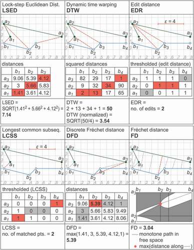
Each of the following subsections begins by presenting the basic definition of each similarity measure. Except for unifying notation, we have tried to keep the definitions as close as possible to the variants most widely adopted. (Figure 1) serves as a graphical summary of the computation of each measure.

Figure 1. Demonstration of trajectory similarity measures, aligning two trajectories where $\mathrm{n}$=3 and $\mathrm{m}$=4 (except for LSED, where $\mathrm{n}$=$\mathrm{m}$=3) according to the various measures, along with a corresponding distance matrix or free-space diagram. The distances relevant for computing the respective similarity measures are added as dashed red lines in the figures and highlighted in red in the matrices, e.g. distance $\mathrm{d}\mathrm{i}\mathrm{s}\mathrm{t}\left({\mathrm{a}}_3,{\mathrm{b}}_2\right)$ for DFD. Other relevant distances, included in the computation but not contributing to the final similarity measure, are also highlighted in gray cells, and gray dashed lines in associated geometric figures (in cases where associated distance is greater than zero). Further details of the precise computation of each measure are contained in Sections 4.1–4.6 below.

Lock-step Euclidean distance (LSED)

Lock-step Euclidean distance measures the total distance between all pairs of corresponding points in two trajectories. In the continuous setting, lock-step Euclidean distance requires that two trajectories are the same length. In the discrete setting, lock-step Euclidean distance requires two trajectories to contain the same number of points, or that we can interpolate along the length of the trajectories.

More formally, if $\mathrm{n}=\mathrm{m}$ we can interpret the trajectories as points in the Euclidean space ${\mathbb{R}}^{2\mathrm{n}}$ and take their Euclidean distance.

Definition 1. The lock-step Euclidean distance of $\mathrm{A}$ and $\mathrm{B}$ is defined as

(3) $\mathrm{E}\mathrm{u}\left(\mathrm{A},\mathrm{B}\right)=\sqrt{\sum _{\mathrm{i}=1}^{\mathrm{n}}{\mathrm{d}\mathrm{i}\mathrm{s}\mathrm{t}}_2^2\left({\mathrm{a}}_{\mathrm{i}},{\mathrm{b}}_{\mathrm{i}}\right)}.$(3)

A frequently used variant is the average distance between corresponding measurements:

(4) $\mathrm{E}{\mathrm{u}}^{\prime }\left(\mathrm{A},\mathrm{B}\right)=\frac{1}{\mathrm{n}}\sum _{\mathrm{i}=1}^{\mathrm{n}}\mathrm{d}\mathrm{i}\mathrm{s}{\mathrm{t}}_2\left({\mathrm{a}}_{\mathrm{i}},{\mathrm{b}}_{\mathrm{i}}\right).$(4)

Alternatively, the maximum instead of the average distance can be used. For example, in (Figure 1) the two trajectories have an average-distance LSED of 3.73 and a maximum-distance LSED of 5.66.

The definition above is most meaningful when there is a correspondence in time between the two trajectories. That is, if ${\mathrm{t}}_{\mathrm{i}}^{\mathrm{a}}={\mathrm{t}}_{\mathrm{i}}^{\mathrm{b}}$ for all $1\le \mathrm{i}\le \mathrm{n}=\mathrm{m}$, then LSED measures how far the trajectories are apart at corresponding times. In particular, $\mathrm{E}{\mathrm{u}}^{\prime }\left(\mathrm{A},\mathrm{B}\right)$ is then the average distance at corresponding times. If we assume uniform sampling in time, then the requirement n=m corresponds to both trajectories having the same duration, i.e. ${\mathrm{t}}_{\mathrm{n}}^{\mathrm{a}}-{\mathrm{t}}_1^{\mathrm{a}}={\mathrm{t}}_{\mathrm{n}}^{\mathrm{b}}-{\mathrm{t}}_1^{\mathrm{b}}$. However, if both trajectories have the same duration but use different – possibly non-uniform – sampling, then we can generalize these measures using interpolation:

(5) $\mathrm{E}\mathrm{u}\left(\mathrm{A},\mathrm{B}\right)=\frac{1}{\mathrm{n}}\underset{0}{\overset{{\mathrm{t}}_{\mathrm{n}}^{\mathrm{a}}-{\mathrm{t}}_1^{\mathrm{a}}}{\int }}\mathrm{d}\mathrm{i}\mathrm{s}{\mathrm{t}}_2\left(\mathrm{A}\left({\mathrm{t}}_1^{\mathrm{a}}+\mathrm{t}\right),\mathrm{B}\left({\mathrm{t}}_1^{\mathrm{b}}+\mathrm{t}\right)\right)\mathrm{d}\mathrm{t},$(5)

where $\mathrm{A}\left(\mathrm{t}\right)$ and $\mathrm{B}\left(\mathrm{t}\right)$ are the locations of $\mathrm{A}$ and $\mathrm{B}$, respectively, obtained by interpolation. Most commonly linear interpolation is used for this, i.e. for ${\mathrm{t}}_{\mathrm{i}}^{\mathrm{a}}\le \mathrm{t}\le {\mathrm{t}}_{\mathrm{i}+1}^{\mathrm{a}}$ we have:

(6) $\mathrm{A}\left(\mathrm{t}\right)={\mathrm{a}}_{\mathrm{i}}\frac{{\mathrm{t}}_{\mathrm{i}+1}^{\mathrm{a}}-\mathrm{t}}{{\mathrm{t}}_{\mathrm{i}+1}^{\mathrm{a}}-{\mathrm{t}}_{\mathrm{i}}^{\mathrm{a}}}+{\mathrm{a}}_{\mathrm{i}+1}\frac{\mathrm{t}-{\mathrm{t}}_{\mathrm{i}}^{\mathrm{a}}}{{\mathrm{t}}_{\mathrm{i}+1}^{\mathrm{a}}-{\mathrm{t}}_{\mathrm{i}}^{\mathrm{a}}}.$(6)

This interpolation assumes that the object moves between two measurements with constant speed along a straight line; an alternative is to bound these distances only assuming an upper bound on the speed of movement (Buchin and Purves 2013). All the distances above can be computed in $\mathrm{O}\left(\mathrm{n}+\mathrm{m}\right)$ time by scanning over the data once.

The Euclidean distance between two trajectories and its variants are widely used (cf. (Vlachos, Gunopulos, and Kollios 2002)). An implicit assumption underlying LSED is that the two trajectories are aligned in time. All of the following measures relax this condition: data points with different time stamps may be aligned as long as the alignment preserves the order of the points along the trajectories. For all of the measures the alignment is optimized according to certain criteria. The measures differ in the specific criteria.

Dynamic time warping (DTW)

Dynamic time warping is a classical dynamic-programming algorithm, originally used for speech recognition. DTW has been successfully applied to time series data since the work by (Berndt and Clifford 1994). Later, it became one of the most common methods for measuring similarity between trajectories. The following definition follows the one presented by (Chen, Özsu, and Oria 2005).

Definition 2. The dynamic time warping distance from A to B is defined as

(7) $\mathrm{D}\mathrm{T}\mathrm{W}\left(A,B\right)=\left\{\begin{array}{c}0\mathrm{i}\mathrm{f}\mathrm{A}\mathrm{a}\mathrm{n}\mathrm{d}\mathrm{B}\mathrm{a}\mathrm{r}\mathrm{e}\mathrm{e}\mathrm{m}\mathrm{p}\mathrm{t}\mathrm{y}\\ \mathrm{\infty }\mathrm{i}\mathrm{f}\mathrm{A}\mathrm{o}\mathrm{r}\mathrm{B}\mathrm{a}\mathrm{r}\mathrm{e}\mathrm{e}\mathrm{m}\mathrm{p}\mathrm{t}\mathrm{y}(\mathrm{n}\mathrm{o}\mathrm{t}\mathrm{b}\mathrm{o}\mathrm{t}\mathrm{h})\\ {\mathrm{d}\mathrm{i}\mathrm{s}\mathrm{t}}_2^2\left(a_1,b_1\right)+\mathrm{m}\mathrm{i}\mathrm{n}(\hspace{0.17em}\\ \mathrm{D}\mathrm{T}\mathrm{W}\left(A_{\left[2,n\right]},B_{\left[2,m\right]}\right),\hspace{0.17em}\\ \mathrm{D}\mathrm{T}\mathrm{W}\left(A,B_{\left[2,m\right]}\right),\hspace{0.17em}\\ \mathrm{D}\mathrm{T}\mathrm{W}\left(A_{\left[2,n\right]},B\right))\mathrm{o}\mathrm{t}\mathrm{h}\mathrm{e}\mathrm{r}\mathrm{w}\mathrm{i}\mathrm{s}\mathrm{e}\end{array}\right.$(7)

Matrix formulation

For this algorithm and several of the following ones, it will be insightful to interpret the distance definitions in terms of paths in the distance matrix between the trajectory points, illustrated in (Figure 1), for two sample trajectories $\mathrm{A}$ and $\mathrm{B}$. In the figure, the rows and columns of the matrix are laid out such that the squared distance between the first two points is at the lower left and the last two points at the upper right corner of the matrix.

Dynamic time warping can be seen as selecting a minimum cost path in the distance matrix. More precisely, DTW selects a path from the lower left to the upper right corner of the distance matrix that minimizes the sum of squared distances. In the example, the resulting sum is $2+13+34+1=50$. DTW is based on defining a cost for aligning two data points, namely the squared Euclidean distance between them.

From the point of view of walking along this path, from the lower left to the upper right corner, at each step DTW considers three possible moves: horizontal, vertical or diagonal. More specifically, the options available are:

1. Match current pair of points, and move diagonally: the cost of this move is equal to the squared distance between the pair of points.

2. Match current pair of points, and move up: the cost is equal to the squared distance between the pair of points.

3. Match current pair of points, and move right: the cost is equal to the squared distance between the pair of points.

Another useful way to visualize the DTW approach is in terms of alignments. Each path in the distance matrix considered by DTW corresponds to an alignment between the points of the two trajectories (red dashed lines, Figure 1). Each cell in the path implicitly aligns one point of $\mathrm{A}$ with one of $\mathrm{B}$, that is, a path through cell $\left(\mathrm{i},\mathrm{j}\right)$, for $1\le \mathrm{i}\le \mathrm{n}$ and $1\le \mathrm{j}\le \mathrm{m}$, is implicitly aligning ${\mathrm{a}}_{\mathrm{i}}$ with ${\mathrm{b}}_{\mathrm{j}}$.

What characterizes a similarity measure like DTW is how the cost of a path is defined, since the cost of a path represents how well the two trajectories are aligned in that path. Following (Chen, Özsu, and Oria 2005), in the definition above the cost of a path is the sum of the squared distances between all pairs of aligned points. In common with other measures using squared distance, this distance metric can help support tolerance to outliers, discussed further in Sections 5.6 and 8. However, DTW is also frequently used with other costs, e.g. turning angles, discussed in more detail at the end of this section. It is also common to enforce additional constraints on the path, for instance enforcing similar time-stamps between aligned measurements (see, e.g. (Keogh and Ratanamahatana 2005)).

Normalization

The DTW distance corresponds to a sum of squared distances between data points and depends on the number of data points used. This makes it difficult to compare DTW distances between different numbers of data points in each trajectory. In the experiments, we therefore divide the DTW distance by $\mathrm{m}\mathrm{a}\mathrm{x}\left(\mathrm{m},\mathrm{n}\right)$, which is (in the matrix formulation) the smallest number of cells that need to be visited. To obtain a more comprehensible 1D-distance measure, we additionally take the square root, that is, as normalized DTW distance we use $\sqrt{\mathrm{D}\mathrm{T}\mathrm{W}\left(\mathrm{A},\mathrm{B}\right)/\mathrm{m}\mathrm{a}\mathrm{x}\left(\mathrm{m},\mathrm{n}\right)}$, which produces $\sqrt{50/4}=3.54$ for the example in (Figure 1).

It might seem natural to normalize using the number of values in the sum (in terms of the matrix formulation: the number of cells visited) instead of $\mathrm{m}\mathrm{a}\mathrm{x}\left(\mathrm{m},\mathrm{n}\right)$. This approach would however make the normalized distance dependent on the path in the matrix, assigning relatively smaller normalized distances to longer paths.

Algorithm

The dynamic time warping distance is computed using dynamic programming, meaning that in terms of the formulation above one can compute for every cell(i,j) the cost of the best path to reach it. This computation requires constant time per cell, as a cell’s cost can be computed based on the cost of the cell left, below, and diagonally (left-below), resulting in an overall quadratic, i.e. $\mathrm{O}\left(\mathrm{n}\mathrm{m}\right)$, computation time. In practice, this can often be reduced to linear time, by carefully avoiding the computation for cells that have no influence on the final result (Keogh and Ratanamahatana 2005). To decrease the computation time further, deep neural network-based models have been developed for the DTW measure, see for instance (Zhang et al. 2019).

Edit distance (EDR)

Originally proposed to measure how similar two strings of characters are, edit distances have been successfully used for trajectory similarity. Conceptually, edit distance measures the changes (“edits”) to a trajectory – for instance, deleting a data point – needed to morph it into another trajectory. Every edit comes at a cost. Here we present the variant proposed by (Chen, Özsu, and Oria 2005), known as edit distance on real sequence (EDR). In this variant every edit has a unit cost, and the edit operations are either deleting a point, or aligning two dissimilar points.

Definition 3. The edit distance on real sequence (EDR) of $\mathrm{A}$ and $\mathrm{B}$ is defined as

(8) $EDR(A,B)=\{\begin{array}{l}nifBisempty\\ m;ifAisempty\\ \min (\\ EDR(A_{\left|2,n\right|},B_{\left|2,m\right|})+penalty(a_1,b_1),\\ EDR(A,B_{\left|2,m\right|})+1,\\ EDR(A_{\left|2,n\right|},B)+1)othervice\end{array}$(8)

where $\mathrm{p}\mathrm{e}\mathrm{n}\mathrm{a}\mathrm{l}\mathrm{t}\mathrm{y}\left({\mathrm{a}}_1,{\mathrm{b}}_1\right)$ is 0 if $\mathrm{d}\mathrm{i}\mathrm{s}{\mathrm{t}}_{\mathrm{\infty }}\left({\mathrm{a}}_1,{\mathrm{b}}_1\right)<\in$, or 1 otherwise.

The definition uses a parameter as a matching threshold distance (i.e. two points closer than $\in$ are considered to match).

Matrix formulation

Similar to DTW, EDR searches for a minimum cost path in the distance matrix, although it uses a matrix where the cost is defined differently. The cost of the path is the number of horizontal, vertical, and diagonal steps, excluding diagonal steps for which the corresponding pair of points are considered to match (i.e. their distance is smaller than).

It is important to note that in EDR costs are thresholded to 0 if the current pair of points match, whereas in all other situations the cost is 1, irrespective of the distance between the current pair of points. This results in the distance threshold matrix, a Boolean matrix as shown in (Figure 1). However, non-thresholded versions also exist. For instance, EDR itself is an adaptation of a measure proposed by (Cai and Ng 2004) called edit distance with real penalty (ERP). Instead of penalizing by 1 every time two elements do not match, ERP penalizes with the squared distance between the non-matching elements.

In terms of alignments, EDR defines the cost of a path as the number of aligned points that are not considered a match.

Algorithm

Computing edit distances can be implemented in the same way as DTW and therefore take quadratic time, $\mathrm{O}\left(\mathrm{n}\mathrm{m}\right)$, in the worst case.

Longest common subsequence (LCSS)

Longest common subsequence measures try to capture how well two trajectories match by measuring the length of the longest point sequence that they have in common. LCSS measures are closely related to edit distances, defined as follows after (Vlachos, Gunopulos, and Kollios 2002).

Definition 4. The length of the longest common subsequence between $\mathrm{A}$ and $\mathrm{B}$ is defined as

(9) $\mathrm{L}\mathrm{C}\mathrm{S}\mathrm{S}\left(A,B\right)=\left\{\begin{array}{c}0\mathrm{i}\mathrm{f}\mathrm{A}\mathrm{o}\mathrm{r}\mathrm{B}\mathrm{i}\mathrm{s}\mathrm{e}\mathrm{m}\mathrm{p}\mathrm{t}\mathrm{y}\\ 1+\mathrm{L}\mathrm{C}\mathrm{S}\mathrm{S}\left(A_{\left[1,n-1\right]},B_{\left[1,m-1\right]}\right)\mathrm{i}\mathrm{f}\mathrm{d}\mathrm{i}\mathrm{s}{\mathrm{t}}_{\mathrm{\infty }}\left(a_n,b_m\right)<\text{isin}\mathrm{a}\mathrm{n}\mathrm{d}\\ \hspace{0.17em}\left|n-m\right|\le \delta \\ \mathrm{m}\mathrm{a}\mathrm{x}(\mathrm{L}\mathrm{C}\mathrm{S}\mathrm{S}\left(A_{\left[1,n-1\right]},B\right),\hspace{0.17em}\\ \mathrm{L}\mathrm{C}\mathrm{S}\mathrm{S}\left(A,B_{\left[1,m-1\right]}\right))\mathrm{o}\mathrm{t}\mathrm{h}\mathrm{e}\mathrm{r}\mathrm{w}\mathrm{i}\mathrm{s}\mathrm{e}\end{array}\right.$(9)

The definition uses two parameters, $\delta$ and $\in$. As in EDR, $\in$ is a matching threshold distance (i.e. two points closer than $\in$ are considered to match). Additionally, $\delta$ controls how far in time (specifically, in timesteps) two matching points can be, in order to align the trajectories in time. However, it should be noted that $\delta$ is not specific to LCSS, and could be added to any of the other measures.

Matrix formulation

LCSS also looks for a path in its distance matrix (Figure 1), although with a few differences with respect to the previous measures. First, the path is searched in the opposite direction: from the upper right to the lower left corner. This is an arbitrary decision: it is easy to modify the formula to go in the same direction as DTW and EDR. But we preferred here to follow the original formulation from (Vlachos, Gunopulos, and Kollios 2002). The salient difference in LCSS is that the goal is to find a path of maximum score, with the objective to maximize the number of matched points. The score of a path is the number of diagonal steps, where diagonal steps are only allowed if points are similar.

In common with to EDR, LCSS is thresholded, meaning whether the point pairs match or not matters, but not the magnitude of difference. In terms of alignments, LCSS defines the value of a path as the number of alignments considered a match, making LCSS a measure that is somewhat complementary to EDR. Indeed, ignoring that one measure minimizes a cost and the other maximizes a score, the difference between LCSS and EDR is subtle: EDR allows diagonal steps for dissimilar points (at a cost), while LCSS does not.

Algorithm

As before, LCSS can be implemented using dynamic programming, and therefore takes quadratic time, $\mathrm{O}\left(\mathrm{n}\mathrm{m}\right)$, in the worst case.

Now we can define a similarity function based on LCSS.

Definition 5. LCSS-based similarity measure and distance definitions for two trajectories $\mathrm{A}$ and $\mathrm{B}$.

(10) $\mathrm{S}\left(\mathrm{A},\mathrm{B}\right)=\frac{\mathrm{L}\mathrm{C}\mathrm{S}\mathrm{S}\left(\mathrm{A},\mathrm{B}\right)}{\mathrm{m}\mathrm{i}\mathrm{n}\left(\mathrm{n},\mathrm{m}\right)}$(10)

(11) $\mathrm{D}\left(\mathrm{A},\mathrm{B}\right)=1-\mathrm{S}\left(\mathrm{A},\mathrm{B}\right)$(11)

(Vlachos, Gunopulos, and Kollios 2002) also give a second similarity measure that is invariant to translations, but here we only present the simplest version.

Discrete Fréchet distance (DFD)

Proposed by (Eiter and Mannila 1994), DFD can be seen as a version of DTW that takes the maximum distance between aligned points along the path. This is in contrast to DTW, which considers the sum of all squared distances.

Definition 6. The discrete Fréchet distance of $\mathrm{A}$ and $\mathrm{B}$ is defined as

(12) $\mathrm{D}\mathrm{F}\mathrm{D}\left(\mathrm{A},\mathrm{B}\right)=\left\{\begin{array}{cc}0& \mathrm{i}\mathrm{f}\mathrm{A}\mathrm{a}\mathrm{n}\mathrm{d}\mathrm{B}\mathrm{a}\mathrm{r}\mathrm{e}\mathrm{e}\mathrm{m}\mathrm{p}\mathrm{t}\mathrm{y}\\ \mathrm{\infty }& \mathrm{i}\mathrm{f}\mathrm{A}\mathrm{o}\mathrm{r}\mathrm{B}\mathrm{a}\mathrm{r}\mathrm{e}\mathrm{e}\mathrm{m}\mathrm{p}\mathrm{t}\mathrm{y}(\mathrm{n}\mathrm{o}\mathrm{t}\mathrm{b}\mathrm{o}\mathrm{t}\mathrm{h})\\ \mathrm{m}\mathrm{a}\mathrm{x}(\mathrm{d}\mathrm{i}\mathrm{s}{\mathrm{t}}_2\left({\mathrm{a}}_1,{\mathrm{b}}_1\right),\mathrm{m}\mathrm{i}\mathrm{n}(& \hspace{0.17em}\\ \mathrm{D}\mathrm{F}\mathrm{D}\left({\mathrm{A}}_{\left[2,\mathrm{n}\right]},{\mathrm{B}}_{\left[2,\mathrm{m}\right]}\right),& \hspace{0.17em}\\ \mathrm{D}\mathrm{F}\mathrm{D}\left(\mathrm{A},{\mathrm{B}}_{\left[2,\mathrm{m}\right]}\right),& \hspace{0.17em}\\ \mathrm{D}\mathrm{F}\mathrm{D}\left({\mathrm{A}}_{\left[2,\mathrm{n}\right]},\mathrm{B}\right))& \mathrm{o}\mathrm{t}\mathrm{h}\mathrm{e}\mathrm{r}\mathrm{w}\mathrm{i}\mathrm{s}\mathrm{e}\end{array}\right.$(12)

Matrix formulation

Similar to DTW and EDR, DFD searches for a minimum cost path in the distance matrix, from the lower left to the upper right corner (Figure 1). As in DTW, the cost of a pair is measured by taking the Euclidean distance.

In terms of alignments, DFD defines the cost of a path as the maximum over the distances between all pairs of aligned points. Note that taking the squared distance instead of the distance would result in the same optimal paths. Essentially, DFD’s difference to DTW is that it takes the maximum instead of the sum of the distances between all pairs of aligned points.

Algorithm

As before, DFD can be implemented using dynamic programming, resulting in an $\mathrm{O}\left(\mathrm{n}\mathrm{m}\right)$-time algorithm.

Fréchet distance (FD)

All the distance measures above are discrete, in the sense that they only align the measured locations ${\mathrm{a}}_{\mathrm{i}}$, ${\mathrm{b}}_{\mathrm{i}}$. This can potentially lead to problems for non-uniform sampling. In this section, we present the Fréchet distance (Alt and Godau 1995), which is also based on the maximum distance between the alignments, as DFD. However, in FD the alignments considered are continuous, meaning that they are taken between all points in both trajectories, by using the interpolated trajectories $\mathrm{A}\left(\mathrm{s}\right),\mathrm{B}\left(\mathrm{t}\right)$ (defined as in Formula 13).

Definition 7. The Fréchet distance between $\mathrm{A}$ and $\mathrm{B}$ is defined as

(13) $\mathrm{F}\left(\mathrm{A},\mathrm{B}\right)=\underset{\sigma }{\mathrm{i}\mathrm{n}\mathrm{f}}\underset{\mathrm{t}\in \left[{\mathrm{s}}_1,{\mathrm{s}}_{\mathrm{n}}\right]}{\mathrm{m}\mathrm{a}\mathrm{x}}\mathrm{d}\mathrm{i}\mathrm{s}{\mathrm{t}}_2\left(\mathrm{A}\left(\mathrm{t}\right),\mathrm{B}\left(\sigma \left(\mathrm{t}\right)\right)\right),$(13)

where the infimum is taken over all continuous, strictly monotone-increasing functions $\sigma :\left[{\mathrm{s}}_1,{\mathrm{s}}_{\mathrm{n}}\left]\to \right[{\mathrm{t}}_1,{\mathrm{t}}_{\mathrm{m}}\right]$ (i.e. all continuous alignments).

Algorithm

Algorithms to compute the Fréchet distance usually solve as a subroutine of the decision problem: to decide whether the Fréchet distance is smaller than a given $\in >0$. Given an algorithm for the decision problem, the Fréchet distance can be approximated by using a binary search over $\in$. A more complex search procedure, such as parametric search, can be used to compute the Fréchet distance exactly (Alt and Godau 1995).

The Fréchet decision problem can be solved by a dynamic programming algorithm. Consider the so-called free-space diagram in (Figure 1) (bottom right). The free-space diagram is the continuous analog to the distance threshold matrix used for the edit distance and LCSS. In the free-space diagram the vertical axis corresponds to the parameter space of $\mathrm{A}$ and the horizontal axis to the parameter space of $\mathrm{B}$. Thus, the point $\left(\mathrm{s},\mathrm{t}\right)$ in the diagram corresponds to the pair of points $\left(\mathrm{A}\left(\mathrm{s}\right),\mathrm{B}\left(\mathrm{t}\right)\right)$. The free space for a given $\in >0$ is the set of points $\left(\mathrm{s},\mathrm{t}\right)$ with the property that the distance between $\mathrm{A}\left(\mathrm{s}\right)$ and $\mathrm{B}\left(\mathrm{t}\right)$ is at most $\in$ .

In (Figure 1), the free-space diagram for $\in \approx 3.04$ is the white-colored region. The Fréchet distance is at most $\in$ if and only if there is a path from the lower-left corner to the upper-right corner that goes through the free-space and is monotonically increasing in both coordinates (shown in light gray). To compute whether such a path exists, we can incrementally compute the part of the free-space diagram that is reachable by such a path. This results in an $\mathrm{O}\left(\mathrm{m}\mathrm{n}\right)$-time algorithm for the decision problem. Computing the exact Fréchet distance then requires an additional $\mathrm{O}\left(\mathrm{l}\mathrm{o}\mathrm{g}\left(\mathrm{m}\mathrm{n}\right)\right)$ factor for the parametric search (Alt and Godau 1995). In the example of (Figure 1) the exact Fréchet distance is approximately 3.04 as the white region would disconnect when $\in$ is decreased any further. The corresponding alignment is shown as a dashed red line.

Discussion of conceptual and theoretical analysis

Following our pen-and-paper conceptual and theoretical analysis, and before moving on the experimental exploration, this section summarizes the key differences between the similarity measures.

Metric versus non-metric

LSED, DFD, and FD are metrics. DTW, LCSS, and EDR are not metics because:

• DTW does not obey the triangle inequality;

• LCSS does not measure difference (instead measuring, to some extent, similarity), although variants that satisfy some weaker conditions can be defined (Vlachos, Gunopulos, and Kollios 2002); and

• EDR does not fulfill two of the conditions of a metric, namely the identity of indiscernibles ($\mathrm{D}\left(\mathrm{A},\mathrm{B}\right)=0$ if and only if $\mathrm{A}=\mathrm{B}$) and the triangle inequality (D(A,B)+D(B,C)≥D(A,C)).

However, in general edit distance may be a metric, including some variants of edit distance used for time-series analysis, such as edit distance with real penalty (Cai and Ng 2004).

Discrete versus continuous

Fréchet distance (FD) is the only one of the similarity measures considered here that is continuous. FD works by finding a continuous alignment: one between the complete path of both trajectories, not just between trajectory fixes. Continuous measures are more natural when the interpolated values between trajectory points are relevant. Moreover, continuous measures are better suited to handling trajectories with differing sampling rates and gaps.

To illustrate, consider how the discrete versus continuous measures change in the presence of a data gap, leading to one long trajectory segment. Discrete measures will only consider the endpoints of that segment, producing an increase in the similarity measure. In the case of measures based on the sum of distances (e.g. LSED, DTW, EDR, LCSS), this increase may average out. However, measures that are based on the maximum distance (e.g. DFD) will drastically increase. In contrast, a continuous measure is likely to show the smallest effect in the presence of gaps or different sampling rates, as long as the points on the interior of long segments can be aligned to nearby points on the other trajectory.

Implementing a continuous measure does present additional computational challenges, as opposed to the relative simplicity of a discrete measure. However, the worst-case running time of the FD is only slightly worse than that of the other measures, $\mathrm{O}\left(\mathrm{m}\mathrm{n}\mathrm{l}\mathrm{o}\mathrm{g}\left(\mathrm{m}\mathrm{n}\right)\right)$ as opposed to $\mathrm{O}\left(\mathrm{m}\mathrm{n}\right)$, see Section 4.6 and (Alt and Godau 1995). Indeed, just as FD was described as a continuous version of the DFD, continuous versions of some other measures have also been defined. The so-called partial Fréchet distance (Buchin, Buchin, and Wang 2009) is the continuous analog of LCSS. For a given $\in >0$, the partial Fréchet distance aligns two trajectories to maximize the parts that have distance at most $\in$, measuring the overall length of these parts. The summed or average Fréchet distance is a continuous version of dynamic time warping, and aligns the trajectories as to minimize the average distance between matched points (Buchin 2007). Continuous versions of dynamic time warping using other measures for the pairwise distance between matched points have also been considered (Efrat, Fan, and Venkatasubramanian 2007).

Relative versus absolute time

LSED is the only similarity measure considered that expects measurements to be compared at corresponding times (possibly after an absolute time shift). Common to all of the other similarity measures discussed – DTW, ED, LCSS, DFD, and FD – is the principle of temporally aligning the two trajectories by aggregating the local costs (i.e. the cost of the temporal alignment between each pair of points). The key differences between measures often lie in the details of how this is done. For instance, DTW and DFD fundamentally differ only on whether to take the sum (DTW) or the maximum (DFD) of the local costs. This difference has knock-on impacts on how local time differences influence the measure. For instance, since DTW adds up the distance values of the cells visited (in the matrix formulation), it is of advantage to visit fewer cells, and therefore to take diagonal steps unless there is a bigger gain in terms of the local cost by taking horizontal/vertical steps. For all the measures, how much local variation in time is allowed can be restricted by restricting the path in the distance matrix to cells close to the diagonal (or more generally, close to the path that corresponds to a perfect alignment in time). The extreme case where the path is completely restricted corresponds to LSED (or a variant thereof).

As discussed in Section 3.3.2, all similarity measures encountered are sensitive to the order of points in trajectories. The in-built temporal alignment of trajectory measures, discussed above, will not aid in identifying similar but “inverse” trajectories, where the same spatial path is followed in the opposite direction (e.g. comparing home to work and work to home trajectories). However, it is possible to conceive of temporal transformations that would help in identifying such trajectory similarities.

For example, when comparing two trajectories $\mathrm{A}$ and ${\mathrm{A}}^{\prime }$, where ${\mathrm{A}}^{\prime }$ traces the same spatial path as $\mathrm{A}$ but in the opposite direction, it is possible to compare instead two temporally transformed trajectories $\mathrm{B}$ and ${\mathrm{B}}^{\prime }$, such that:

$\mathrm{B}=\left(\left({\mathrm{p}}_{\mathrm{i}}^{\mathrm{a}},{\mathrm{t}}_{\mathrm{i}}^{\mathrm{a}}-{\mathrm{t}}_1^{\mathrm{a}}\right),\dots ,\left({\mathrm{p}}_{\mathrm{n}}^{\mathrm{a}},{\mathrm{t}}_{\mathrm{n}}^{\mathrm{a}}-{\mathrm{t}}_1^{\mathrm{a}}\right)\right)\mathrm{a}\mathrm{n}\mathrm{d}{\mathrm{B}}^{\prime }=\left(\left({\mathrm{p}}_{\mathrm{j}}^{{\mathrm{a}}^{\prime }},{\mathrm{t}}_{\mathrm{m}}^{{\mathrm{a}}^{\prime }}-{\mathrm{t}}_{\mathrm{j}}^{{\mathrm{a}}^{\prime }}\right),\dots ,\left({\mathrm{p}}_{\mathrm{m}}^{{\mathrm{a}}^{\prime }},{\mathrm{t}}_{\mathrm{m}}^{{\mathrm{a}}^{\prime }}-{\mathrm{t}}_{\mathrm{m}}^{{\mathrm{a}}^{\prime }}\right)\right)$

where ${\mathrm{t}}_{\mathrm{k}}^{\mathrm{x}}$ denotes the $\mathrm{k}$th timestamp in trajectory $\mathrm{X}$, as introduced in Section 4. In this case, computing the similarity of $\mathrm{B}$ and ${\mathrm{B}}^{\prime }$ will provide high levels of similarity corresponding to spatially coincident trajectories traversed in opposite directions $\mathrm{A}$ and ${\mathrm{A}}^{\prime }$.

Relative versus absolute space

The distance measures considered above align trajectories in time to minimize absolute Euclidean distances. However, depending on the application, relative distance may be more important. This is addressed in two different ways. The first approach is to take one of the measures above and optimize it under a suitable set of transformations, e.g. translations. That is, if $\mathrm{D}\left(\mathrm{A},\mathrm{B}\right)$ is a distance measure between trajectories $\mathrm{A}$ and $\mathrm{B}$, one would consider $\mathrm{m}\mathrm{i}\mathrm{n}(\{\mathrm{d}\left(\mathrm{A},\mathrm{B}+\tau \right)|\tau \in \mathrm{T}\})$, where $\mathrm{T}$ is the set of two-dimensional translations. This minimization problem is typically computationally expensive (see for example (Vlachos, Gunopulos, and Kollios 2002)), and often solved by sampling the space of transformations (Alt and Scharf 2012). The second approach is much simpler. Instead of using Euclidean distances, an alternative measure that is invariant under a suitable set of transformations is used. Common choices for this alternative include heading (translation-invariant) and turning angle (translation- and rotation-invariant). For instance, one can use DTW with turning angles instead of squared Euclidean distances. Note that the use of measures such as heading or turning angle complicates the application of continuous similarity measures such as FD, since it would require to interpolate heading or turning angle between trajectory points.

Computational efficiency

Regarding efficiency, the simplest and fastest measure discussed is LSED, as it only requires processing the input trajectories once, which takes $\mathrm{O}\left(\mathrm{n}+\mathrm{m}\right)$ time. Fréchet distance is least efficient $\mathrm{O}\left(\mathrm{n}\mathrm{m}\mathrm{l}\mathrm{o}\mathrm{g}\left(\mathrm{n}\mathrm{m}\right)\right)$, but also the subject of considerable recent efforts to improve efficiency (Bringmann, Künnemann, and Nusser 2019). The dynamic programming-based measures (DTW, EDR, LCSS and DFD) require $\mathrm{O}\left(\mathrm{n}\mathrm{m}\right)$ time in their standard formulations. The dynamic programming approach is also easy to implement, and is almost identical for all four measures. Theoretical improvements for some of these measures are possible (Agrawal and Dittrich 2002; Buchin et al. 2014; Masek and Paterson 1980). However, these are marginal improvements in practice and come at the cost of increased complexity of implementation. Approximating a similarity measure can also yield faster computation. For instance, limiting how much local time-shifting is allowed restricts the search to a smaller portion of the distance matrix (or free space diagram for the Fréchet distance) close to the diagonal.

Tolerance to outliers

One final important difference between the various measures is worth highlighting: tolerance to outliers. Generally, measures that use the maximum distance between matched points (such as FD and DFD) emphasize large distances and are therefore more sensitive to outliers than measures that use the sum of distances (or even the sum of squared distances). Thresholds (as used in the EDR and LCSS) can be useful for dealing with outliers as they allow for the assignment of a uniform cost to pairs that are matched but have a distance larger than the threshold. In this sense, LCSS can be interpreted as the measure that minimizes the number of points that need to be classified as outliers to perfectly align the remaining trajectories. This, however, comes at the cost of introducing the threshold as an additional parameter.

Experimental setup

The discussion in Section 4 provided a thorough theoretical analysis of the different trajectory similarity measures. Section 5 then provided summary of expectations of the behavior of different measures with respect to key characteristics, such as temporal alignment, tolerance to outliers, and computational efficiency. In Sections 6 and 7, we turn to exploring similarity through experiments with real data, to aid in discerning apart differences which may be theoretically important, but practically less relevant.

To throw light on the widest range of practical scenarios, we selected two benchmark trajectory data sets with sharply contrasting properties: vehicle movements through a transportation network, and trajectories capturing the behavior of coastal wading birds.

Data sets

The Dublin bus GPS sample data set (Dublin City Council 2013) was selected as our first data set. The data set records timestamped GPS coordinates of buses traveling around Dublin at a frequency of 20 seconds using on-board GPS devices. Each GPS fix is associated with a unique bus ID, journey ID, bus route ID, as well as route direction.

This data set was chosen as it is especially suitable for separating spatial and temporal aspects. For example, bus trajectories from the same time but different routes are expected to be relatively dissimilar. Trajectories from the same route but at different times are expected to be relatively similar. Such trajectories are subject to timing differences due to traffic and schedules, but are inherently spatially similar and will be automatically temporally aligned to some degree by all our similarity measures, excepting LSED (cf. Section 5.4). Trajectories from the same route at the same time on different week days are expected to be most similar.

To prepare a suitable set of bus trajectories for our experiments:

• From among tens of thousands of Dublin bus trajectories, a selected subset of 137 trajectories was extracted from weekdays (2nd, 3rd, 4th, and 7th of January 2013) and 8–9am, 1–2pm, and 8–9pm time blocks.

• Any stationary trajectory segments at the start or the end of a trajectory were removed, to avoid distorting similarity values with extended stops.

This subset of trajectories from restricted dates and times ensured sufficient pairs of trajectories at comparable locations and times for our experiments to test the responses of different similarity measures to different trajectory pairings. Two example pairs of trajectories are shown in (Figure 2).

Figure 2. Example bus trajectories. Dashes perpendicular to movement paths denote trajectory “fixes” (timestamped points in the trajectory). The left pair shows trajectories of the same bus route collected at the same time but on different days. The left pair are spatially coincident (same bus route), but have been displaced for visual clarity. This displacement was not employed during similarity calculation. The right pair shows trajectories with different routes and different times.

The second data set concerned GPS trajectories of oystercatchers, annotated with bird activities (Shamoun-Baranes et al. 2012). Specifically, this data set resulted from a one month-long 2009 scientific study of three oystercatchers, in a 3 km${ }^2$ region of Schiermonnikoog island in northern Netherlands. The trajectories used were derived from GPS trackers fitted to the birds generating fixes every 10s. During tracking, birds were simultaneously observed by the scientists through telescopes. These observations enabled the trajectories to be annotated with eight different types of behaviors: aggression, body care, fly, forage, handle, sit, stand, and walk.

This data set was chosen as it is especially suitable for exploring similarity of trajectories transformed in time and space. Bird trajectories reflecting the same activity may occur in different locations and times. The distinctive features of the different observed movement behaviors are expected to make the trajectories resulting from those behaviors dissimilar. An example of a “flight” and a “forage” trajectory are contrasted in (Figure 3).

Figure 3. Example bird trajectories, showing one trajectory of flight (black) and one trajectory of foraging (gray).

To prepare a suitable set of bird trajectories for our experiments:

• Those trajectories annotated as either flight or foraging were extracted from the full data set, to support comparisons between trajectories arising from known, different types of activities (and hence expected to exhibit different levels of similarity).

• Trajectories with a length of fewer than four fixes were excluded, judged to be too short to clearly indicate any embedded activity.

After the preprocessing and filtering step, there remained 870 trajectory segments. Due to the relative under-representation of flight behaviors in the underlying data set, only nine of these trajectories corresponded to flight behaviors. Nevertheless, this number was still deemed large enough set to run our experimental cross comparisons.

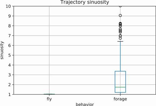
Visual inspection of the trajectories associated with different behaviors indicated apparent spatial differences, as expected. For example, oystercatchers appear to make more sudden turns when they are foraging compared to cases when they are simply flying (Figure 3). To confirm this visual impression, (Figure 4) shows the sinuosity of the two sets of trajectories extracted. Trajectories of flight behavior have uniformly a sinuosity close to 1 (a straight line). In contrast, forage behavior exhibits a wide variety of trajectories sinuosity, with an average sinuosity approaching 2.

Figure 4. Sinuosity comparison between fly trajectories and forage trajectories.

Measure thresholds and normalization

As the trajectories used in the experiments can vary dramatically in length, a direct comparison of similarity measures is not possible. In order for all similarity measures to be compared within the same categories, and between inter-category groups, LCSS and EDR similarity values needed to first be normalized. LCSS was normalized by the shortest trajectory length while EDR was normalized by the longest trajectory length. DTW was normalized as a function of the number of points in the longest trajectory in a pair (Section 4.2). As DFD and FD are essentially unaffected by length of trajectories, normalization was unnecessary.

The threshold value $\in$ for LCSS and EDR was set to 50 m for all experiments, except where stated.

Experimental results

This section presents the results of four experiments, structured so as to explore the behavior of the different trajectory similarity measures with increasingly dissimilar sets of paired trajectories drawn from the data sources introduced in the previous section. These experiments are designed to provide a baseline comparison (Experiment 1); explore trajectory similarity of movement in a constrained network space (Experiment 2); compare similarity measures in the context of different movement behaviors (Experiment 3); and contrast similarities of fundamentally different types of movement (Experiment 4).

Throughout these experiments it is important to emphasize that our focus remains on what the data and experiments can tell us about the differences between similarity measures, rather than what the similarity measures can tell us about the differences between the data sets. It is important not to lose sight of the fact our comparative analysis is primarily concerned with elucidating the characteristics similarity measures themselves, not the differences in trajectory data sets nor on the different movement behaviors that give rise to those trajectories.

Experiment 1: verification and baseline

Our first experiment explored the baseline differences between similarity measures under a range of transformations. Our expectation is that different similarity measures exhibit different levels of sensitivity to spatial, temporal, or spatiotemporal transformations.

A randomly selected trajectory was resampled to a single high-resolution baseline trajectory from the raw data (Figure 5(a)). The bus data set was used as the source of this baseline trajectory. However, this choice was arbitrary, and has no impact on the expected results in Experiment 1, which compare the effect of different transformations on measured similarity. Three further transformed trajectories for comparison were derived from this baseline as follows:

1. A temporal transformation, where points were sub-sampled from the original trajectory with an increasing temporal interval, clustering points toward the (temporal) beginning of the trajectory (Figure 5(b));

2. A spatial transformation where the base trajectory was rotated slightly about its origin (Figure 5(c)); and

3. A spatiotemporal transformation where both temporal and spatial transformations above were applied (Figure 5(d)).

Figure 5. Experiment 1 setup. Trajectory comparisons between one bus trajectory and its variations. The black trajectory is the baseline, with transformed gray trajectories showing (a) no transformation, (b) temporal transformation, i.e. measurements are temporally shifted toward one the beginning of the trajectory, (c) spatial transformation, i.e. the gray trajectory has been rotated, and (d) spatiotemporal transformation, i.e. the combination of both the spatial and the temporal transformation. In our figures, the gray trajectories have been additionally displaced for visual clarity, with (a) illustrating this purely visual transformation.

The threshold value $\in$ for LCSS and EDR was set to 100 m in Experiment 1, unlike subsequent experiments, where the threshold used was 50 m. The higher threshold was selected as the Experiment 1 baseline was the only case where the trajectories were resampled (see above).

Results

(Table 1) shows the calculated similarity measures for the trajectories shown in (Figure 5). The table shows both the absolute similarity measure computed, and in parenthesis the relative rank of that similarity across all four values computed for that measure.

Table 1. Computed similarities between black and gray trajectories in (Figure 5). The ranks in parentheses indicate for every measure the relative order of the computed similarities.

Transformation	None	Temporal	Spatial	Spatiotemporal
	(Figure 5(a))	(Figure 5(b))	(Figure 5(c))	(Figure 5(d))
LCSS Ratio	$1\left(1\right)$	$0.68\left(2\right)$	$0.61\left(3\right)$	$0.55\left(4\right)$
EDR Ratio	$0\left(1\right)$	$0.57\left(3\right)$	$0.43\left(2\right)$	$0.70\left(4\right)$
Fréchet (m)	$0\left(1\right)$	$163.61\left(2\right)$	$497.84\left(3=\right)$	$497.84\left(3=\right)$
Discrete Fréchet (m)	$0\left(1\right)$	$456.87\left(2\right)$	$497.84\left(3=\right)$	$497.84\left(3=\right)$
DTW (m)	$0\left(1\right)$	$179.64\left(2\right)$	$270.19\left(4\right)$	$259.10\left(3\right)$

Interpretation

We expected that all measures would yield maximum similarity when trajectories are identical. This expectation is indeed confirmed in (Table 1). Such a comparison can be seen as a trivial verification of the implementation of our code, and an important sanity check.

In all cases except LCSS, identical trajectories (i.e. no transformation, Figure 5) yield a value of 0. In other words, these measures strictly measure dissimilarity, with larger values indicating greater dissimilarity. LCSS in contrast does measure similarity, yielding a value of 1 for two identical trajectories.

Beyond these extreme values, though, in most cases a physical interpretation of the meaning of the similarity measures is not straightforward. EDR and LCSS were both normalized between 0 and 1 (see Section 6.2). DTW was normalized as a function of the number of points in the longest trajectory in a pair (Section 4.2). FD and DFD can be interpreted as a discrete physical distance. However, in general the magnitude of similarity values are hard to ascribe meanings to, and as a consequence absolute similarity values are hard to compare, except in the case of FD and DFD.

Instead, in this experiment, we are more interested in the ordering of results within and between similarity measures. Are the same trajectory pairs always more similar, irrespective of the similarity measure used? Or, as we expect from our theoretical analysis, are some measures more sensitive to spatial or temporal transformations than others?

Looking at (Table 1), it can be inferred that similarity values are indeed sensitive to the measures used, with both the absolute value and relative ranking of trajectory similarity varying between measures with different transformations used.

One further unanticipated difference is worth highlighting. The similarity values associated with continuous and discrete Fréchet distance under temporal transformations are notably different, where all other similarity values for FD and DFD are in accord. This difference arises since under FD distances are calculated between not only data points but also interpolated segments between these points, and thus the influence of the temporal transformation of the data points is limited.

Experiment 2: bus routes

Our second experiment aimed to explore the behavior of different similarity measures on real trajectories constrained in a network space. Here, we assumed that spatial behavior, while not identical, is very similar for repeated instances of the same route. Temporal behavior, however, may vary greatly (i.e. from variations in traffic flow) based on the time of day. A key question then is as follows: where similarity measures are better suited to discriminating between trajectories paired from different categories?

We chose two dimensions along which to characterize trajectories: spatial similarity, where we select trajectories according to individual bus routes; and temporal similarity, where we select trajectories from the three sampled time periods (8–9am, 1–2pm, and 8–9pm, all on weekdays). These criteria were then used to randomly select pairs of trajectories to test four scenarios:

• SameSame: 36 pairs of different trajectories, where both trajectories in each pair are derived from a bus traveling along same route in the same temporal window, possibly on different weekdays.

• SameRoute: 36 pairs of different trajectories, where both trajectories in each pair are derived from a bus traveling along the same route in different temporal windows.

• SameTime: 36 pairs of different trajectories, where both trajectories in each pair are derived from a bus traveling along different routes in the same temporal windows, possibly on different weekdays.

• DiffDiff: 36 pairs of different trajectories, where both trajectories in each pair are derived from a bus traveling along different routes in different temporal windows.

These four scenarios capture the essential spatial and temporal dimensions of trajectory similarity of tracking data in network space.

Results

(Figure 6) shows box plots of the similarity measures for each of our four cases. Hence, each box plot summarizes 144 data points.

Figure 6. Box plots of bus trajectory similarity. The five similarity measures are tested against four different scenarios, where the pair of trajectories of interest are of (1) same time same route; (2) same time different routes; (3) different time same route and (4) different time different routes.

It is immediately evident from (Figure 6) that the spatial differences between trajectories dominates the similarity values. For all similarity measures, SameSame and SameRoute, which compare the same spatial trajectory paths, exhibit higher levels of measured similarity than SameTime and DiffDiff, which compare different routes. By contrast, temporal differences appear to have little influence on measured similarity.

This observation was confirmed using a Wilcoxon signed rank hypothesis test. The test revealed no significant differences at the 5% level between either the SameSame versus SameRoute or the SameTime versus DiffDiff across all measures tested. By contrast, the differences between SameSame versus SameTime/DiffDiff and between the SameRoute versus SameTime/DiffDiff are significant at the 5% level in all cases.

Interpretation

In our second experiment, our expectation was that different similarity measures should be able to discriminate between trajectories that differ spatially, temporally, or spatiotemporally.

In fact, the results imply that differences between bus trajectories are largely the product of spatial differences. None of the treatments where differences were purely temporal (SameSame versus SameRoute or the SameTime versus DiffDiff) yielded statistically significant differences in similarity measure. Conversely, all of the treatments that varied the spatial path, whether independent of or in combination with temporal differences, resulted in significant differences in measured similarity.

Having said that it should be noted that bus routes are oftentimes designed to be spatially different in order to cover more area and share less overlap may be a factor in the lack of similarity between different routes, when compared with different times. Further, bus trajectories collected at different time periods are not necessarily temporally distinct in the way illustrated by the temporal transformation of a trajectory in Experiment 1. Instead, there appeared to be limited difference in the proportion of points at each section of the trajectory. This is likely due to buses following fixed schedules, operating at similar speeds, and stopping with similar frequency.

Experiment 3: bird behaviors

In Experiment 3 our aim was to assess trajectory similarity with respect to known behavioral differences between bird flight and foraging. In this experiment, pairs of trajectories were selected randomly from bird movements labeled as foraging or flight behavior, to build the following treatment sets:

• FlyFly: 36 pairs of different trajectories, constructed from exhaustive pairings of different trajectories from the set of 9 trajectories labeled as flight.

• FlyForage: 36 pairs of different trajectories, randomly selected one from the set labeled as flight and one from the set labeled as foraging.

• ForageForage: 36 pairs of different trajectories, randomly selected from the set of trajectories labeled as foraging.

The relatively small number of nine trajectories labeled as flight in our data set provided a lower bound for the number of pairs in our experiments ($(9-1{)}^2/2=36$). Although larger data sets might have been sought to increase this lower bound sample size, a well-known effect of increasing sample sizes is unwarranted inflation of the statistical significance of hypothesis tests, a particular hazard in the information sciences, where data sets may often be arbitrarily large (Lin, Lucas, and Shmueli 2013). Hence, our lower bound of 36 samples in each treatment set was deemed an appropriate sample size for our experimental cross comparisons, applied across all Experiments 2–4 using real data.

Since such bird movements were spatially dispersed, a necessary additional step in Experiment 3 was a geometric transformation (translation and rotation) to spatially align trajectories. Thus, all trajectories were translated such that their origins were identical, and rotated so that the angle formed between the first and last point in every trajectory was 45 degrees.

Results

Box plots showing the results for all five similarity measures across the three different treatment sets are shown in (Figure 7).

Figure 7. Box plots of bird activity trajectory similarity. The five similarity measures are tested against three scenarios, where the pairs of trajectories are (1) both from flight activity group; (2) one from flight and one from forage activity group; and (3) both from forage activity group.

In contrast to the previous experiment, the results indicate a clear difference between the five similarity measures. While pairs of foraging trajectories were ranked with higher similarity by Fréchet distance, DFD, and DTW, this was not the case for pairs of flight trajectories. Pairs of flight trajectories were measured using Fréchet distance, DFD, and DTW as at least as dissimilar as pairs of flying/foraging trajectories.

To test whether similarity measures could be treated as being drawn from different populations, according to the semantics of the comparisons, we performed a Kruskal-Wallis rank sum test (Table 2). As suggested by the box plots, we found significant differences (p$<$0.05) between the similarity values for Fréchet distance, DFD, and DTW only.

Table 2. P-values for Kruskal-Wallis test performed on the similarity distribution for analysis on Oystercatcher data.

	P-value	Significant at 5% level
LCSS Ratio	$0.3389$
EDR Ratio	$0.5583$
Fréchet	$0.0057$	*
Discrete Fréchet	$0.0057$	*
DTW	$0.0075$	*

To further explore the nature of these differences, we then performed pairwise Wilcoxon signed rank tests to compare the (FlyFly with FlyForage/ForageForage with FlyForage) (Table 3). We found significant differences (p$<$0.05) for both measures when comparing foraging behavior with mixed groups of trajectories, but were not able to distinguish between flying behavior from mixed groups. These results, given our previous experiment, imply that the form of trajectories has an influence on the sensitivity of measures to differences.

Table 3. P-values for Wilcoxon signed rank tests for analysis on Oystercatcher data.

	Comparison groups	P-value	Significant at 5% level
FD,DFD	FlyVsFly and FlyVsForage	0.4375
	ForageVsForage and FlyVsForage	0.0210	*
DTW	FlyVsFly and FlyVsForage	0.5625
	ForageVsForage and FlyVsForage	0.0210	*

Interpretation

It was expected that the different similarity measures would capture differences between behavioral patterns expressed through differing movements. More specifically, trajectories arising from the same activity were expected to be more similar than those arising from different activities.

In contrast, the results for EDR indicate this measure is unable to distinguish any of the exhibited movement patterns, with no significant differences found between treatment sets and all combinations of patterns approximately equally dissimilar.

The results for Fréchet distance, DFD, and DTW did indicate that foraging trajectories do share common features that are invariant to transformation, as expected. However, in the case of flight behavior, these three measures yielded similarity values indicating one flight trajectory may be as dissimilar from another flight trajectory as it is from a foraging trajectory.

The LCSS ratio is the only measure that appear to exhibit the expected signal – that pairs of flying and pairs of foraging trajectories have greater similarity than mixed pairs – albeit a signal that is weak and not significant at the 5% level.

Overall, the measures provided much weaker alignment with expectations in differentiating between labeled animal movement trajectories. It is worth noting that such comparisons are a typical example of trajectory similarity comparisons in a between-subjects experiment in ecology, where the aim is to describe animal behaviors using GPS tracks.

Experiment 4: buses vs birds

In any experiments comparing methods, it is important to consider straightforward baselines that are easy to interpret. Since the two data sets used exhibit very different properties, one final experiment was designed to compare these two more general activities – bird activity and bus activity.

The similarity measures were then performed on three treatment sets of trajectory pairs:

• BirdBird: 36 randomly selected pairs of different bird trajectories.

• BusBird: 36 randomly selected pairs of trajectories, one from the set of bird and one from the set of bus trajectories.

• BusBus: 36 randomly selected pairs of different bus trajectories.

As the bird and bus trajectories lie far away from each other, transformation in space and time was utilized to enable comparison. Trajectory pairs were translated and rotated in space and scaled in time to align the start and end points of both trajectories together.

Results

(Figure 8) shows box plots for trajectories selected from pairs of similar (BusBus and BirdBird) and dissimilar (BusBird) trajectories.

Figure 8. Box plots of bird and bus activity trajectory similarity. The five similarity measures are calculated for three scenarios: (1) Bird trajectory vs Bird trajectory; (2) Bus trajectory v.s. Bus trajectory and (3) Bus trajectory v.s. Bird trajectory.

From (Figure 8), Fréchet distance, DFD, and DTW all appear to be able to discriminate between semantically similar and dissimilar objects, with largest values (and thus most dissimilar) trajectories associated with the BusBird pairs. However, LCSS and EDR, while finding the greatest similarity between BirdBird pairs, found either higher dissimilarity (LCSS) or comparably high dissimilarity (EDR) between BusBus and BusBird pairs.

As for Experiment 3, pairwise Wilcoxon signed rank tests were performed in order to determine if there was a significant difference between the three groups of trajectory pairs. With the exception of the EDR ratio on BusBird and BusBus trajectory pairs, all other comparisons deferred exhibit significant differences at the 5% level.

Interpretation

Our final experiment compared trajectories from across our two data sets, to explore whether the similarity measures detect differences between fundamentally different types of behavior. Hence, this experiment provides a baseline for all experiments by comparing trajectories from markedly different domains that are expected to be intrinsically markedly different: buses moving in a structured network space versus birds free to move in a largely unconstrained space.

Our expectation was that bird and bus trajectories should be distinguishable based solely on their movement patterns. While the results broadly aligned with this expectation, neither LCSS nor EDR ratio were able to consistently reflect this expectation.

Conclusions and recommendations

This section draws together our conclusions from across all the three perspectives on trajectory similarity – conceptual, theoretical, and empirical – leading to high-level advice and recommendations for choosing trajectory similarity measures.

Summary of experimental perspective

Taking the observed differences across our four experiments, it is possible to identify three general empirical properties of the different similarity measures.

1. Differences in similarity values are sensitive to the choice of measure. In particular, not only does the absolute similarity value computed vary; but the relative ordering of similarity of trajectory pairs may vary across different similarity measures (e.g. Table 1).

2. All the similarity measures tested were more effective at distinguishing spatially dissimilar trajectories, when compared with temporally dissimilar trajectories. Relatively small spatial differences in trajectories tend to correspond to large differences in the magnitude of measured similarity, more so than even relatively large temporal differences in trajectories (e.g. Experiment 2, Section 7.2).

3. Broadly speaking, similarity values computed using DTW, DFD, and FD tended to accord more closely with our expectations of similarity than LCSS and EDR. In Experiment 3 (Section 7.3), for example, LCSS and EDR both failed to distinguish trajectories that arose from quite different activities, and were at least visually quite distinct (Figure 3). Similarly, in Experiment 4 (Section 7.4), the similarity values for EDR even failed to reliably discern apart differences between bus trajectory pair when compared with differences between bus and bird trajectories.

Summary of all perspectives

Metric measures

Some applications, such as indexing or clustering, rely on similarity measures that offer metric properties. In such cases only some of these similarity measures are suitable (LSED, DFD, FD, and possibly edit distance, although not EDR).

Discrete vs continuous measures

Only Fréchet distance, and its interpolation between measured locations, can provide a measure of difference over continuous trajectory paths, although some continuous analogs of DTW and LCSS can also offer continuous measure properties. The decision as to whether to use a discrete or a continuous measure usually depends on several aspects, such as whether the sampling rates in the trajectories are expected to be similar (e.g. in terms of density or frequency of fixes); whether interpolation between trajectory points is possible and meaningful; and the fact that discrete measures are typically simpler to implement.

Computational efficiency

A major factor to consider when selecting a similarity measure is computational efficiency. In terms of computational complexity (the rate at which computation time increases as a function of input data size), FD is the least efficient measure; LSED the most efficient; with DTW, LCSS, EDR, DFD falling in between these extremes, all underpinned by similar dynamic programming implementations. However, in practice throughout all of the experiments, little to no difference was found when comparing FD to its discrete counterpart. In all cases, the primary influence in execution time is the number of sample points in the trajectories, meaning that over-sampling should be avoided.

Maximum vs sum of distances

Similarity measures at root measure either the maximum of distance between trajectories (i.e. FD, DFD), or the sum of all or a sample of distances between trajectories (LSED, DTW, EDR, LCSS). Different measures in this respect may lend themselves to different applications. As a direct consequence, those measures that are based on maximum distances are much more sensitive to outliers than those based on the sum of distances. That said, in our experiments FD, DFD, and DTW performed similarly, indicating that any outliers present in our data sets were not sufficiently significant to influence the results.

Spatial vs temporal similarity

In all of the similarity measures tested, the spatial differences between trajectories were more important in determining the magnitude of measured similarity than temporal differences. This is particularly evident in Experiment 2. However, the precise magnitude of these differences is likely to depend strongly on the specific application.

Thresholds

This exploration has not covered the selection of meaningful thresholds for similarity measures that require them, EDR and LCSS. Neither theory nor the experiments in this paper can offer insights into the right thresholds to choose. Thresholds are highly data dependent, and their selection needs to take into account the specific characteristics of the application, including noise, outliers, and constrained or unconstrained spaces for movement.

Bounded versus unbounded measures

As noted among the five similarity measures, LCSS and ED can be expressed as ratios, bounded between $0$ and $1$. Fréchet distance, DFD, and DTW are unbounded positive numbers. Although bounded measures do enable similarity results to be compared across different data sets, they have low resolution when representing high dissimilarity. For example, while it is easy to define 0 in edit distance ratio as two trajectories that are identical, there is no situation where two trajectories are so different that they produce a value of $1$. Additionally, the lower discriminatory power poses significant issues when different types of trajectories are compared as evidenced by LCSS and EDR ratio’s inability to distinguish different movement patterns in Experiment 3.

Interpretation of measure magnitudes

Similarity measures are best interpreted in terms of relative ordering, rather than absolute magnitude. FD and DFD similarity measures do have a direct physical interpretation, as the maximum sum of differences between trajectories. Hence, similarity values computed using these measures may arguably be compared or reasoned about (e.g. two trajectories with an FD of 1000 m are arguably twice as dissimilar as a trajectory pair with an FD of 500 m). DTW similarly has a physical interpretation, albeit a less intuitive one (cf. Section 4.2). LCSS and EDR ratios have no such interpretation. However, given the limitations of similarity measures discussed above, such as their discriminatory power, and the experimental variability, it seems safer in all cases to interpret measured values qualitatively (i.e. more or less similar) rather than quantitatively.

Summary of recommendations

To conclude, (Table 4) provides a visual summary of the most salient differences between the similarity measures. The table indicates for each similarity measure whether it:

1. is a metric (is symmetric; obeys triangle inequality; and zero only when two compared objects are equal, see Section 3.1);

2. operates on discrete or continuous trajectories;

3. accommodates relative time by automatically aligning trajectories temporally;

4. is computationally efficient, when compared with other measures (in (Table 4) three stars indicates most efficient, one star least efficient);

5. is robust to outliers, when compared to other measures (in Table 4 three stars indicate most tolerant, one star least tolerant).

Table 4. Summary of differences in similarity measures, with reference to characteristics in Section 5. The star rating provides a summary of the relative computational efficiency and resilience to outliers (see Sections 5.5 and 5.6), with three stars being most efficient/tolerant and one star least efficient/tolerant. The color coding of cells similarly provides a visual impression of subjective “performance,” where lighter cells correspond to more desirable characteristics.

	LSED	DTW	EDR	LCSS	DFD	FD
Metric?	Yes	No	No, but see (Cai and Ng2004)	No	Yes	Yes
Continuous?	No	No, but see (Buchin 2007)	No	No, but see (Buchin, Buchin, and Wang 2009)	No	Yes
Relative time?	rigid	semi-flexible	semi-flexible	semi-flexible	flexible	flexible
Computational efficiency?	$\star \star \star$	$\star \star$	$\star \star$	$\star \star$	$\star \star$	$\star$
Tolerance to outliers?	$\star \star$	$\star \star$	$\star \star \star$	$\star \star \star$	$\star$	$\star$

The color coding of cells in (Table 4) aims to provide a visual impression of subjective “performance” of the different measures, such that lighter cells correspond to more desirable properties, such as greater computational efficiency, tolerance to outliers, flexibility to support relative time, and so forth.

In summary, as argued in Section 3, our aim was not to promote a single similarity measure that fits all situations; rather our aim is to clarify and illuminate the important differences and similarities between measures. The decision on which similarity measure to apply depends on each individual definition of distance, with different applications placing the emphasis on different aspects of the trajectories they compare. The conceptual, theoretical, and experimental characteristics of the most popular measures, thoroughly explored in this paper, are we believe a fundamental evidence-base for making that decision.

Disclosure statement

No potential conflict of interest was reported by the authors.

Additional information

Funding

This work was supported by the Ministry of Economy and Competitiveness (MINECO) [MTM2015-63791-R]; CRC for Spatial Information [Rapid Spatial Analytics].

References

- Agrawal, R., and K. R. Dittrich, eds. 2002. Proceedings of the 18th International Conference on Data Engineering, San Jose, ca, Usa, February 26 - March 1, 2002. IEEE Computer Society.
- Alt, H., and M. Godau. 1995. “COMPUTING the FRÉCHET Distance between Two Polygonal Curves.” International Journal of Computational Geometry & Applications 05 (1n02): 75–91. doi:10.1142/S0218195995000064.
- Alt, H., and L. Scharf. 2012. “Shape Matching by Random Sampling.” Theoretical Computer Science 442: 2–12. doi:10.1016/j.tcs.2010.03.023
- Alvares, L. O., V. Bogorny, B. Kuijpers, J. A. Fernandes de Macêdo, B. Moelans, and A. A. Vaisman. 2007. “A Model for Enriching Trajectories with Semantic Geographical Information.” In 15th ACM International Symposium on Geographic Information Systems, ACM-GIS 2007, November 7-9, 2007, Seattle, Washington, Usa, Proceedings, edited by H. Samet, C. Shahabi, and M. Schneider, 22. ACM. doi:10.1145/1341012.1341041.
- Andersson, M., J. Gudmundsson, P. Laube, and T. Wolle. 2008. “Reporting Leaders and Followers among Trajectories of Moving Point Objects.” GeoInformatica 12 (4): 497–528. doi:10.1007/s10707-007-0037-9.
- Arslan, M., C. Cruz, and D. Ginhac. 2019. “Semantic Trajectory Insights for Worker Safety in Dynamic Environments.” Automation in Construction 106: 102854. doi:10.1016/j.autcon.2019.102854
- Bashir, F. I., A. A. Khokhar, and D. Schonfeld. 2007. “Object Trajectory-Based Activity Classification and Recognition Using Hidden Markov Models.” IEEE Trans. Image Processing 16 (7): 1912–1919. doi:10.1109/TIP.2007.898960.
- Berndt, D. J., and J. Clifford. 1994. “Using Dynamic Time Warping to Find Patterns in Time Series.” In KDD Workshop, 359–370.
- Bogorny, V., C. Renso, A. R. De Aquino, F. De Lucca Siqueira, and L. O. Alvares. 2014. “CONSTAnT - A Conceptual Data Model for Semantic Trajectories of Moving Objects.” Transactions in GIS 18 (1): 66–88. doi:10.1111/tgis.12011.
- Bringmann, K., M. Künnemann, and A. Nusser. 2019. “Walking the Dog Fast in Practice: Algorithm Engineering of the Fréchet Distance.” In Proc. 35rd International Symposium on Computational Geometry.
- Buchin, K., M. Buchin, W. Meulemans, and W. Mulzer. 2014. “Four Soviets Walk the Dog - with an Application to Alt’s Conjecture.” In Proc. 25th Annual Acm-Siam Symposium on Discrete Algorithms, 1399–1413. SIAM.
- Buchin, K., M. Buchin, M. J. van Kreveld, M. Löffler, R. I. Silveira, C. Wenk, and L. Wiratma. 2013. “Median Trajectories.” Algorithmica 66 (3): 595–614. doi:10.1007/s00453-012-9654-2.
- Buchin, K., M. Buchin, M. J. van Kreveld, and J. Luo. 2011. “Finding Long and Similar Parts of Trajectories.” Computational Geometry. 44 (9): 465–476. doi:10.1016/j.comgeo.2011.05.004.
- Buchin, K., M. Buchin, and Y. Wang. 2009. “Exact Algorithm for Partial Curve Matching via the Fréchet Distance.” In Proc. ACM-Siam Symposium on Discrete Algorithms (Soda09), 645–654.
- Buchin, M. 2007. “On the Computability of the Fréchet Distance between Triangulated Surfaces.” PhD thesis, Free University Berlin, Institute of Computer Science.
- Buchin, M., and R. S. Purves. 2013. “Computing Similarity of Coarse and Irregular Trajectories Using Space-Time Prisms.” In 21st SIGSPATIAL International Conference on Advances in Geographic Information Systems, edited by C. A. Knoblock, M. Schneider, P. Kröger, J. Krumm, and P. Widmayer, 446–449. ACM. doi:10.1145/2525314.2525459.
- Cai, Y., and R. T. Ng. 2004. “Indexing Spatio-Temporal Trajectories with Chebyshev Polynomials.” In Proc. ACM SIGMOD International Conference on Management of Data, edited by G. Weikum, A. C. König, and S. Deßloch, 599–610. ACM. doi:10.1145/1007568.1007636.
- Chen, L. M., T. Özsu, and V. Oria. 2005. “Robust and Fast Similarity Search for Moving Object Trajectories.” In Proc. ACM SIGMOD International Conference on Management of Data, 491–502. doi:10.1145/1066157.1066213.
- Cleasby, I. R., E. D. Wakefield, B. J. Morrissey, T. W. Bodey, S. C. Votier, S. Bearhop, and K. C. Hamer. 2019. “Using Time-Series Similarity Measures to Compare Animal Movement Trajectories in Ecology.” Behavioral Ecology and Sociobiology 73(11) doi:10.1007/s00265-019-2761-1
- Demšar, U., K. Buchin, F. Cagnacci, K. Safi, B. Speckmann, N. Van de Weghe, D. Weiskopf, and R. Weibel. 2015. “Analysis and Visualisation of Movement: An Interdisciplinary Review.” Movement Ecology 3 (1).
- Ding, H., G. P. Trajcevski, and P. I. Scheuermann. 2008. “Efficient Similarity Join of Large Sets of Moving Object Trajectories.” https://doi.org/10.1109/TIME.2008.25.
- Dodge, S., P. Laube, and R. Weibel. 2012. “Movement Similarity Assessment Using Symbolic Representation of Trajectories.” International Journal of Geographical Information Science 26 (9): 1563–1588. doi:10.1080/13658816.2011.630003.
- Dublin City Council. 2013. “Dublin Bus Gps Sample Data from Dublin City Council (Insight Project).” SmartDublin. https://data.smartdublin.ie/dataset/dublin-bus-gps-sample-data-from-dublin-city-council-insight-project.
- Efrat, A., Q. Fan, and S. Venkatasubramanian. 2007. “Curve Matching, Time Warping, and Light Fields: New Algorithms for Computing Similarity between Curves.” Journal of Mathematical Imaging and Vision 27 (3): 203–216. doi:10.1007/s10851-006-0647-0
- Eiter, T., and H. Mannila. 1994. “Computing Discrete Fréchet Distance.” Technische Universität Wien.
- Fritz, H., S. Said, and H. Weimerskirch. 2003. “Scale–Dependent Hierarchical Adjustments of Movement Patterns in a Long–Range Foraging Seabird.” Proceedings of the Royal Society of London B: Biological Sciences 270 (1520): 1143–1148. doi:10.1098/rspb.2003.2350.
- Furtado, A. S., L. O. C. Alvares, N. Pelekis, Y. Theodoridis, and B. Vania 2018. “Unveiling Movement Uncertainty for Robust Trajectory Similarity Analysis.” International Journal of Geographical Information Science 32 (1): 140–168. doi:10.1080/13658816.2017.1372763.
- Furtado, A. S., D. Kopanaki, L. O. Alvares, and V. Bogorny. 2016. “Multidimensional Similarity Measuring for Semantic Trajectories.” Transactions in GIS 20 (2): 280–298. doi:10.1111/tgis.12156.
- Gong, S., J. Cartlidge, R. Bai, Y. Yue, L. Qingquan, and G. Qiu. 2019. “Extracting Activity Patterns from Taxi Trajectory Data: A Two-Layer Framework Using Spatio-Temporal Clustering, Bayesian Probability and Monte Carlo Simulation.” International Journal of Geographical Information Science, 1–25.
- González, M. C., C. A. Hidalgo, and B. Albert-László. 2008. “Understanding Individual Human Mobility Patterns.” Nature 453 (7196): 779. doi:10.1038/nature06958.
- Guillouet, B., and J. Van Hinsbergh. 2018. Trajectory_distance Python Module.
- Gunopulos, D., and G. Trajcevski. 2012. “Similarity in (Spatial, Temporal And) Spatio-Temporal Datasets.” In Proceedings of the 15th International Conference on Extending Database Technology, 554–557. ACM.
- Holt Ten, G. A., M. J. T. Reinders, and E. A. Hendriks. 2007. “Multi-Dimensional Dynamic Time Warping for Gesture Recognition.” In.
- Horne, J. S., E. O. Garton, S. M. Krone, and J. S. Lewis. 2007. “Analyzing Animal Movements Using Brownian Bridges.” Ecology 88 (9): 2354–2363. doi:10.1890/06-0957.1.
- Kaluza, P., M. T. G. Andrea Kölzsch, and B. Blasius. 2010. “The Complex Network of Global Cargo Ship Movements.” Journal of the Royal Society Interface 7 (48): 1093–1103. doi:10.1098/rsif.2009.0495.
- Kang, H.-Y., J.-S. Kim, and L. Ki-Joune 2009. “Similarity Measures for Trajectory of Moving Objects in Cellular Space.” In Proceedings of the 2009 ACM Symposium on Applied Computing (Sac), Honolulu, Hawaii, Usa, March 9-12, 2009, edited by S. Y. Shin and S. Ossowski, 1325–1330. ACM. doi:10.1145/1529282.1529580.
- Keogh, E., and C. A. Ratanamahatana. 2005. “Exact Indexing of Dynamic Time Warping.” Knowledge and Information Systems 7 (3): 358–386. doi:10.1007/s10115-004-0154-9
- Konzack, M., T. McKetterick, T. Ophelders, M. Buchin, L. Giuggioli, J. Long, T. Nelson, M. A. Westenberg, and K. Buchin. 2017. “Visual Analytics of Delays and Interaction in Movement Data.” International Journal of Geographical Information Science 31 (2): 320–345. doi:10.1080/13658816.2016.1199806
- Kotsakos, D., G. Trajcevski, D. Gunopulos, and C. C. Aggarwal. 2013. “Time-Series Data Clustering.” In Data Clustering, 357–380. Chapman; Hall/CRC.
- Laube, P. 2014. Computational Movement Analysis. Springer Briefs in Computer Science. Springer. doi:10.1007/978-3-319-10268-9.
- Lehmann, A. L., L. O. Alvares, and V. Bogorny. 2019. “SMSM: A Similarity Measure for Trajectory Stops and Moves.” International Journal of Geographical Information Science. 33 (9): 1847–1872. doi:10.1080/13658816.2019.1605074.
- Lin, M., H. C. Lucas, and G. Shmueli. 2013. “Too Big to Fail: Large Samples and the P-Value Problem.” Information Systems Research 24 (4): 906–917. doi:10.1287/isre.2013.0480.
- Liu, H., and M. Schneider. 2012. “Similarity Measurement of Moving Object Trajectories.” In Proceedings of the 3rd ACM SIGSPATIAL International Workshop on Geostreaming, Iwgs@SIGSPATIAL 2012, Redondo Beach, California, Usa, November 6, 2012, edited by M. H. Ali, F. B. Kashani, and E. G. Hoel, 19–22. ACM. doi:10.1145/2442968.2442971.
- Liu, Y., C. Kang, S. Gao, Y. Xiao, and Y. Tian. 2012. “Understanding Intra-Urban Trip Patterns from Taxi Trajectory Data.” Journal of Geographical Systems 14 (4): 463–483. doi:10.1007/s10109-012-0166-z.
- Magdy, N., M. A. Sakr, T. Mostafa, and K. El-Bahnasy. 2015. “Review on Trajectory Similarity Measures.” In Proc. 7th Ieee International Conference Intelligent Computing and Information Systems (Icicis), 613–619. IEEE.
- Masek, W. J., and M. S. Paterson. 1980. “A Faster Algorithm Computing String Edit Distances.” Journal of Computer and System Sciences 20 (1): 18–31. doi:10.1016/0022-0000(80)90002-1.
- Mitra, A., and T. Steenbergen. 2020. MoveTK: The Movement Toolkit.
- Morse, M. D., and J. M. Patel. 2007. “An Efficient and Accurate Method for Evaluating Time Series Similarity.” In Proceedings of the 2007 Acm Sigmod International Conference on Management of Data, 569–580. SIGMOD ’07. New York, NY, USA: Association for Computing Machinery. doi:10.1145/1247480.1247544.
- Nathan, R., W. M. Getz, E. Revilla, M. Holyoak, R. Kadmon, D. Saltz, and P. E. Smouse. 2008. “A Movement Ecology Paradigm for Unifying Organismal Movement Research.” Proceedings of the National Academy of Sciences 105 (49): 19052–19059. doi:10.1073/pnas.0800375105.
- Parent, C., S. Spaccapietra, G. L. Chiara Renso, N. V. Andrienko, V. B. Andrienko, M. L. Damiani, et al. 2013. “Semantic Trajectories Modeling and Analysis.” ACM Computing Surveys. 45 (4): 42:1–42: 32. doi:10.1145/2501654.2501656.
- Pelekis, N., I. Kopanakis, G. Marketos, I. Ntoutsi, G. L. Andrienko, and Y. Theodoridis. 2007. “Similarity Search in Trajectory Databases.” In Proc. 14th International Symposium on Temporal Representation and Reasoning (TIME 2007), 129–140. https://doi.org/10.1109/TIME.2007.59.
- Petry, L. M., C. A. Ferrero, L. O. Alvares, C. Renso, and V. Bogorny. 2019a. “Towards Semantic-Aware Multiple-Aspect Trajectory Similarity Measuring.” Transactions in GIS 23 (5): 960–975. doi:10.1111/tgis.12542
- Petry, L. M., C. A. Ferrero, L. O. Alvares, C. Renso, and V. Bogorny. 2019b. “Towards Semantic-Aware Multiple-Aspect Trajectory Similarity Measuring.” Transactions in GIS 23 (5): 960–975. doi:10.1111/tgis.12542.
- Ranu, S., P. Deepak, A. D. Telang, P. Deshpande, and S. Raghavan. 2015. “Indexing and Matching Trajectories under Inconsistent Sampling Rates.” In 31st IEEE International Conference on Data Engineering, ICDE 2015, Seoul, South Korea, April 13-17, 2015, edited by J. Gehrke, W. Lehner, K. Shim, S. K. Cha, and G. M. Lohman, 999–1010. IEEE Computer Society. doi:10.1109/ICDE.2015.7113351.
- Shamoun-Baranes, J., R. Bom, E. E. Van Loon, B. J. Ens, K. Oosterbeek, and W. Bouten. 2012. “From Sensor Data to Animal Behaviour: An Oystercatcher Example.” PloS One 7 (5): e37997. doi:10.1371/journal.pone.0037997
- Spaccapietra, S., C. Parent, M. L. Damiani, J. A. F. de Macêdo, F. Porto, and C. Vangenot. 2008. “A Conceptual View on Trajectories.” Data and Knowledge Engineering. 65 (1): 126–146. doi:10.1016/j.datak.2007.10.008.
- Su, H., S. Liu, B. Zheng, X. Zhou, and K. Zheng. 2020. “A Survey of Trajectory Distance Measures and Performance Evaluation.” The VLDB Journal : Very Large Data Bases : A Publication of the VLDB Endowment. 29 (1): 3–32. doi:10.1007/s00778-019-00574-9.
- Tao, Y., A. Both, and M. Duckham. 2017. “Analytics of Movement through Checkpoints.” International Journal of Geographical Information Science 32 (7): 1282–1303. doi:10.1080/13658816.2017.1397675.
- Toohey, K., and M. Duckham. 2015. “Trajectory Similarity Measures.” SIGSPATIAL Special 7 (1): 43–50. doi:10.1145/2782759.2782767.
- Varlamis, I., K. Tserpes, M. Etemad, A. Soares Júnior, and S. Matwin. 2019. “A Network Abstraction of Multi-Vessel Trajectory Data for Detecting Anomalies.” In Proc. EDBT/Icdt Workshops. Vol. 2019.
- Vlachos, M., D. Gunopulos, and G. Kollios. 2002. “Discovering Similar Multidimensional Trajectories.” In Proc. 18th International Conference on Data Engineering, San Jose, ca, Usa, February 26 - March 1, 2002, edited by R. Agrawal and K. R. Dittrich, 673–684. IEEE Computer Society. doi:10.1109/ICDE.2002.994784.
- Wang, H., S. Han, K. Zheng, S. Sadiq, and X. Zhou. 2013. “An Effectiveness Study on Trajectory Similarity Measures.” In Proc. 24th Australasian Database Conference, 137: 13–22. Australian Computer Society, .
- Werner, M., and D. Oliver. 2018. “ACM SIGSPATIAL GIS Cup 2017: Range Queries Under Fréchet Distance.” SIGSPATIAL Special 10 (1): 24–27. doi:10.1145/3231541.3231549
- Ying, J., E. Jia-Ching, L. Hsueh-Chan, W.-C. Lee, T.-C. Weng, and V. S. Tseng. 2010. “Mining User Similarity from Semantic Trajectories.” In Proceedings of the 2010 International Workshop on Location Based Social Networks, LBSN 2010, November 2, 2010, San Jose, ca, Usa, Proceedings, edited by X. Zhou, W.-C. Lee, W.-C. Peng, and X. Xie, 19–26. ACM. doi:10.1145/1867699.1867703.
- Zhang, J., F.-Y. Wang, K. Wang, W.-H. Lin, X. Xin, and C. Chen. 2011. “Data-Driven Intelligent Transportation Systems: A Survey.” IEEE Transactions on Intelligent Transportation Systems 12 (4): 1624–1639. doi:10.1109/TITS.2011.2158001.
- Zhang, R., J. Guo, H. Jianming, and X. Pei. 2019. “Deep Trajectory Similarity Model: A Fast Method for Trajectory Similarity Computation.” In Proc. International Conference on Transportation and Development, edited by D. A. Noyce
- Zhang, Z., K. Huang, and T. Tan. 2006. “Comparison of Similarity Measures for Trajectory Clustering in Outdoor Surveillance Scenes.” In Proc. 18th International Conference on Pattern Recognition (ICPR), 1135–1138. doi:10.1109/ICPR.2006.392.