Improving wetland cover classification using artificial neural networks with ensemble techniques

ABSTRACT

Wetland cover classification grows out of the need for management and protection for wetland sources to depict wetland landscapes. Exploring improved classification methods is important to derive good-quality wetland mapping products. This study investigates and applies two artificial neural network (ANN) based ensemble methods, namely, the MultiBoost artificial neural network (MBANN) and the rotation artificial neural network (RANN), for wetland cover classification, taking the Zoige wetland sited in the Qinghai–Tibet Plateau, China as the case area. The RANN trains and combines diverse ANNs by constructing a series of sparse rotation matrices, whereas the MBANN is developed from the sequential iteration in combination with the parallel sampling technique. Sixteen features related to wetland covers were extracted based on the digital elevation model data and Landsat 8 OLI images. The deep visual geometry group (VGG11) and random forests (RF) were implemented for comparison with our methods. The classification capability evaluation shows that our ensemble methods significantly improve the single ANN and outperform the VGG11 and RF. The RANN yields the highest overall accuracy (0.961), followed by the MBANN (0.942), VGG11 (0.934), RF (0.931), and ANN (0.916). We further concern and evaluate the classifier’s robustness because it reflects the uniformity of classification capability. The RANN and the MBANN are insensitive to the reduction in data size, resistant to feature variability, and not influenced by data noise. Overall, the use of ensemble techniques can refine single ANN in classification capability and stability. The results from this study attest the important role of ensemble learning, which provides a promising scheme for wetland cover classification.

KEYWORDS:

• Wetlands
• classification
• ensemble learning
• artificial neural network
• remote sensing

1. Introduction

Wetlands are a transition between terrestrial and aquatic ecosystems and have the unique environment of soil soaking in water and characteristic plants (Zhang et al. 2010). Wetlands serve an important role in the environment and biology, including providing habitats, regulating climate, mitigating flooding occurrence, purifying water quality, conserving soil and water, and sequestering carbon (Steven and Toner 2004; Poiani et al. 1996; Lagos et al. 2008; Gorham 1991; Wang et al. 2019). The roof of the world, the Qinghai–Tibet Plateau, is the largest grassland unit in China and is occupied with a rich wetland source (Zhao et al. 2010). However, Tibetan Plateau wetlands have remarkably shrunk and degraded as a result of climate change and anthropogenic activities during the past several decades, which have caused severe environmental problems (Thomas et al. 2004; Liu and Wang 2018; Chen et al. 2013).

Wetland cover classification grows out of the monitoring and managerial need to group wetland ecosystems into categories to depict different landscapes in wetlands. Meeting the demand for extensive and fast monitoring for wetland land cover is difficult using a traditional in-situ survey (Mahdavi et al. 2017). By contrast, the remote sensing (RS) technology, which provides intuitive observations to the ground in a cost-effective, timely, and repeatable means, has become one of the most practical approaches for acquiring wetland information (Kumar and Sinha 2014; Dronova 2015). Particularly, optical RS is widely used for wetland mapping because of its ability in acquiring visible and infrared spectrum information associated with important properties of wetland vegetation, such as the leaf moisture content and vegetation chlorophyll (Adam, Mutanga, and Rugege 2010; Fariba et al. 2018; Rezaee et al. 2018). However, wetland communities usually share some ecological characteristics and consequently present similar spectral behavior in RS images (Amani et al. 2017). In addition, the wetland landscape is highly heterogeneous because of the intricate composition and pattern, usually causing sole wetland vegetation type to exhibit diverse spectral signature (Gallant 2015). Accordingly, high confusion issues are usually encountered when separating wetland cover types. In this context, effective classification methods are needed to conduct wetland mapping to derive accurate and reliable results.

For decades, numerous machine learning classification algorithms have been proposed and adopted to transform RS data into wetland cover maps. Frequently used approaches are mainly based on shallow structure and supervised mechanism, including classical classification methods, such as the K Nearest Neighbors (KNN) and maximum likelihood (ML), and advanced intelligence learning algorithms, such as the decision tree (DT), artificial neural network (ANN), and support vector machine (SVM). The success of these methods in wetland classification has been well documented (Hong et al. 2015; Glanz et al. 2014; Gosselin, Touzi, and Cavayas 2014; Fluet-Chouinard et al. 2015; Feng et al. 2015; Szantoi et al. 2015; Kesikoglu et al. 2019; Duro, Franklin, and Dubé 2012; Adam et al. 2014; Mohammadimanesh et al. 2018). The popularity of these methods can be broadly attributed to (1) high levels of operability, (2) the ability to cope with nonlinear problems, and (3) avoidance of data distribution restrictions (Mahdavi et al. 2017; Di Vittorio and Georgakakos 2018). However, a general conclusion on which classification method can produce optimal results for all case sceneries has not been found; each method has advantages and disadvantages in performing different classification themes (Lei et al. 2020). This phenomenon is associated with the single or simple hypothesis space of machine learning methods in classification programs, making a single classifier difficult to fit the “real” classification function with altered cases. Thus, the use of classification approaches is largely determined by the character of the study area and the property of the related data (Di Vittorio and Georgakakos 2018). Particularly, variation in the samples’ quantity, data quality, and features used can affect the performance of a classification method (Lei et al. 2020; Cordeiro and Rossetti 2015; Di Vittorio and Georgakakos 2018), which brings difficulty to the generation of consistent classification accuracy and reduces the applicability of classification methods.

The fast development of computational technologies allows deep learning methods to be available for wetland classification. Convolutional neural network (CNN) is a successful deep intelligence model with high capability to analyze discriminative information hidden in RS images (LeCun et al. 1989; Zhao et al. 2019; Wang and Wang 2019). Several wetland studies have investigated popular CNN structures and attempted to develop novel CNN methods for wetland cover classification; their results demonstrate the advantages of CNN in distinguishing complex wetland cover types (Mahdianpari et al. 2018b; DeLancey et al. 2019; Pouliot et al. 2019; Zhang et al. 2019). Nevertheless, deep CNNs suffer from the cumbersome adjustment of parameters and high computational cost and tend to be overfitting with insufficient training samples (Nogueira, Penatti, and Santos 2017). Furthermore, how to design an appropriate input scheme for the CNN model in RS image classification remains an open question because both patch-based and object-based methods have limitations (Jozdani, Johnson, and Chen 2019; Zhang et al. 2020).

Recently, ensemble learning methods have attracted attention in the field of general land use/cover (LULC) mapping because of its capability in refining classification accuracies (Ghimire et al. 2013; Halmy and Gessler 2015; Chen, Dou, and Yang 2017; Lei et al. 2020). Particularly, a recent study on urban LUC classification found that ensemble classifiers, such as RF, gradient boosting trees (GBT), and extreme gradient boosting (XGB) yield more preferable results than the deep CNN model, revealing the potential of ensemble learning methods. The ensemble algorithm adopts a certain ensemble scheme to generate multiple predictions from a given dataset based on a base learning algorithm that can be heterogeneous and homogeneous (Zhou 2009). Diverse predictions are beneficial and incorporated into a final decision using combination strategies (e.g. majority voting or weighted voting) (Dietterich 2000). Accordingly, ensemble learning classifiers can learn more discriminative information from the original data space and effectively reduce the global classification error against single base learning algorithms (Zhou 2009). The current research of ensemble learning concerning general LUC classification mainly focuses on the combinations of heterogeneous base learning algorithms, also known as multiple classifier systems (MCS). Benefited from the advantages of different types of algorithms, MCS is particularly proficient in classifying LUCs (Dai and Liu 2010; Zhao and Song 2010; Lei et al. 2020). Additionally, Bagging (Breiman 1996), AdaBoost (Freund and Schapire 1996), and random forest (RF) (Breiman 2001) were well-known ensemble techniques that use a parallel or sequential scheme to integrate homogeneous base learning algorithms (usually served by classification and regression trees) (Ghimire et al. 2013). For complex LUC classification, such as wetland classification, examples of the use of MCS can be referred to Amani et al. (2018), who combined five algorithms, namely, RF, DT, SVM, KNN, and ML, to classify wetlands in Newfoundland (Canada) and achieve improved results on the basis of multi-source and multi-temporal SAR data. Wen and Hughes (2020) investigated and compared three ensemble learning techniques (e.g. Bagging, Boosting, and Stacking) to map a coastal wetland in Australia. They stated that ensemble models usually have better classification skill than single models, and the use of ensemble classifiers is beneficial to the generation of accurate and improved wetland distribution maps. Moreover, RF, as a successful and powerful ensemble classifier, has been widely applied for wetland studies and exhibits impressive performance with more than 90% classification accuracy (Franklin and Ahmed 2017; Wang et al. 2019; Dubeau et al. 2017; Mahdianpari et al. 2017). These studies portend the attractive advantages and potential of ensemble learning techniques in classifying wetland covers. However, the application of ensemble methods for wetland cover classification remains poorly constrained (Cai et al. 2020). In order to derive satisfactory wetland mapping results, exploring and investigating novel ensemble methods is worthwhile. Furthermore, few studies have been concerned about multiple performance measurement besides the classification accuracy for the evaluation of classifiers (Rodriguez-Galiano et al. 2012). Classification capability is not the only performance measurement to be considered about a classifier (Mahdavi et al. 2017). The classification capability of an approach is usually affected by several factors, such as the number of samples, data quality, and feature selection, because of dynastic factors. The robustness is also an important mirror of performances for a classification method. Therefore, thorough performance estimation for ensemble methods concerning wetland classification is needed to improve understanding of their overall skills.

The present study attempts to couple the ANN with ensemble learning techniques to construct two composite models, namely, the rotation-ANN (RANN) and the MultiBoost-ANN (MBANN) for wetland cover classification. ANN is confident in nonlinear classification tasks even when the spectral difference among wetland vegetation is limited (Süha, Yilmaz, and Zkan 2004). This study applied the ANN-based ensemble methods to address the real-world complex wetland cover classification problem and improve the accuracy of wetland classification. To this end, the Zoige wetland of the Qinghai–Tibet Plateau, China was taken as the case area for experiments. Another purpose of this study is to evaluate the overall performances of wetland classification models using multiple measurements. Thus, we examined how ensemble methods perform with variations in sample size, data noise, and feature selection and how ensemble learning affects the single classifier from the abovementioned aspects.

2. Study area and data

2.1. Description of the study area

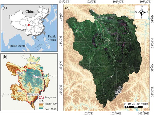
The Zoige wetland (32°10′–34°11′ N, 101°25′–103°17′ E) in the eastern Qinghai–Tibet Plateau (Figure 1) is the largest alpine wetland in China and was included in the list of wetlands of international importance in 1999. The region has an elevation from 3200 m to 4800 m and covers an area of approximately 22,177 km², including the partial regions of Maqu and Luqu of Gansu Province and Ruoergai, Hongyuan, and Aba of Sichuan Province. This area has a typical plateau semi-humid monsoon climate with an annual precipitation of 650 mm and an average temperature of 1.7°C (Cui et al. 2012).

Figure 1. (a) Location of the Zoige wetland in China, (b) the boundary of the study area, (c) the true color composite image of the Landsat 8 OLI data of the whole study area

The alpine meadow is the most typical plant type in the Zoige wetland (Niu et al. 2014). The alpine meadow consists of multiple cold-resistant and mesophytic species dominated by Kobresia with weeds and sedges (http://www.nsii.org.cn/2017/home.php). The alpine meadow usually experiences the early growth stage to the last growth stage from June to September; it becomes frozen in November and thaws in the following March (Wang et al. 2012; Niu et al. 2016). Marsh is an important wetland landscape and is referred to as the intermittently inundated area populated by emergent aquatic graminoid plants (Warner and Rubec 1997). A novel marsh meadow community that shares characters of alpine meadow and marsh has recently emerged because of the changed soil moisture availability with increasing warm climates, suggesting a potential secondary succession trend (Ma, Zhou, and Du 2011; Li et al. 2015). The hygrophilous kobresia littledalei living under the waterlogged or damp soil conditions are the predominant species in marsh meadow (http://www.nsii.org.cn/2017/home.php).

2.2. Data

Three scenes of Landsat 8 OLI images with a path/row of 131/036, 131/037, and 131/038 were used in this study. The images were acquired on 15 July 2016, when alpine meadows were in the growth stage and marshes were wet. All images are available on the website of the United States Geological Survey (https://earthexplorer.usgs.gov/). Radiometric calibration and atmospheric correction were performed on the images to convert the satellite digital numbers to surface reflectance. The Fast Line-of-Sight Atmospheric Analysis of Spectral Hypercube (FLAASH) module in ENVI 5.3 was employed for the atmospheric correction step, where atmospheric model, aerosol model, and aerosol retrieval were, respectively, set as tropical, rural, and 2-Band (K-T). Different scenes of images were then mosaicked into one image using the seamless mosaic method. For image mosaicking, the histogram matching technique was utilized to correct color differences, and the pixels in effective overlapping regions between images were calibrated and blended with underlying scenes through the seam-line feathering. Finally, the mosaicked image was clipped by a mask of the study area. To avoid possible negative effects induced by the fusion of multispectral and panchromatic bands (Thomas et al. 2008; Palubinskas 2016), this study did not perform pan-sharpening for images.

2.2.1. Features

In the present study, 16 features associated with wetland cover types have been considered based on spectral characters, normalized difference ratios, textural information, and topographical factors (Table 1): (1) Multispectral features can increase our ability to recognize wetland communities, and seven bands (band 1–7: coastal, blue, green, red, NIR, SWIR1, SWIR2) of Landsat 8 data are used as spectral features. (2) Two important spectral indexes, namely, normalized difference vegetation index (NDVI) and normalized difference water index (NDWI), were then calculated to enhance the separability of vegetation and water areas. (3) We also consider texture metrics because of the advantages in understanding the information between spatial neighborhood locations. Six texture statistics from the gray level co-occurrence matrix (GLCM) have been extracted based on the first principal component of multispectral bands, and the textural measures derived include the mean (MEAN), homogeneity (HOMO), angular second moment (ASM), dissimilarity (DIS), entropy (ENTR), and variance (VAR) (Haralick, Shanmugam, and Shanmugam 1973). The texture features were computed for horizontal direction using 1 step with different moving window sizes (3 × 3, 7 × 7, 11 × 11, 15 × 15, 19 × 19, 23 × 23, 31 × 31, 51 × 51). The information gain ratio (IGR) method was used to evaluate the importance level of the texture features with different scales. After trial-and-error tests, the features with the size of 19 × 19 are adopted for further classification due to the highest IGR score (Supplementary Figure 1). (4) The elevation is employed as auxiliary data to represent the role of topography in wetland cover classification. The elevation layer was extracted from the fundamental digital elevation model (DEM) data with a resolution of 30 m (http://www.gscloud.cn).

Table 1. List of input features used for wetland cover classification. NDVI = normalized difference vegetation index, NDWI = normalized difference water index, MEAN = mean, HOMO = homogeneity, ASM = angular second moment, DIS = dissimilarity, ENTR = entropy, VAR = variance

Feature types	Features	Equation
Spectral features	Coastal, blue, green, red, NIR, SWIR1, SWIR2	-
Normalized difference ratios	NDVI	$\frac{NIR-red}{NIR+red}$
	NDWI	$\frac{green-NIR}{green+NIR}$
Textural features	MEAN	$\sum _{i=0}^{N-1}\sum _{j=0}^{N-1}i\times P\left(i,j\right)$
	HOMO	$\sum _{i=0}^{N-1}\sum _{j=0}^{N-1}\frac{P\left(i,j\right)}{1+{\left(i-j\right)}^2}$
	ASM	$\sum _{i=0}^{N-1}\sum _{j=0}^{N-1}P{\left(i,j\right)}^2$
	DIS	$\sum _{i=0}^{N-1}\sum _{j=0}^{N-1}P\left(i,j\right)\times \left|i-j\right|$
	ENTR	$-\sum _{i=0}^{N-1}\sum _{j=0}^{N-1}P\left(i,j\right)\times \mathrm{l}\mathrm{n}\left(P\left(i,j\right)\right)$
	VAR	$\sum _{i=0}^{N-1}\sum _{j=0}^{N-1}P\left(i,j\right)\times {\left(i-\mathrm{M}\mathrm{E}\mathrm{A}\mathrm{N}\right)}^2$
Topographical factors	Elevation	-

$N$ is the number of the gray levels; $P\left(i,j\right)$ is the normalized gray level value of the cell $\left(i,j\right)$ of the GLCM.

2.2.2. Wetland cover classes

To conduct wetland mapping for Zoige wetland, eight representative wetland cover types were identified (Cui et al. 2015; Hou et al. 2020) in combination with a classification criterion from the National Specimen Information Infrastructure (http://www.nsii.org.cn/2017/home.php). These land cover types include five wetland classes, namely, alpine meadow, marsh meadow, marsh, river and lake, and floodplain, and three non-wetland classes, namely, sediments, residential area, and bedrock. Detailed descriptions of each class corresponding to the RS interpretation signature are summarized in Table 2. Google Earth Engine provides high-resolution images across the study area. From Google Earth images, the reference data with geographic coordinate information were manually labeled using visual interpretation. A total of 959 reference samples were collected for the study area (Figure 2). The visual inspection of sample locations shows that they spatially span across the whole Zoige wetland area, which ensures a geographic variability for labeled classes.

Figure 2. Locations of reference samples in the study area and typical examples of wetland covers in the Landsat 8 OLI images. AM = alpine meadow, MM = marsh meadow, M = marsh, RL = river and lake, FP = floodplain, S = sediments, RA = residential area, BR = bedrock

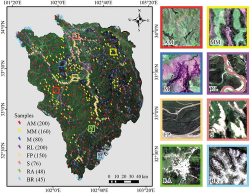
Table 2. Descriptions of wetland cover categories used in this study

Class name	Class code	Class description
Alpine meadow	AM	A vegetation community dominated by mesophytic Kobresia species
Marsh meadow	MM	Mixed areas of alpine meadow and marsh; characterized by rough texture
Marsh	M	Wet areas mainly consisting of emergent and submerged graminoid vegetation; displayed in deep violet under true color space
River and lake	RL	Permanent and seasonal water areas with the slim or elliptical shape; displayed in pink under true color space
Floodplain	FP	Periodically inundated areas; characterized by rough texture
Sediments	S	Sand land or deposits with high brightness
Residential area	RA	Regular shape with high brightness; usually distributed in low-elevation valleys
Bedrock	BR	Irregular shape with high brightness; usually exposed in ridges

3. Methodology

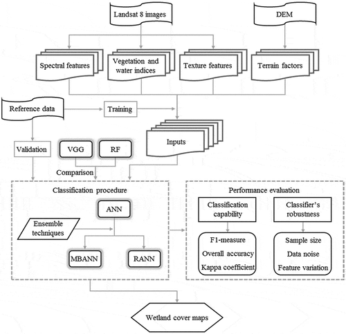
The wetland classification flowchart is shown in Figure 3. This study mainly consists of four steps: (1) data preparation and feature extraction; (2) implementation of the ANN, MBANN, and RANN; (3) evaluating the performance of classification methods, and (4) wetland cover mapping for the Zoige wetland.

Figure 3. The flowchart of wetland cover classification. ANN = artificial neural network, MBANN = MultiBoost artificial neural network, RANN = rotation artificial neural network, VGG = visual geometry group, RF = random forests

3.1. Classification methods

3.1.1. ANN

ANN is a highly interconnected architecture that attempts to simulate the operation mechanism of biological brains (Basheer and Hajmeer 2000). A typical multilayer-feedforward ANN consists of input, hidden, and output layers, and each layer is assigned with neurons used to process signals. During the feedforward stage, the signal is passed from the previous layer to the following layer via weight connection. The input to each neuron in the next layer is the weighted sum of all previously connected neurons. The neurons that receive input information are then transformed using an activation function (e.g. sigmoid function) to ensure the non-linear prediction. The learning procedure of ANN can be expressed as the following formula:

$\begin{array}{c}{y}_k=\phi \left(\sum _{j=1}^m{w}_{kj}\times x_j+b_k\right)\mathrm{\#}\left(1\right)\end{array}$

where $x_j$ and $w_{kj}$ respectively represent the $j$-th incoming neuron and its weight connected to the following $k$-th neuron, $b_k$ is the bias term, $\phi \left(.\right)$ denotes the activation function, and $y_k$ is the output.

In the backward learning phase, the error back propagation algorithm is adopted to adjust connected weights between neurons according to the discrepancy between computed and target values. The weights are iteratively updated until the error of the whole network meets a specified threshold or reaches the maximum cycle round.

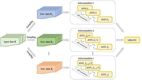
3.1.2. MultiBoost artificial neural network (MBANN)

The variance of a single learning algorithm can be reduced through successive iterations (Freund and Schapire 1996). However, the improvement in performance of the combination has a limitation as the sequent iteration round increases (Schapire et al. 1997). MultiBoost is an extended version of AdaBoost, which effectively mitigates the above problem (Webb 2000). Following the classical structure of ensemble classifiers (e.g. Bagging and AdaBoost), the MBANN method consists of the base-learner, served by ANN, and the ensemble scheme, served by MultiBoost (Figure 4). Instead of directly performing sequential iterations for base classifiers, MultiBoost defines subcommittees and an iterative termination mark variable $I_j$ ($j=1,2,\cdots ,\mathrm{\infty })$, where $j$-th subcommittee is a sub-decision group that contains $I_j$ AdaBoost-based ANNs. The value of $I_j$ specifies the iteration round at which the corresponding ($j$-th) subcommittee should terminate. Thus, $I_j$ determines the size of the subcommittee and follows the rules as follows:

$\begin{array}{c}{I}_j=\left\{\begin{array}{c}j\times \frac{T}{n},j=1,2,\cdots ,n\\ T,j=n,n+1,\cdots ,\mathrm{\infty }\end{array}\right.\mathrm{\#}\left(2\right)\end{array}$

Figure 4. Illustration of the MBANN method. ANN = artificial neural network, MBANN = MultiBoost artificial neural network, AB = AdaBoost

where $n$ is an integer with the value of $⌊\sqrt{T}⌋$. $T$ is the total number of iterations (also the total number of ANNs in the base-learning level).

Suppose the wetland classification dataset $\mathrm{D}=\left\{\mathbf{X},\mathbf{Y}\right\}={\left\{\left(x_i,y_i\right)\right\}}_{i=1}^m$ contains $\mathrm{m}$ instances, $\mathbf{X}$ and $\mathbf{Y}$ respectively denote the feature space and wetland cover categories. The construction of each subcommittee starts by sampling the original dataset into several subsets using continuous Poisson distribution. The sampling procedure is similar with the Bagging (Bauer and Kohavi 1999). Each subcommittee performs specified rounds of AdaBoost iterations for training ANNs using the corresponding sampled dataset. The sampled dataset is noted as ${\mathrm{D}}_j^{\prime }$, which is used for building the corresponding ($j$-th) subcommittee. For a subcommittee (e.g. $j=1$), a series of AdaBoost-based ANN is trained as the iteration round $t\left(t=1,2,\cdots ,T\right)$ increases.

$\begin{array}{c}{c}_t=ANN\left({\mathrm{D}}_j^{\prime }\right)\mathrm{\#}\left(3\right)\end{array}$

Before the iteration, the original dataset $\mathrm{D}$ is assigned by an initial weight for each instance $x_i$.

$\begin{array}{c}\omega \left(x_i\right)=\frac{1}{\mathrm{m}}i=1,2,\cdots ,m\mathrm{\#}\left(4\right)\end{array}$

When a subcommittee starts to perform successive iterations, the learning error ${\epsilon }_t$ and the weight ${\alpha }_t$ of $c_t$ in $t$-th iteration round are respectively estimated as the following formulas:

${\epsilon }_t=\sum i=1{\omega }_t\left(x_i\right)I\left(c_t\left(x_i\right)\ne y_i\right)\mathrm{\#}\left(5\right)$

$\begin{array}{c}{\alpha }_t=log\frac{1-{\epsilon }_t}{{\epsilon }_t}\mathrm{\#}\left(6\right)\end{array}$

where $I\left(.\right)$ is the indicator function.

After completing an iteration in a subcommittee, the weight of ${\mathrm{D}}_j^{\prime }$ is adjusted following the performance of previous-round ANN. Correctly classified instances will gain lower weights, whereas these misclassified instances with increased weights raise more attention by following-round ANNs. The weight of the ${\mathrm{D}}_j^{\prime }$ is updated as follows:

$\begin{array}{c}{\omega }_{t+1}\left(x_i\right)=\frac{{\omega }_t\left(x_i\right)}{Z_t}\times \{\begin{array}{c}2{\epsilon }_t\hspace{0.17em}if\hspace{0.17em}{c}_t\left(x_i\right)\ne y_i\\ 2\left(1-{\epsilon }_t\right)\hspace{0.17em}if\hspace{0.17em}{c}_t\left(x_i\right)=y_i\end{array}\mathrm{\#}\left(7\right)\end{array}$

where $Z_t$ is a normalization factor used to standardize ${\omega }_{t+1}\left(x_i\right)$.

The above procedure is repeated until the iteration termination condition ($t=I_j$) is met. That is, the $j$-th subcommittee is successfully formed and stops the intra AdaBoost iteration program. After that, the dataset ${\mathrm{D}}_{j+1}^{\prime }$ is employed, and the same procedure is performed for the next $\left(j+1\right)$-th subcommittee until the iteration cycle reaches $T$. Therefore, the MBANN is a composite model obtained from multiple iteration calculations of the ANNs. The final decision is made by the weighted voting of the predictions of all ANNs in different subcommittees, and the predictions of each subcommittee include all categories.

The prediction of the MBANN is involved in every ANNs and their corresponding weights:

$\begin{array}{c}C\left(x\right)=argma{x}_y\sum _{t=1}{\alpha }_{t}I\left(c_t\left(x\right)=y\right)\mathrm{\#}\left(8\right)\end{array}$

3.1.3. Rotation artificial neural network (RANN)

Constructing different feature spaces to train the learning algorithm is an effective way to perform ensemble classification (Polikar 2006). In this study, the construction of RANN is inspired by the rotation forests algorithm (Rodríguez, Kuncheva, and Alonso 2006), which produces composite ANNs based on a feature reconstruction scheme (Figure 5). Feature reconstruction processing aims to maximize the diversity of base-level ANNs and improve the information representation capability of original features. Therefore, the core idea of the algorithm is to create a sparse rotation matrix used to rotate the space of the original dataset.

Figure 5. Illustration of the RANN method. ANN = artificial neural network, RANN = rotation artificial neural network, PCA = principal component analysis

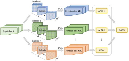
Given the dataset $\mathrm{D}=\left\{\mathbf{X},\mathbf{Y}\right\}={\left\{\left(x_i,y_i\right)\right\}}_{i=1}^m$ with $m$ numbers of instances and $n$ dimensions of feature set $\mathrm{F}$, where $\mathbf{Y}$ denotes wetland cover classes. Let $t=\left\{1,2,\cdots ,T\right\}$ represent the iteration round. The corresponding-round ANN is denoted as $c_t$.

First, subsets with different feature spaces are constructed from the original dataset. Specifically, for each iteration, the $\mathrm{F}$ is randomly split into $K$ disjoint subsets, and each subset contains $M=\mathrm{n}/K$ features. In $t$-th iteration round, the $j$-th feature subset with corresponding instances is used to compose a training set ${\mathbf{X}}_{t,j}$. To increase the diversity between training sets, a certain percentage (e.g. 75%) of ${\mathbf{X}}_{t,j}$ is selected to form a new set ${\mathbf{X}}_{t,j}^{\prime }$ by using the bootstrap sampling strategy.

Next, the sparse rotation matrix is constructed based on the principal component analysis (PCA) to transform the original data space. The purpose of PCA is not for dimensionality reduction but the rotation of the axes. Therefore, all principal components of ${\mathbf{X}}_{t,j}^{\prime }$ are retained to keep original data dimensions. The principal component coefficients of each ${\mathrm{X}}_{t,j}^{\prime }$ are calculated by PCA to form the corresponding sparse matrix in $t$-th iteration round. All principal component coefficients are stored in an eigenvector $V_{t,j}=\left[v_{t,j}^1,v_{t,j}^2,\cdots ,v_{t,j}^M\right]$, which is obtained from the following formula:

$\begin{array}{c}{\mathbf{X}}_{t,j}^{\prime }{\left({\mathbf{X}}_{t,j}^{\prime }\right)}^{\mathbf{T}}{V}_{t,j}=\lambda V_{t,j}\mathrm{\#}\left(9\right)\end{array}$

where ${\mathbf{X}}_{t,j}^{\prime }{\left({\mathbf{X}}_{t,j}^{\prime }\right)}^{\mathbf{T}}$ is the covariance matrix of ${\mathbf{X}}_{t,j}^{\prime }$ after being standardized by average values. $\lambda$ is the eigenvalue of ${\mathbf{X}}_{t,j}^{\prime }{\left({\mathbf{X}}_{t,j}^{\prime }\right)}^{\mathbf{T}}$.

The sparse rotation matrix ${\mathbf{R}}_t$ in $t$-th round is formed by placing $V_{t,j}$ on the main diagonal of a zero matrix:

$\begin{array}{rl}& {\mathbf{R}}_t=\left[v_{t,1}^1,v_{t,1}^2,\cdots ,v_{t,1}^M\right]\left[0\right]\left[0\right]\left[0\right]\\ & \left[v_{t,2}^1,v_{t,2}^2,\cdots ,v_{t,2}^M\right]\left[0\right]\cdots \left[0\right]\left[0\right]\\ & \left[v_{t,j}^1,v_{t,j}^2,\cdots ,v_{t,j}^M\right]\mathrm{\#}\left(10\right)\end{array}$

Since the order of features is disorganized by the random split operation, ${\mathbf{R}}_t$ should be rearranged to ${\mathbf{R}}_t^{\prime }$ in accordance with the order of original features of $\mathbf{X}$. Based on the sparse rotation matrix ${\mathbf{R}}_t^{\prime }$, the original $\mathbf{X}$ is transformed as follows:

$\begin{array}{c}{\mathbf{X}}^{\prime }=X{\mathbf{R}}_t^{\prime }\mathrm{\#}\left(11\right)\end{array}$

Finally, ANN builds classification rules on each transformed data. After $T$ iterations, the composite RANN is constructed using the majority voting results of all component ANNs:

$\begin{array}{c}C\left(x\right)=argma{x}_y\sum _{t=1}I\left(c_t\left(x\right)=y\right)\mathrm{\#}\left(12\right)\end{array}$

3.2. Model training and parameter setting

The ANN and ensemble models are constructed in the training process to learn the rule of wetland cover classification. A 10-fold cross-validation technique is adopted to train the classifiers as it provides more solid modeling procedures and gives a lower estimation of variance. The dataset is randomly divided into 10 subsets with an equal size, of which one subset is prepared for model validation and the remaining parts are utilized for training. Parameter tuning is an essential part of the model training process and the choice of training parameters has a direct influence on classification performance. In this study, the parameters of the classifiers are optimized using the grid search method. Each point in the grid consisted of possible combinations of predefined parameters is repeatedly tested and the model with the highest accuracy is selected as the optimum one. To train ANN for wetland classification, an ANN structure with one hidden layer that contains 12 nodes is used. The most important parameters for ANN are the learning rate, the momentum, and the training steps. As the choice of excessively large number of training steps does not improve classification performance when generalization error meets the limitation, we fix the value of the training steps as 1000 and only adjust the learning rate and the momentum. By using the grid search method, the learning rate and the momentum are, respectively, taken as 0.4 and 0.7 for the ANN. In terms of the MBANN, the numbers of iterations and subcommittees are, respectively, set to 30 and 4 to integrate ANNs. As for the RANN, the number of sub-feature sets is adjusted to 4 for data rotation. The sampling percentage and iteration number are respectively set to 70% and 30. Moreover, two state-of-the-art methods, namely, the deep visual geometry group (VGG) (Simonyan and Andrew 2014) and the RF ensemble algorithm, were implemented for comparison with our methods. The VGG11 consists of eight convolution layers with different convolution kernel sizes, three full connection layers, and a soft-max classifier. We tune the parameters for the deep learning model VGG11 empirically. Finally, a batch size of 50, an epoch of 30, an initial learning rate of 0.001, and a decay rate of 0.1 per 800 iterations are chosen for full-training VGG11. To perform wetland cover mapping using the VGG11, the whole image was decomposed into overlapped patches with 32 × 32 sizes. The class label that belongs to the patch is assigned to the center pixel of the patch. The RF is a popular classifier and achieves the ensemble of DTs. We attempt the numbers of DTs from 10 to 1000 in the training phase and finally set the number of DTs and the size of sub-feature sets as 700 and 4 for the RF algorithm.

3.3. Performance evaluation criteria

Classification capability is probably the most concerning aspect of performance for an algorithm. Classification capability can be measured using statistical indexes, such as overall accuracy (OA), Kappa coefficient (K), user’s accuracy (UA), producer’s accuracy (PA), class F1-score (F), and weighted F1-score (WF) (Zhang et al. 2019; Pouliot et al. 2019). OA is the ratio of correctly classified instances in the whole samples. K is an important indicator used to quantify the level of consistency between reference and predicted results. UA and PA denote the correct percentage for each class associated with predicted and reference results, respectively. F is a summary measure of the UA and PA for each class, formulated as $2\times \left(\mathrm{U}\mathrm{A}\times \mathrm{P}\mathrm{A}\right)/\left(\mathrm{U}\mathrm{A}+\mathrm{P}\mathrm{A}\right)$. WF denotes the sum of the class F-scores multiplied by the proportion of corresponding classes. Statistical significance of differences between the ensemble methods and benchmark methods in classification accuracy was evaluated using the pairwise z-score test (Congalton, Oderwald, and Mead 1983). The z score with a value greater than 1.96 indicates a statistically significant difference at the 5% level.

Robustness is another important property that should be considered for a classifier. In practical classification tasks, the field collection of reference data is usually constrained by labor and cost, especially for large-scale and remote areas that have limited access, such as Zoige wetland. Obtaining sufficient and comprehensive samples for calibrating classifiers is usually difficult. Although the manual labeled method based on high-resolution images or Google Earth is efficient, this method and a field survey are likely to suffer from data noise because of limited domain knowledge or human mistakes when conducting wetland class recognition and data processing (Dubeau et al. 2017; Di Vittorio and Georgakakos 2018). Furthermore, the feature extraction program varies from person to person. The use of different features generates different classification rules and causes variations in classification accuracy. Therefore, the algorithm utilized to classify wetland cover types should ideally be robust to those negative or dynamic factors to maintain classification performance. In this study, the robustness over sample size, data noise, and feature variation was tested for classifiers. The impacts of sample size on the classification accuracy were tested by decreasing the sample size from 100% to 20% in a decrement of 10%. Similarly, the evaluation of sensitiveness to data noise was performed by randomly mislabeling a specified ratio of training instances from 0% to 60% in an increment of 10%. Thus, the original label is randomly replaced by an incorrect label for a certain ratio of samples. Considering high noise level (>60%) is unlikely to arise in practical applications, the robustness test at this level is not performed. The feature variability effect was studied by randomly eliminating features from the initial feature set one by one. This procedure was repeated 10 times to mitigate the impacts of potential correlations between features, and the average value of accuracy was used for each round. The VGG11 is not included in this test because it is an end-to-end feature learning model that does not rely on handcrafted features. The standard deviation of the accuracy values was used to qualify the classifier’s sensitiveness to these variations, and a smaller standard deviation indicates better stability.

4. Results

4.1. Classification accuracy

Classification accuracies of various methods have been summarized in Table 3. WF, OA, and K give an overall evaluation on classification accuracies. The results consistently show that the RANN achieves the optimal classification performance, which gains the WF, OA, and K with values of 0.962, 0.961, and 0.954, respectively. The MBANN takes the second place, yielding the WF, OA, and K values of 0.942, 0.942, and 0.931, respectively. VGG11 is slightly behind the MBANN, yielding the WF, OA, and K values of 0.934, 0.934, and 0.922, respectively, followed by the RF, yielding the WF, OA, and K values of 0.931, 0.931, and 0.918, respectively. The classification accuracy obtained by the ANN is the lowest in comparison with other methods, yielding the above indexes with values of 0.915, 0.916, and 0.900, respectively.

Table 3. Classification accuracy evaluation and comparison of various classification methods. ANN = artificial neural network, MBANN = MultiBoost artificial neural network, RANN = rotation artificial neural network, VGG11 = visual geometry group, RF = random forests. AM = alpine meadow, MM = marsh meadow, M = marsh, RL = river and lake, FP = floodplain, S = sediments, RA = residential area, BR = bedrock

Classes	ANN			MBANN			RANN			VGG11			RF
	UA	PA	F	UA	PA	F	UA	PA	F	UA	PA	F	UA	PA	F
AM	0.930	0.930	0.930	0.964	0.925	0.944	0.969	0.950	0.960	0.939	0.967	0.953	0.935	0.935	0.935
MM	0.811	0.888	0.848	0.826	0.919	0.870	0.872	0.938	0.904	0.944	0.958	0.951	0.870	0.919	0.894
M	0.975	0.975	0.975	0.976	1.000	0.988	0.988	1.000	0.994	0.990	1.000	0.995	0.949	0.938	0.943
RL	0.955	0.960	0.958	0.995	0.990	0.992	1.000	1.000	1.000	0.923	0.904	0.914	0.961	0.975	0.968
FP	0.930	0.887	0.908	0.957	0.887	0.920	0.957	0.900	0.928	0.934	0.867	0.899	0.937	0.887	0.911
S	0.905	1.000	0.950	0.927	1.000	0.962	0.987	1.000	0.993	0.946	0.957	0.951	0.923	0.947	0.935
RA	0.971	0.708	0.819	0.951	0.813	0.876	1.000	0.958	0.979	0.823	0.879	0.850	0.915	0.896	0.905
BR	0.902	0.822	0.860	0.978	1.000	0.989	0.978	1.000	0.989	0.930	0.964	0.946	1.000	0.911	0.953
Overall evaluation	WF	OA	K	WF	OA	K	WF	OA	K	WF	OA	K	WF	OA	K
	0.915	0.916	0.900	0.942	0.942	0.931	0.962	0.961	0.954	0.934	0.934	0.922	0.931	0.931	0.918

A more detailed evaluation for per class can be inspected through the UP, PA, and F indexes. We may see that all methods are successful in classifying wetland cover classes except that the PA of the residential area for the ANN is lower than 0.8. The RANN can correctly classify wetland classes with F measures more than 0.9. Furthermore, the RANN has the highest accuracy indexes for the river and lake, and the floodplain. The VGG11 shows great advantages in classifying the marsh meadow and marsh, yielding UP, PA, and F values that exceed 0.94. The MBANN is also useful in discriminating the marsh, the river and lake, and the floodplain. However, the classification of the marsh meadow seems to present divergences as most of the classifiers (except the VGG11) have the lowest F measure on this wetland category. With respect to non-wetland classes, the residential area is usually misclassified by the ANN, MBANN, and the VGG11 because some confusions may exist between the residential area and sediments. The RANN achieves the highest discriminating power for the residential area, sediments, and bedrock, improving its overall classification accuracy substantially. In contrast, remaining classifiers are less effective at separating non-wetland classes. Thus, for most of the classifiers, the overall classification error is induced mainly by the marsh meadow or residential area being identified as wrong classes. By comparison, the RANN achieves favorable performance with a comprehensive ability to correctly classify wetland classes and non-wetland classes, whose accuracies are constantly greater than 0.9 in all cases. It is worth mentioning that ensemble methods usually have a better per-class estimation against the single ANN. For instance, the per-class F is improved by 1.2–12.9% and 1.9–16.0% by using the MBANN and RANN models. The results demonstrate the advantages of using ensemble learning techniques in classifying wetland covers.

Significance test results (Table 4) show that the z-scores of pairs of ANN-RF and ANN-VGG11 are smaller than 1.96. This indicates the classification result produced by the ANN is similar with the RF and VGG11, and thus failing to reject the null hypothesis. For the remaining comparative pairs, their z-scores exceed the significance-level threshold, meaning that they are significantly different in statistics thereby rejecting the null hypothesis.

Table 4. Z-score test with associated probability value (P) for model pairs. ANN = artificial neural network, MBANN = MultiBoost artificial neural network, RANN = rotation artificial neural network, VGG11 = visual geometry group, RF = random forests

Comparative pairs	z score	P value	Significance level
ANN vs. MBANN	3.273	0.001	Yes
ANN vs. RANN	4.041	0.000	Yes
ANN vs. RF	0.962	0.336	No
ANN vs. VGG11	0.283	0.777	No
MBANN vs. RANN	2.121	0.034	Yes
MBANN vs. RF	2.500	0.012	Yes
MBANN vs. VGG11	2.082	0.037	Yes
RANN vs. VGG11	3.413	0.001	Yes
RANN vs. RF	3.771	0.000	Yes

4.2. Wetland cover classification

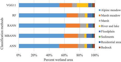
All methods are used to develop the wetland cover maps for the Zoige wetland, and the results are displayed in Figure 6. All methods seem to agree in the allocation of wetland cover types in most cases. Detailed area percentages of wetland cover categories are given in Figure 7. Within the wetland classes, the alpine meadow occupies the largest area and is widely distributed across the region with area percentages from 53% to 63%. Most classifiers allocate the marsh meadow with area proportions ranging from 15.04% to 18.18%, but more areas (24.62%) are predicted by the ANN model. A significant discrepancy also exists in the assignment of the river and lake. A high percentage of 14.89% is assigned to this class by using the VGG11, whereas remaining classifiers have a similar percentage with ranges from 2.61% to 3.45%. Apart from these differences, consistent results are also derived, for example, the marsh and floodplain account for 6.33–9.05% and 4.13–6.15% of the total area, respectively. Together, these classes occupy 94.94–96.48% of the total Zoige wetland area. The remaining non-wetland classes, such as the sediments, residential area, and bedrock, are sparsely distributed in the terrestrial land and account for only 3.12% to 5.06%.

Figure 6. Wetland cover maps obtained by the five classifiers: (a) artificial neural network, (b) MultiBoost artificial neural network, (c) rotation artificial neural network, (d) visual geometry group, and (e) random forests

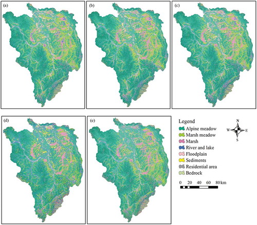
Figure 7. Area percentages of wetland cover classes predicted by different classification methods. ANN = artificial neural network, MBANN = MultiBoost artificial neural network, RANN = rotation artificial neural network, VGG11 = visual geometry group, RF = random forests

4.3. Robustness analysis

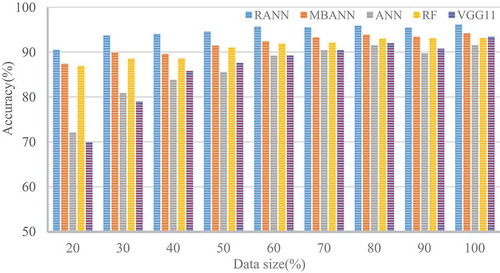
The influence of the data size, data noise, and feature variation on classification performances has been tested for various classifiers. For the data size test, the overall accuracy values of all methods show a downward trend with the decrease in data size from 100% to 20%, with decrements of 19.45%, 6.79%, 5.52%, 23.24%, and 6.28% for ANN, MBANN, RANN, VGG11, and RF, respectively (Figure 8). The ANN-based ensemble methods outperform single ANN for different data sizes, with accuracy increases of approximately 2.34–15.26% for the MBANN and 4.30–18.42% for the RANN. Also, the accuracies of the MBANN and RANN are consistently better than the VGG11 and RF. The two ANN-based ensemble classifiers have accuracy values higher than 90% when at least 50% of the original data is used. The ANN and VGG11 yield accuracy values lower than 80% when the data size remains at only 20%. The RANN gains the lowest standard deviation of accuracy with a value of 1.65, followed by the MBANN (2.20), RF (2.21), ANN (6.05), and VGG11 (7.07). These results connote that two ANN-based ensemble methods are insensitive to the variation of data size and can help the ANN to mitigate the negative impact of insufficient data on classification accuracy. The RF and the MBANN perform comparably without appreciable differences in robustness to data size, while the VGG11 is particularly sensitive to the reduction in data size and requires substantial samples to maintain classification ability.

Figure 8. Robustness evaluation concerning the impact of the data size on the classification accuracy of classifiers. RANN = rotation artificial neural network, MBANN = MultiBoost artificial neural network, ANN = artificial neural network, RF = random forests, VGG11 = visual geometry group

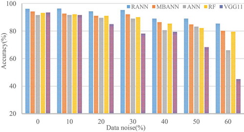
In terms of the data noise test, all classification methods present a decreasing trend in accuracy with an increase in data noise from 0% to 60% (Figure 9). The lowest accuracy is obtained for all methods when data noise goes up to 60%. The ANN-based ensemble methods can resist the low-moderate level of noise and exhibit a preferable classification capability than the ANN, RF, and VGG11 for all cases. Particularly, the RANN holds constant classification accuracy (>94%) as the noise level increases to 30%, which is comparable to the case when the noise is not introduced. The VGG11 does not perform well with noise data because its accuracy starts to decline rapidly when the noise exceeds 10%. The overall fluctuation in accuracy values is measured using the standard deviation, with the values of 4.03, 4.74, 4.90, 8.50, and 15.30 being obtained for the RANN, MBANN, RF, ANN, and VGG11, respectively. The RANN is found to be least affected by data noise, while the VGG11 has the worst stability in this case.

Figure 9. Robustness evaluation concerning the impact of the data noise on the classification accuracy of classifiers. RANN = rotation artificial neural network, MBANN = MultiBoost artificial neural network, ANN = artificial neural network, RF = random forests, VGG11 = visual geometry group

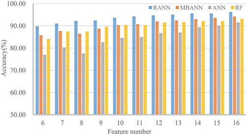
With respect to the influence of feature variability, the accuracies of all methods reduce in a nearly linear tendency after a certain number of features being randomly removed from the initial feature set (Figure 10). Similarly, the RANN consistently exhibits a superior classification capability to the MBANN, ANN, and RF. After nine features are eliminated, the accuracy of the RANN remains on a high level with a value greater than 90%. By contrast, the accuracy declines by approximately 14% for ANN when half of the features are not used. As the features were gradually removed from classification programs, the RANN and MBANN constantly improve the classification accuracy of the ANN with an increase of 2.61–8.72% and 4.59–12.78%, respectively. It should be noticed that the RF is also robust to feature variation with an accuracy decrement of no more than 10%. Among the classifiers, RANN gains the lowest standard deviation of accuracy with the value of 1.96, followed by the RF (2.56), MBANN (2.78), and ANN (4.67). Again, ensemble techniques successfully reinforce the classification stability of the ANN, and the RANN exhibits the best robustness. However, the RF has a comparable and low standard deviation, connoting that the RF was equally insensitive to feature variations in comparison with the MBANN.

Figure 10. Robustness evaluation concerning the impact of the feature variation on the classification accuracy of classifiers. RANN = rotation artificial neural network, MBANN = MultiBoost artificial neural network, ANN = artificial neural network, RF = random forests

5. Discussion

Developing large-scale and high-precision wetland mapping products that conform to domain knowledge to characterize the unique wetland landscapes is of significance for wetland monitoring and management. Currently, the need for more valuable and reliable wetland cover classification results and the fact that wetland classification from the RS perspective still faces challenges portend a necessity to explore novel and effective classification methods. Ensemble learning is an important branch of the machine learning, whose contribution has been well documented in a variety of disciplines, such as landslide susceptibility mapping (Hu et al. 2020, 2021), flood susceptibility modeling (Chen et al. 2019), and credit scoring analysis (Wang et al. 2011). However, the exploration and application of ensemble algorithms for wetland studies are relatively limited. In this study, we applied two different ANN-based ensemble methods, namely, the RANN and MBANN, to address real-world wetland classification problems and provide an improved classification scheme. The Zoige wetland sited in the Qinghai–Tibet Plateau is taken as the case study area. We expect that the use of ensemble techniques could provide improved performance against the single ANN and construct reliable wetland classification programs, and the resultant maps by ensemble predictions can be used to monitory wetland cover for the Zoige region.

Our results show that the ANN-based ensemble technique is more powerful in classifying wetland covers with RS images when compared with the single ANN, RF, and VGG11. However, different methods have different advantages in recognizing wetland cover classes. For example, the RF holds the best UA for the bedrock, and the VGG11 is particularly good at distinguishing the alpine meadow, marsh meadow, and marsh. In most cases, the single ANN underperforms the RF and VGG11. It should be noted that ensemble learning techniques lead to an improved overall estimation for individual classes (e.g. per-class F measure) over the ANN, even for the classes that are easily misclassified (e.g. marsh meadow and residential area). We may see that the ANN with ensemble classifications presents better per-class F measures than the VGG11 and RF, and this ensures the improvement in overall classification ability. With the RANN, the WF, OA, and K are respectively improved by 4.7%, 4.5%, and 5.4% over the ANN. For the MBANN, the above indexes are 2.7%, 2.6%, and 3.1% better than the ANN. Related studies have well summarized the reasons why the classification capability of an ensemble is stronger than that of the corresponding components (Dietterich 2000; Zhou 2009): (1) the search processes of a single learner may be imperfect, and the ensemble that performs the search processes from different initial points possibly provides a better approximation to the objective function than any of the single learners; (2) the hypothesis space being searched may not contain the true target function, while ensembles are able to expand the hypothesis space to make a good approximation. The RANN method benefits from the rotation mechanism that can maximize the diversity of the ANNs and extract useful and discriminative information from the original feature space (Rodríguez, Kuncheva, and Alonso 2006), enabling the RANN to take advantage of diverse ANNs to achieve a good approximation to the true fitting function. Additionally, Eeti and Buddhiraju (2019) have summarized that using the ANN with rotation forest effectively mitigates replication problem, fragmentation problem, and myopic problem. Unlike the RANN, the MBANN is the ensemble developed from the sequential iteration in combination with the parallel sampling technique, which is still seldom investigated in the wetland cover classification field. MultiBoost is skillful in reducing the variance and bias of the component algorithm (Zhu et al. 2018). This property helps the MBANN to derive an improved classification capability against the ANN. In contrast to the revealed research that deep learning models are superior to shallow-structure approaches (Mahdianpari et al. 2018b; DeLancey et al. 2019), our RANN and MBANN do outperform the VGG11. The findings are similar to those of Jozdani, Johnson, and Chen (2019), who reported that some ensemble learning algorithms (e.g. RF, GBT, and XGB) are likely to produce better classification results than deep CNN. The results connote that shallow learning methods can be boosted by the stacking of proper ensemble techniques to yield comparable classification accuracy to the state-of-the-art methods.

Another contribution of our study is the evaluation of the stability of classification methods when wetland classification is the case. In RS applications, collecting a large amount of labeled data for each category may be difficult and noise prone (Jozdani, Johnson, and Chen 2019). Furthermore, the selection of features for RS classification depends on the individual experience and knowledge, which directly influences the quality of the final classification results (Cordeiro and Rossetti 2015). Thus, we always expect applied algorithms to keep favorable adaptability and consistent classification accuracy even if negative or dynamic factors are encountered. In this study, the robustness evaluation shows that the RANN and MBANN are insensitive to data size, data noise, and feature variation. Ensemble techniques can help single ANN to maintain classification accuracy by better dealing with the limited data size, data noise, and feature variation. Particularly, the RANN exhibits the best robustness, with the lowest standard deviation of accuracy on average. These properties of ensemble methods may help classification algorithms to keep uniformity in classification capability when the scenery changes. By comparison, the VGG11 fails to remain stable with the decrease in data size. The performance of deep learning methods depends greatly on sample numbers (Jozdani, Johnson, and Chen 2019). The limited number of training samples constrains the effectiveness of deep learning methods due to the overfitting problem (Mahdianpari et al. 2018a). Additionally, the VGG11 is sensitive to the data noise because its accuracy substantially reduces by more than 45% when the noise level goes up to 60%. The possible reason is that the powerful fitting abilities force the VGG11 to focus on the incorrect classes thereby obtaining poor generalization performance. In this regard, ensemble learning methods can boost classification robustness and provide a promising solution to overcome the hardship from limited data information, data noise, and feature variability for wetland classification.

Model selection subjectively relies on the perspective of the users in specific circumstances. The efficiency of a classifier is also important for wetland mapping. A possible limitation of the ensemble classifications is that the improvement in classification performance needs more computational burden. The RANN (192.6 s) and MBANN (19.8 s) take extra computation times than the single ANN (6.5 s) in the modeling process. By comparison, the RF (7.6 s) as an ensemble method is more easily implemented. Nevertheless, the two ANN-based ensemble methods are more efficient than the VGG11 because the training procedure of the latter is quite time-consuming (18,139.2 s). We argue that the two ANN-based ensemble methods have an acceptable computation burden, which are still effective in practical wetland cover classification tasks.

6. Conclusion

Exploration with effective schemes to improve the performance of classification methods is critical to guarantee the quality of wetland classification products. Machine learning algorithms may suffer from insufficient classification ability and poor stability because of inherent factors (e.g. single fitting function and shallow structure) and external factors (e.g. limited training data, bad-quality data, and variability in feature selection), which restrict their applicability in wetland cover classification. In this study, we attempted to couple the single ANN with two ensemble techniques to construct the MBANN and RANN, and explored their potential and values in wetland classification by taking the Zoige wetland as the case area. The ensemble classification has the following attractive advantages: (1) Per-class accuracy can be refined by using the RANN and MBANN. This property leads to a significant improvement in overall classification accuracy against the single ANN. (2) The RANN and MBANN outperform the VGG11 and RF concerning classification capability, demonstrating the potential of ensemble learning techniques in generating comparable classification accuracy to the state-of-the-art methods. (3) Ensemble methods can maintain stability for classification and refine individual classifiers by better handling limited data size, data noise, and feature variation in wetland classification.

This study emphasizes the important role of ensemble methods in building accurate and reliable wetland classification programs because ensemble methods can boost the single algorithm in classification capability and robustness. The RANN and MBANN provide a promising scheme for improved wetland classification. Particularly, the RANN exhibits optimal comprehensive performance.

In the future, more studies are needed to evaluate the spatial and temporal transferability of classification methods for wetland cover classification. Also, the effectiveness of the ensemble classification still needs to be tested in different cases.

Disclosure of potential conflicts of interest

No potential conflict of interest was reported by the author(s).

Acknowledgements

The authors are thankful to the National Key Research and Development Program of China [NQI-2018YFF0215003] and the Key Laboratory of Urban Land Resources Monitoring and Simulation, Ministry of Land and Resources for supporting this study. The authors are also deeply grateful to editors and reviewers for their valuable comments and suggestions, which help to improve this paper.

Additional information

Funding

This work was supported by the National Key Research and Development Program of China [Grant number: NQI-2018YFF0215003] and the project from the Key Laboratory of Urban Land Resources Monitoring and Simulation, Ministry of Land and Resources [Grant number: KF-2019-04-046].

References

- Adam, E., O. Mutanga, J. Odindi, and E. M. Abdel-Rahman. 2014. “Land-use/cover Classification in a Heterogeneous Coastal Landscape Using RapidEye Imagery: Evaluating the Performance of Random Forest and Support Vector Machines Classifiers.” International Journal of Remote Sensing 35 (10): 3440–3458. doi:10.1080/01431161.2014.903435.
- Adam, E., O. Mutanga, and D. Rugege. 2010. “Multispectral and Hyperspectral Remote Sensing for Identification and Mapping of Wetland Vegetation: A Review.” Wetlands Ecology and Management 18 (3): 281–296. doi:10.1007/s11273-009-9169-z.
- Amani, M., B. Salehi, S. Mahdavi, B. Brisco, and M. Shehata. 2018. “A Multiple Classifier System to Improve Mapping Complex Land Covers: A Case Study of Wetland Classification Using SAR Data in Newfoundland, Canada.” International Journal of Remote Sensing 39 (21): 7370–7383. doi:10.1080/01431161.2018.1468117.
- Amani, M., B. Salehi, S. Mahdavi, J. Granger, and B. Brisco. 2017. “Wetland Classification in Newfoundland and Labrador Using Multi-source SAR and Optical Data Integration.” GIScience & Remote Sensing 54 (6): 779–796. doi:10.1080/15481603.2017.1331510.
- Basheer, I. A., and M. N. Hajmeer. 2000. “Artificial Neural Networks: Fundamentals, Computing, Design, and Application.” Journal of Microbiological Methods 43 (1): 3–31. doi:10.1016/S0167-7012(00)00201-3.
- Bauer, E., and R. Kohavi. 1999. “An Empirical Comparison of Voting Classification Algorithms: Bagging, Boosting, and Variants.” Machine Learning 36 (1/2): 105–139. doi:10.1023/A:1007515423169.
- Breiman, L. 1996. “Bagging Predictors.” Machine Learning 24 (2): 123–140. doi:10.1007/BF00058655.
- Breiman, L. 2001. “Random Forest.” Machine Learning 45 (1): 5–32. doi:10.1023/A:1010933404324.
- Cai, Y., X. Li, M. Zhang, and H. Lin. 2020. “Mapping Wetland Using the Object-based Stacked Generalization Method Based on Multi-temporal Optical and SAR Data.” International Journal of Applied Earth Observation and Geoinformation 88: 92. doi:10.1016/j.jag.2020.102064.
- Chen, H., Q. Zhu, C. Peng, N. Wu, Y. Wang, X. Fang, Y. Gao, et al. 2013. “The Impacts of Climate Change and Human Activities on Biogeochemical Cycles on the Qinghai-Tibetan Plateau.” Global Change Biology 19 (10): 2940–2955. doi:10.1111/gcb.12277.
- Chen, W., H. Hong, S. Li, H. Shahabi, B. B. Ahmad, X. Wang, and B. B. Ahmad. 2019. “Flood Susceptibility Modelling Using Novel Hybrid Approach of Reduced-error Pruning Trees with Bagging and Random Subspace Ensembles.” Journal of Hydrology 575: 864–873. doi:10.1016/j.jhydrol.2019.05.089.
- Chen, Y., P. Dou, and X. Yang. 2017. “Improving Land Use/cover Classification with a Multiple Classifier System Using AdaBoost Integration Technique.” Remote Sensing 9 (10): 10. doi:10.3390/rs9101055.
- Congalton, R. G., R. G. Oderwald, and R. A. Mead. 1983. “Assessing Landsat Classification Accuracy Using Discrete Multivariate Analysis Statistical Techniques.” Photogrammetric Engineering and Remote Sensing 49 (12): 1671–1678.
- Cordeiro, C. L. D. O., and D. D. F. Rossetti. 2015. “Mapping Vegetation in a Late Quaternary Landform of the Amazonian Wetlands Using Object-based Image Analysis and Decision Tree Classification.” International Journal of Remote Sensing 36 (13): 3397–3422. doi:10.1080/01431161.2015.1060644.
- Cui, Q., X. Wang, C. Li, Y. Cai, Q. Liu, and R. Li. 2015. “Ecosystem Service Value Analysis of CO2 Management Based on Land Use Change of Zoige Alpine Peat Wetland, Tibetan Plateau.” Ecological Engineering 76: 158–165. doi:10.1016/j.ecoleng.2014.03.035.
- Cui, Q., X. Wang, D. Li, and X. Guo. 2012. “An Ecosystem Health Assessment Method Integrating Geochemical Indicators of Soil in Zoige Wetland, Southwest China.” Procedia Environmental Sciences 13: 1527–1534. doi:10.1016/j.proenv.2012.01.145.
- Dai, L., and C. Liu. 2010. “Multiple Classifier Combination for Land Cover Classification of Remote Sensing Image.” Paper presented at the Proceedings of the 2010 2nd International Conference on Information Science and Engineering (ICISE), Hangzhou, China, 4–6 December, 2010.
- DeLancey, E. R., J. F. Simms, M. Mahdianpari, B. Brisco, C. Mahoney, and J. Kariyeva. 2019. “Comparing Deep Learning and Shallow Learning for Large-scale Wetland Classification in Alberta, Canada.” Remote Sensing 12 (1): 1. doi:10.3390/rs12010002.
- Di Vittorio, C. A., and A. P. Georgakakos. 2018. “Land Cover Classification and Wetland Inundation Mapping Using MODIS.” Remote Sensing of Environment 204: 1–17. doi:10.1016/j.rse.2017.11.001.
- Dietterich, T. G. 2000. “An Experimental Comparison of Three Methods for Constructing Ensembles of Decision Trees: Bagging, Boosting, and Randomization.” Machine Learning 40 (2): 139–157. doi:10.1023/A:1007607513941.
- Dronova, I. 2015. “Object-based Image Analysis in Wetland Research: A Review.” Remote Sensing 7 (5): 6380–6413. doi:10.3390/rs70506380.
- Dubeau, P., D. King, D. Unbushe, and L.-M. Rebelo. 2017. “Mapping the Dabus Wetlands, Ethiopia, Using Random Forest Classification of Landsat, PALSAR and Topographic Data.” Remote Sensing 9 (10): 10. doi:10.3390/rs9101056.
- Duro, D. C., S. E. Franklin, and M. G. Dubé. 2012. “A Comparison of Pixel-based and Object-based Image Analysis with Selected Machine Learning Algorithms for the Classification of Agricultural Landscapes Using SPOT-5 HRG Imagery.” Remote Sensing of Environment 118: 259–272. doi:10.1016/j.rse.2011.11.020.
- Eeti, L. N., and K. M. Buddhiraju. 2019. “Two Hidden Layer Neural Network-based Rotation Forest Ensemble for Hyperspectral Image Classification.” Geocarto International 1: 1–18. doi:10.1080/10106049.2019.1678680.
- Fariba, M., S. Bahram, M. Masoud, M. Mahdi, and B. Brian. 2018. “An Efficient Feature Optimization for Wetland Mapping by Synergistic Use of Sar Intensity, Interferometry, and Polarimetry Data.” International Journal of Applied Earth Observation & Geoinformation 73: 450–462. doi:10.1016/j.jag.2018.06.005.
- Feng, M., J. O. Sexton, S. Channan, and J. R. Townshend. 2015. “A Global, High-resolution (30-m) Inland Water Body Dataset for 2000: First Results of A Topographic–spectral Classification Algorithm.” International Journal of Digital Earth 9 (2): 113–133. doi:10.1080/17538947.2015.1026420.
- Fluet-Chouinard, E., B. Lehner, L.-M. Rebelo, F. Papa, and S. K. Hamilton. 2015. “Development of a Global Inundation Map at High Spatial Resolution from Topographic Downscaling of Coarse-scale Remote Sensing Data.” Remote Sensing of Environment 158: 348–361. doi:10.1016/j.rse.2014.10.015.
- Franklin, S., and O. Ahmed. 2017. “Object-based Wetland Characterization Using Radarsat-2 Quad-Polarimetric SAR Data, Landsat-8 OLI Imagery, and Airborne Lidar-derived Geomorphometric Variables.” Photogrammetric Engineering & Remote Sensing 83 (1): 27–36. doi:10.14358/pers.83.1.27.
- Freund, Y., and R. E. Schapire. 1996. “Experiments with a New Boosting Algorithm.” In Thirteenth International Conference on ML, 148–156. Bari, Italy.
- Gallant, A. 2015. “The Challenges of Remote Monitoring of Wetlands.” Remote Sensing 7 (8): 10938–10950. doi:10.3390/rs70810938.
- Ghimire, B., J. Rogan, V. R. Galiano, P. Panday, and N. Neeti. 2013. “An Evaluation of Bagging, Boosting, and Random Forests for Land-cover Classification in Cape Cod, Massachusetts, USA.” GIScience & Remote Sensing 49 (5): 623–643. doi:10.2747/1548-1603.49.5.623.
- Glanz, H., L. Carvalho, D. Sulla-Menashe, and M. A. Friedl. 2014. “A Parametric Model for Classifying Land Cover and Evaluating Training Data Based on Multi-temporal Remote Sensing Data.” ISPRS Journal of Photogrammetry and Remote Sensing 97: 219–228. doi:10.1016/j.isprsjprs.2014.09.004.
- Gorham, E. 1991. “Northern Peatlands: Role in the Carbon Cycle and Probable Responses to Climatic Warming.” Ecological Applications 1 (2): 182–195. doi:10.2307/1941811.
- Gosselin, G., R. Touzi, and F. Cavayas. 2014. “Polarimetric Radarsat-2 Wetland Classification Using the Touzi Decomposition: Case of the Lac Saint-Pierre Ramsar Wetland.” Canadian Journal of Remote Sensing 39 (6): 491–506. doi:10.5589/m14-002.
- Halmy, M. W. A., and P. E. Gessler. 2015. “The Application of Ensemble Techniques for Land-cover Classification in Arid Lands.” International Journal of Remote Sensing 36 (22): 5613–5636. doi:10.1080/01431161.2015.1103915.
- Haralick, R. M., K. Shanmugam, and K. Shanmugam. 1973. “Textural Features for Image Classification.” IEEE Transactions on Systems, Man, and Cybernetics 3 (6): 610–621. doi:10.1109/TSMC.1973.4309314.
- Hong, S.-H., H.-O. Kim, S. Wdowinski, and E. Feliciano. 2015. “Evaluation of Polarimetric SAR Decomposition for Classifying Wetland Vegetation Types.” Remote Sensing 7 (7): 8563–8585. doi:10.3390/rs70708563.
- Hou, M., J. Ge, J. Gao, B. Meng, Y. Li, J. Yin, J. Liu, Q. Feng, and T. Liang. 2020. “Ecological Risk Assessment and Impact Factor Analysis of Alpine Wetland Ecosystem Based on LUCC and Boosted Regression Tree on the Zoige Plateau, China.” Remote Sensing 12 (3): 3. doi:10.3390/rs12030368.
- Hu, X., H. Mei, H. Zhang, Y. Li, and M. Li. 2021. “Performance Evaluation of Ensemble Learning Techniques for Landslide Susceptibility Mapping at the Jinping County, Southwest China.” Natural Hazards 105 (2): 1663–1689. doi:10.1007/s11069-020-04371-4.
- Hu, X., H. Zhang, H. Mei, D. Xiao, Y. Li, and M. Li. 2020. “Landslide Susceptibility Mapping Using the Stacking Ensemble Machine Learning Method in Lushui, Southwest China.” Applied Sciences 10 (11): 4016–4037. doi:10.3390/app10114016.
- Jozdani, S. E., B. A. Johnson, and D. Chen. 2019. “Comparing Deep Neural Networks, Ensemble Classifiers, and Support Vector Machine Algorithms for Object-based Urban Land Use/land Cover Classification.” Remote Sensing 11 (14): 14. doi:10.3390/rs11141713.
- Kesikoglu, M. H., U. H. Atasever, F. Dadaser-Celik, and C. Ozkan. 2019. “Performance of ANN, SVM and MLH Techniques for Land Use/cover Change Detection at Sultan Marshes Wetland, Turkey.” Water Science and Technology 80 (3): 466–477. doi:10.2166/wst.2019.290.
- Kumar, L., and P. Sinha. 2014. “Mapping Salt-marsh Land-cover Vegetation Using High-spatial and Hyperspectral Satellite Data to Assist Wetland Inventory.” GIScience & Remote Sensing 51 (5): 483–497. doi:10.1080/15481603.2014.947838.
- Lagos, N. A., P. Paolini, E. Jaramillo, C. Lovengreen, C. Duarte, and H. Contreras. 2008. “Environmental Processes, Water Quality Degradation, and Decline of Waterbird Populations in the Rio Cruces Wetland, Chile.” Wetlands 28 (4): 938–950. doi:10.1672/07-119.1.
- LeCun, Y., B. Boser, J. S. Denker, D. Henderson, R. E. Howard, W. Hubbard, and L. D. Jackel. 1989. “Backpropagation Applied to Handwritten Zip Code Recognition.” Neural Computation 1 (4): 541–551. doi:10.1162/neco.1989.1.4.541.
- Lei, G., A. Li, J. Bian, H. Yan, X. Nan, Z. Zhang, and X. Nan. 2020. “Oic-mce: A Practical Land Cover Mapping Approach for Limited Samples Based on Multiple Classifier Ensemble and Iterative Classification.” Remote Sensing 12 (6): 987–1008. doi:10.3390/rs12060987.
- Li, H., A. B. Nicotra, D. Xu, and G. Du. 2015. “Habitat-specific Responses of Leaf Traits to Soil Water Conditions in Species from a Novel Alpine Swamp Meadow Community.” Conservation Physiology 3 (1): 1–8. doi:10.1093/conphys/cov046.
- Liu, G. S., and G. X. Wang. 2018. “Influence of Short-term Experimental Warming on Heat-water Processes of the Active Layer in a Swamp Meadow Ecosystem of the Qinghai-Tibet Plateau.” Sciences in Cold and Arid Regions 8 (2): 125–134. doi:10.3724/SP.J.1226.2016.00125.
- Ma, M., X. Zhou, and G. Du. 2011. “Soil Seed Bank Dynamics in Alpine Wetland Succession on the Tibetan Plateau.” Plant and Soil 346 (1–2): 19–28. doi:10.1007/s11104-011-0790-2.
- Mahdavi, S., B. Salehi, J. Granger, M. Amani, B. Brisco, and W. Huang. 2017. “Remote Sensing for Wetland Classification: A Comprehensive Review.” GIScience & Remote Sensing 55 (5): 623–658. doi:10.1080/15481603.2017.1419602.
- Mahdianpari, M., B. Salehi, F. Mohammadimanesh, S. Homayouni, and E. Gill. 2018a. “The First Wetland Inventory Map of Newfoundland at a Spatial Resolution of 10 M Using Sentinel-1 and Sentinel-2 Data on the Google Earth Engine Cloud Computing Platform.” Remote Sensing 11 (1): 1. doi:10.3390/rs11010043.
- Mahdianpari, M., B. Salehi, F. Mohammadimanesh, and M. Motagh. 2017. “Random Forest Wetland Classification Using ALOS-2 L-band, RADARSAT-2 C-band, and TerraSAR-X Imagery.” ISPRS Journal of Photogrammetry and Remote Sensing 130: 13–31. doi:10.1016/j.isprsjprs.2017.05.010.
- Mahdianpari, M., B. Salehi, M. Rezaee, F. Mohammadimanesh, and Y. Zhang. 2018b. “Very Deep Convolutional Neural Networks for Complex Land Cover Mapping Using Multispectral Remote Sensing Imagery.” Remote Sensing 10 (7): 7. doi:10.3390/rs10071119.
- Mohammadimanesh, F., B. Salehi, M. Mahdianpari, M. Motagh, and B. Brisco. 2018. “An Efficient Feature Optimization for Wetland Mapping by Synergistic Use of SAR Intensity, Interferometry, and Polarimetry Data.” International Journal of Applied Earth Observation and Geoinformation 73: 450–462. doi:10.1016/j.jag.2018.06.005.
- Niu, B., Y. He, X. Zhang, G. Fu, P. Shi, M. Du, Y. Zhang, and N. Zong. 2016. “Tower-based Validation and Improvement of MODIS Gross Primary Production in an Alpine Swamp Meadow on the Tibetan Plateau.” Remote Sensing 8 (7): 7. doi:10.3390/rs8070592.
- Niu, K., P. Choler, F. De Bello, N. Mirotchnick, G. Du, and S. Sun. 2014. “Fertilization Decreases Species Diversity but Increases Functional Diversity: A Three-year Experiment in A Tibetan Alpine Meadow.” Agriculture, Ecosystems & Environment 182: 106–112. doi:10.1016/j.agee.2013.07.015.
- Nogueira, K., O. A. B. Penatti, and J. A. D. Santos. 2017. “Towards Better Exploiting Convolutional Neural Networks for Remote Sensing Scene Classification.” Pattern Recognition 61: 539–556. doi:10.1016/j.patcog.2016.07.001.
- Palubinskas, G. 2016. “Model-based View at Multi-resolution Image Fusion Methods and Quality Assessment Measures.” International Journal of Image & Data Fusion 7 (3): 203–218. doi:10.1080/19479832.2016.1180326.
- Poiani, K. A., W. Carter Johnson, G. A. Swanson, and T. C. Winter. 1996. “Climate Change and Northern Prairie Wetlands: Simulations of Long-term Dynamics.” Limnology and Oceanography 41 (5): 871–881. doi:10.4319/lo.1996.41.5.0871.
- Polikar, R. 2006. “Ensemble Based Systems in Decision Making.” IEEE Circuits and Systems Magazine 6 (3): 21–45. doi:10.1109/MCAS.2006.1688199.
- Pouliot, D., R. Latifovic, J. Pasher, and J. Duffe. 2019. “Assessment of Convolution Neural Networks for Wetland Mapping with Landsat in the Central Canadian Boreal Forest Region.” Remote Sensing 11 (7): 7. doi:10.3390/rs11070772.
- Rezaee, M., M. Mahdianpari, Y. Zhang, and B. Salehi. 2018. “Deep Convolutional Neural Network for Complex Wetland Classification Using Optical Remote Sensing Imagery.” IEEE Journal of Selected Topics in Applied Earth Observations and Remote Sensing 11 (9): 3030–3039. doi:10.1109/JSTARS.2018.2846178.
- Rodríguez, J. J., L. I. Kuncheva, and C. J. Alonso. 2006. “Rotation Forest: A New Classifier Ensemble Method.” IEEE Transactions on Pattern Analysis and Machine Intelligence 28 (10): 1619–1630. doi:10.1109/TPAMI.2006.211.
- Rodriguez-Galiano, V. F., B. Ghimire, J. Rogan, M. Chica-Olmo, and J. P. Rigol-Sanchez. 2012. “An Assessment of the Effectiveness of a Random Forest Classifier for Land-cover Classification.” Isprs Journal of Photogrammetry & Remote Sensing 67: 93–104. doi:10.1016/j.isprsjprs.2011.11.002.
- Schapire, R. E., Y. Freund, P. Barlett, and W. S. Lee. 1997. “Boosting the Margin: A New Explanation for the Effectiveness of Voting Methods.” Paper presented at the Proceedings of the Fourteenth International Conference on Machine Learning, Nashville, Tennessee, USA, July 8-12, 1997.
- Simonyan, K., and Z. Andrew. 2014. “Very Deep Convolutional Networks for Large-scale Image Recognition.” arXiv Preprint arXiv 1409 (1556): 1–14.
- Steven, D. D., and M. M. Toner. 2004. “Vegetation of Upper Coastal Plain Depression Wetlands: Environmental Templates and Wetland Dynamics within a Landscape Framework.” Wetlands 24 (1): 23–42. doi:10.1672/0277-5212(2004)024[0023:VOUCPD]2.0.CO;2.
- Süha, B., K. T. Yilmaz, and C. Zkan. 2004. “Mapping and Monitoring of Coastal Wetlands of Çukurova Delta in the Eastern Mediterranean Region.” Biodiversity & Conservation 13 (3): 615–633. doi:10.1023/B:BIOC.0000009493.34669.ec.
- Szantoi, Z., F. J. Escobedo, A. Abd-Elrahman, L. Pearlstine, B. Dewitt, and S. Smith. 2015. “Classifying Spatially Heterogeneous Wetland Communities Using Machine Learning Algorithms and Spectral and Textural Features.” Environmental Monitoring and Assessment 187 (5): 262. doi:10.1007/s10661-015-4426-5.
- Thomas, C., T. Ranchin, L. Wald, and J. Chanussot. 2008. “Synthesis of Multispectral Images to High Spatial Resolution: A Critical Review of Fusion Methods Based on Remote Sensing Physics.” IEEE Transactions on Geoscience and Remote Sensing 46 (5): 1301–1312. doi:10.1109/TGRS.2007.912448.
- Thomas, C. D., A. Cameron, R. E. Green, M. Bakkenes, L. J. Beaumont, Y. C. Collingham, and B. F. N. Erasmus. 2004. “Extinction Risk from Climate Change.” Nature 427 (6970): 145–148. doi:10.1038/nature02121.
- Wang, G., J. Hao, J. Ma, and H. Jiang. 2011. “A Comparative Assessment of Ensemble Learning for Credit Scoring.” Expert Systems with Applications 38 (1): 223–230. doi:10.1016/j.eswa.2010.06.048.
- Wang, X., X. Gao, Y. Zhang, X. Fei, Z. Chen, J. Wang, Y. Zhang, X. Lu, and H. Zhao. 2019. “Land-cover Classification of Coastal Wetlands Using the RF Algorithm for Worldview-2 and Landsat 8 Images.” Remote Sensing 11: 16. doi:10.3390/rs11161927.
- Wang, Y., and Z. Wang. 2019. “A Survey of Recent Work on Fine-grained Image Classification Techniques.” Journal of Visual Communication and Image Representation 59: 210–214. doi:10.1016/j.jvcir.2018.12.049.
- Wang, Y. L., X. Wang, Q. Y. Zheng, C. H. Li, and X. J. Guo. 2012. “A Comparative Study on Hourly Real Evapotranspiration and Potential Evapotranspiration during Different Vegetation Growth Stages in the Zoige Wetland.” Procedia Environmental Sciences 13: 1585–1594. doi:10.1016/j.proenv.2012.01.150.
- Warner, B., and C. Rubec. 1997. The Canadian Wetland Classification System. Waterloo, ON, Canada: Wetlands Research Centre, University of Waterloo.
- Webb, G. I. 2000. “MultiBoosting: A Technique for Combining Boosting and Wagging.” Machine Learning 40 (2): 159–196. doi:10.1023/A:1007659514849.
- Wen, L., and M. Hughes. 2020. “Coastal Wetland Mapping Using Ensemble Learning Algorithms: A Comparative Study of Bagging, Boosting and Stacking Techniques.” Remote Sensing 12 (10): 10. doi:10.3390/rs12101683.
- Zhang, C., P. A. Harrison, X. Pan, H. Li, I. Sargent, and P. M. Atkinson. 2020. “Scale Sequence Joint Deep Learning (SS-JDL) for Land Use and Land Cover Classification.” Remote Sensing of Environment 237. doi:10.1016/j.rse.2019.111593.
- Zhang, S., C. Li, S. Qiu, C. Gao, F. Zhang, Z. Du, and R. Liu. 2019. “EMMCNN: An ETPS-Based Multi-scale and Multi-feature Method Using CNN for High Spatial Resolution Image Land-cover Classification.” Remote Sensing 12 (1): 1. doi:10.3390/rs12010066.
- Zhang, Y., C. Wang, W. Bai, Z. Wang, Y. Tu, and D. G. Yangjaen. 2010. “Alpine Wetlands in the Lhasa River Basin, China.” Journal of Geographical Sciences 20 (3): 375–388. doi:10.1007/s11442-010-0375-7.
- Zhao, L., J. Li, S. Xu, H. Zhou, Y. Li, S. Gu, and X. Zhao. 2010. “Seasonal Variations in Carbon Dioxide Exchange in an Alpine Wetland Meadow on the Qinghai-Tibetan Plateau.” Biogeosciences 7 (4): 1207–1221. doi:10.5194/bg-7-1207-2010.
- Zhao, Q., and W. Song. 2010. “Remote Sensing Image Classification Based on Multiple Classifiers Fusion.” Paper presented at the Proceedings of the 2010 3rd International Congress on Image and Signal Processing (CISP), Yantai, China, 16–18 October, 2010.
- Zhao, X. M., L. R. Gao, Z. C. Chen, B. Zhang, W. Z. Liao, and X. Yang. 2019. “An Entropy and MRF Model-based CNN for Large-scale Landsat Image Classification.” IEEE Geoscience and Remote Sensing Letters 16 (7): 1145–1149. doi:10.1109/LGRS.2019.2890996.
- Zhou, Z. 2009. “Ensemble Learning.” Encyclopedia of Biometrics 1: 411–416.
- Zhu, L., C. Zhang, C. Zhang, X. Zhou, J. Wang, and X. Wang. 2018. “Application of Multiboost-KELM Algorithm to Alleviate the Collinearity of Log Curves for Evaluating the Abundance of Organic Matter in Marine Mud Shale Reservoirs: A Case Study in Sichuan Basin, China.” Acta Geophysica 66 (5): 983–1000. doi:10.1007/s11600-018-0180-8.