Exploring the effects of partitioned transition rules upon urban growth simulation in a megacity region: a comparative study of cellular automata-based models in the Greater Wuhan Area

ABSTRACT

Substantial studies have been conducted to simulate urban growth in the rapidly growing regions for planning and management. However, the difficulty remains in the establishment of urban growth models designed for megacity regions, particularly due to spatial differentiations in the distribution and driving forces of urban dynamics among sub-regions. In addition, limited studies have examined the effects of partitioned transition rules upon urban simulation for different classes of models. The current research integrated the two components of partitioned transition rules, namely, partitioned development probability (PDP) and partitioned transition thresholds (PTTs) into the basic framework of cellular automata (CA). Three types of approaches, including spatial, non-spatial, and intelligent algorithms were adopted to calibrate the transition rules, respectively. The constructed urban CA models were applied to simulate rapid urban development in the Greater Wuhan Area from 2005 to 2015. The results indicate that the combination of PDP and PTTs can significantly improve the overall performance of urban CA models through the effects on static development probability (SDP) and evolving rates. In particular, the SDP of available cells to be converted becomes closer to the actual development after adopting PDP, but the situation is opposite for the rate of urbanized cells. Furthermore, PDP may not be applicable for the spatially heterogeneous CA models, whereas PTTs can help control the growth rates in sub-regions, which, however, may not yield better results when SDP is of low levels of accuracy. Besides, the effects of PDP and PTTs on urban simulation accuracies vary in sub-regions with different expansion patterns and rates.

KEYWORDS:

• Urban growth simulation
• cellular automata
• partitioned development probability
• partitioned transition thresholds
• megacity region

1 Introduction

1.1 Urban cellular automata and multiple calibration approaches

Cellular automata (CA) have been popularly used to simulate the spatio-temporal evolution of urban systems (Li et al. 2017). The integration of CA and geographical information system (GIS) has provided effective tools for governments, planners, and scholars to understand the complexity of urban development in fast-growth regions (Batty and Xie 1994; Couclelis 1985; Li and Yeh 2020; White and Engelen 1994). Since Tobler (1979) first applied the CA model in geographical research in 1979, substantial studies have been conducted to develop and advance its theories, techniques, and applications (Yeh and Li 2001; Li and Yeh 2002a). The rapid development of GIS and data acquisition techniques (e.g. remote sensing) led to an initial wave of CA applications in the simulation of real-world urban development (Batty and Xie 1994; Couclelis 1985; White and Engelen 1994). A variety of modifications and relaxations have been made to the original CA models for considering the complicated characteristics of realistic urban evolution (Iovine, D’Ambrosio, and Gregorio 2005; O’Sullivan 2001; Wu 2002; Clarke and Johnson 2020). These studies contributed substantially to the theoretical and methodological foundations of urban CA modeling. After that, urban CA studies met a second wave since the end of 1990s in developing countries where they have encountered unparalleled large-scale urbanization processes, particularly in China (Li et al. 2017). The effectiveness of a series of urban CA models has been tested in these places to solve local environmental and ecological problems caused by rapid urban development (Yeh and Li 2001; Li and Yeh 2002a). These valuable experiences further enhanced our understanding of the strengths and weaknesses of urban CA models.

The creation of appropriate urban CA models is challenged by the complexity of urban expansion with its uncertainties, self-organization, local interactions, and spatio-temporally varying relationships. The relationships between urban growth dynamics and spatial driving forces can be identified using different approaches, which play a vital role in calibrating and retrieving transition rules. In particular, urban CA models can be categorized based on three types of methods used in the process of calibration, including non-spatial statistics, spatial statistics, and intelligent algorithms (Santé et al. 2010; Musa, Hashim, and Reba 2017). Non-spatial statistics are typical and commonly used methods, such as the analytic hierarchy process (Wu 1998), logistic regression (LR) (Wu 2002), and principal component analysis (Li and Yeh 2002b). These methods have limitations in capturing the non-linear and complicated characteristics of urban expansion. For instance, LR requires factor independence, but the presence of multicollinearity is common in land use modeling. Spatial statistics are appropriate methods for modeling spatial heterogeneity in the relationships between urban land use change and the driving factors (Gao et al. 2020), including but not limited to spatial lag model, spatial error model, spatial Durbin model, and geographically weighted regression (GWR). However, these models are time-consuming and computation intensive. Intelligent algorithms have been popularly used to construct urban CA models for their advantages in solving non-linear problems (Feng, Liu, and Tong 2018), such as support vector machine (SVM) (Yang, Li, and Shi 2008), artificial neural networks and deep learning techniques (He et al. 2018; Yeh and Li 2003), and heuristic algorithms (e.g. particle swarm optimization (PSO), genetic algorithm, biogeography-based optimization, and artificial bee colony) (Xia et al. 2020a, 2020b). However, intelligent algorithms may suffer from premature convergence, over-fitting, and low interpretability. The three types of approaches have strengths and weaknesses in calibrating transition rules, and it is essential to compare them in the testing of urban CA models and theories.

1.2 Urban growth simulation in the megacity regions

A megacity region refers to a highly integrated cluster of urban settlements anchored by at least one densely populated megacity (Xia et al. 2019b; Yeh and Chen 2020). The continuous urban land sprawl and highly interconnected urban infrastructures and socio-economic activities consolidate different settlements, leading to the emerging spatial organization of megacity regions (Fang and Yu 2017). In China, megacity regions have been placed at the forefront of the new urbanization and economic transition (Yeh and Chen 2020), and the outstanding positions of megacity regions have been accentuated in governments’ official documents and academic studies. For example, 19 clusters of administrative cities (chengshiqun) such as the Pearl River Delta and the Yangtze River Delta, have been identified as new engines of economic development in China in the 13^th Five-year Plan (2016 − 2020). These territories can be taken as megacity regions in China, which occupy a small area of national land but are inhabited by a large proportion of population and contributed the majority of gross domestic product in past years (Yeh and Chen 2020). With the acceleration of globalization and urbanization, the megacity region has increasingly become a favored spatial unit for global economic competition and national policy interventions.

Rapid urban expansion and economic development have been accompanied by numerous social and environmental problems (Yeh, Yang, and Wang 2015; Yeh and Chen 2020). Simulating urban growth can evaluate and forecast potential outcomes of different policy scenarios and assist in decision-making for urban and regional planning. However, the emergence and rise of megacity region organization make urban growth no longer be a local issue, thereby leading to the regionalization of spatial development (Xu and Yeh 2010). Besides, the forming of megacity regions in China has undergone a different pathway compared with most Western countries due to the unique spatial administrative structure and strong bottom-up initiatives of land-centered development (Li and Yeh 2020). Thus, the urbanization processes of megacity regions in China, which involve distinct geographical entities with varied development phases and characteristics, are complicated. Furthermore, the importance of regional coordination and strategical planning has been accentuated for achieving sustainable and balanced development. Therefore, studies on urban growth simulation in rapidly growing regions have been increasing in recent decades to support regional decision-making, which put forward new requirements for methodologies and theories of urban CA models. For example, He et al. (2013), Lin and Li (2015), and Xia et al. (2019a) attempted to simulate urban dynamics in megacity regions by incorporating spatial interactions between cities into CA models to reflect the distant influence on urban development. Li et al. (2010), Guan et al. (2016) and Xia et al. (2018), (2020b) designed high-performance urban CA models for massive data processing and intensive computation involved in large-scale urban simulation. However, limited research has tested the applicability of existing approaches designed for a single city, which often implement the same set of transition rules for the entire research area. The difficulty remains in the establishment of large-scale urban simulation models, particularly related to spatial differentiations of newly built-up land and its driving forces among cities and sub-regions (Liu, Clarke, and Chen 2020).

In light of the above, partitioned transition rules have attracted much attention lately, which consider spatially heterogeneous urban patterns and various growth rates among sub-regions. Many spatial zoning approaches have been proposed to consider the spatial variations of certain drivers of change, which is essentially a process of calibrating and obtaining partitioned development probability (PDP) for each sub-region. Ke, Qi, and Zeng (2016) and Kazemzadeh-Zow et al. (2017) used clustering algorithms and Thiessen polygons, respectively, to identify sub-regions with different socio-economic characteristics. However, these approaches suffer from the subjective or random selection of initial cluster centers or points for producing polygons (Qian et al. 2020). Moreover, land use and morphology attributes were used in these studies to divide different sub-regions, which was found to be less meaningful compared with zoning based on administrative division or development planning policies (Feng, Wang et al. 2018; Yin et al. 2018). To represent different growth rates in sub-regions, Ke, Qi, and Zeng (2016) adopted asynchronous evolving speed based on transition interval, which, however, has difficulties to be integrated into urban CA models. Xia et al. (2019a) proposed partitioned transition thresholds (PTTs) for different zones to control their different converted areas during the same period, which adopted and extended the primary form of urban CA models. PDP and PTTs can be implemented independently and jointly to constitute partitioned transition rules of urban CA models. However, limited studies systematically analyzed the effects of these two approaches and connected them into one integrated CA framework.

In spite of the substantial efforts having been made in existing literature, there are still some unsolved issues. Firstly, there lacks a comprehensive analysis of how the two components of partitioned transition rules (i.e. PDP and PTTs) impact urban simulation outcomes, as well as their combined effects. Secondly, the sensitivity of partitioned transition rules to different types of urban CA models still remains unknown. The comparison between different types of widespread urban CA models in the literature is particularly helpful and needed to understand the effects of partitioned transition rules. Finally, most research has focused on the effects of partitioned transition rules on overall results but ignored their variations in sub-regions with different development patterns and characteristics. Based on the above limitations, the current study examines the effects of PDP and PTTs upon urban simulation for the entire region and its sub-regions and compares differences between LR-CA, GWR-CA, PSO-CA, and SVM-CA models. Different transition rules are calibrated and applied to simulate rapid urban development from 2005 to 2015 in the Greater Wuhan Area.

2 Materials and methods

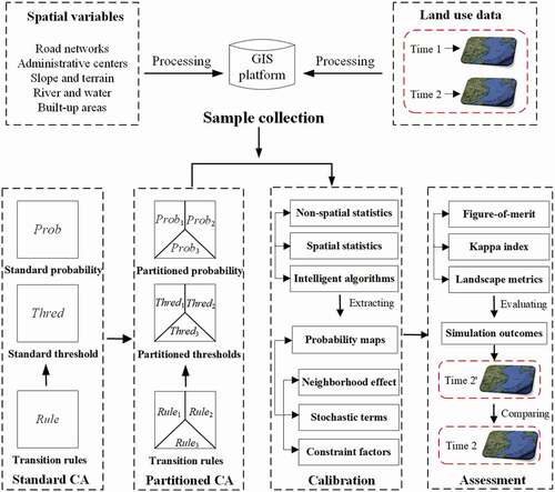
A standard CA model consists of cells and their states, cell space, neighborhood, transition rules, and time. Transition rules are the core component of a CA model, which define the future state of a cell as a uniform function of the current states of the cell and its neighborhood cells (Wu 2002). To examine the effects of partitioned transition rules upon urban growth simulation, the framework in the current work involves several parts (Figure 1). First, two relaxations were implemented to the components of standard CA transition rules for representing heterogeneous urban growth rates and laws. In particular, PDP represents separate calibrations of development probability for each partitioned zone, and PTTs indicate different criteria for selecting cells to be converted into urban cells in different zones. As the research area was divided into different zones (e.g. cities, sub-regions, or sub-areas), the dataset was split accordingly for sample collection and calibration. Then, three types of approaches, including spatial, non-spatial, and intelligent algorithms were employed to calibrate partitioned transition rules for each zone. Finally, the transition rules obtained from the training samples were applied to the entire study area, and several assessment metrics were measured to compare the performances of different models.

Figure 1. Framework of urban growth simulation in megacity regions using partitioned CA models.

2.1 Study area and zoning strategies

The Greater Wuhan Area refers to a megacity region comprising one core city of Wuhan and other eight administrative cities (i.e. Ezhou, Huanggang, Huangshi, Qianjiang, Tianmen, Xiaogan, Xianning, and Xiantao) in eastern Hubei Province in central China (Figure 2). The area covers 57,800 km² and is situated in the middle reaches of the Yangtze River. It plays an important role in economic development in Hubei Province, and is the growth pole to push forward the rise of central China. In 2007, it was approved as the national pilot area for building a resource-saving and environment-friendly society by the National Development and Reform Commission. Furthermore, massive transportation infrastructure projects, such as intercity railways and a ring expressway have been approved or under active construction during the past two decades. Therefore, the Greater Wuhan Area has experienced rapid and unparalleled urban land expansion, accompanied by numerous environmental and ecological problems. Due to its large-scale urbanization and outstanding position for regional development in China, the Greater Wuhan Area is particularly an ideal area for testing the performances of various urban CA models.

Figure 2. Urban land change in the Greater Wuhan Area during 2005–2015 (r represents the ratio of urban growth area to the urban area in 2005).

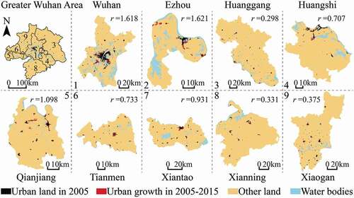
Given data availability, two land use maps covering the Greater Wuhan Area in the year of 2005 and 2015 were collected from the National Land-Use/Cover Database of China (NLUD-C). The NLUD-C was established in a project organized by the Chinese Academy of Sciences, and it has been the main source of authoritative data for studies on land use dynamics in China (Lai et al. 2016). The land use types of the NLUD-C were interpreted from satellite images using Landsat Thematic Mapper, the China–Brazil Earth Resources Satellite, and Huanjing-1A (Zhang et al. 2014). A classification system of six major land use classes was used in the NLUD-C, including cultivated land, woodland, grassland, waterbodies, built-up land, and unused land (Lai et al. 2016). The built-up land was further divided into three types, namely, urban built-up land, rural settlement, and industry–traffic land. The current work reclassified the land use data as urban built-up land, waterbodies, and other land. The NLUD-C accuracies are more than 90% according to a nationwide field verification (Zhang et al. 2014). As shown in Figure 2, urban land change in the Greater Wuhan Area during 2005 − 2015 was identified and mapped at the spatial resolution of 30 m. It was found that large amounts of urban land were concentrated in the central areas of Wuhan, and urban growth patterns in most cities were scattered.

Spatial zoning operates the partition of the study area into several homogeneous sub-regions according to specific criteria, and the transition probability for each sub-region will be calculated independently. Different zoning approaches and strategies have been used, such as division based on land use attributes, administrative division, and development planning division (Yin et al. 2018). However, division based on land use attributes may suffer from the fragmented and mixed land uses and lack of consideration of spatial administration and planning (Qian et al. 2020). Besides, development planning division has been rarely used due to the difficulty of spatial explicit assessment and interpretation of planning policies. In current study, administrative division will be employed to partition zones. Firstly, megacity regions in China are particularly large areas with very complicated and diverse geographical entities, which comprise a number of prefecture- or province-level cities and contain both actual urbanized areas and rural landscapes (Yeh and Chen 2020). It is difficult to acquire spatially regular and geographically meaningful zones using division approaches based on land use attributes or other socio-economic characteristics. Secondly, administrative boundaries play an important role in planning, management, and governance of Chinese cities (Xu and Yeh 2009; Wang and Yeh 2019). In China, local governments compete with each other, and their policies have profound effects on urban growth patterns in this area. Finally, the amount of new construction land is strictly planned and controlled through the annual land use plan made by different administrative levels of governments in China (Han and Lai 2012). This substantially contributes to various urban growth rates in different cities in China.

2.2 Proposed method

2.2.1 Standard CA framework for urban simulation

A conceptual formula of the standard CA framework for urban growth simulation can be written as follows:

(1) $S^{t+1}=f(S^t,P_0,\mathrm{\Omega },CONS,RND)$(1)

where S^t+1 denotes the future state of the cell at a discrete time point t + 1, and f is a transition function that consists of the state of the cell (S^t) at present time point t, static development probability (SDP) (P₀) determined by a series of spatial variables, the effects of the states of neighborhood cells (Ω), constraint factors (CONS) that restrict cell state transition, and a stochastic term (RND) that represents unknown perturbations.

The essence of urban growth simulation is to evaluate the development suitability of non-urban areas. The SDP of non-urban cells is influenced by a set of proximity, socio-economic, and topographical factors (Wu 2002), which can be mathematically expressed as the following equation (2)(2) $P_0=g(S^t,\{d_1,\dots ,d_i,\dots ,d_k\})$(2) :

(2) $P_0=g(S^t,\{d_1,\dots ,d_i,\dots ,d_k\})$(2)

where g is a function determined by the current states of cells and a series of spatial factors, and d_i (i = 1, 2, …, k) is a spatial factor, such as distance to road networks, administrative centers, and rivers. The acquisition and calibration of coefficients of these spatial factors can be complicated, and different approaches have been proposed to obtain more exact development probability (P₀).

An important feature of urban CA models is the consideration of local spatial interactions through neighborhood effects (Ω). The state transition of the cell at the next time point depends on its own state and the states of neighboring cells (Dahal and Chow 2015; Zhang and Wang 2021). The neighborhood effect defined using a regular n × n window can be calculated based on the ratio of the number of urban cells (c) in the neighboring cells to all neighboring cells:

(3) $\mathrm{\Omega }=c/(n\times n-1)$(3)

The CA state transition is restricted by spatial constraints, because specific urban spaces are not permitted to convert into urban land, such as ecological reserves and basic farmlands (Yeh and Li 2001). CONS is assigned a value of 0 if a cell is restricted from development; otherwise, it is assigned 1.

A stochastic term (RND) is introduced into urban CA models to add uncertainties and unknown perturbations in the urban evolution process (Wu 2002), which can be written as:

(4) $RND=1+(-ln(\gamma ){)}^{\alpha }$(4)

where γ is a random number between 0 and 1, and α is a parameter for controlling the stochastic degree.

To assess the accumulated effects of development probability, neighborhood effect, constraint factors, and stochastic term, the product of these four effects can be calculated to obtain the final probability P of the cell converting into urban land:

(5) $P=P_0\times \mathrm{\Omega }\times CONS\times RND$(5)

2.2.2 Partitioned transition rules

After calculating the final conversion probability (P) for each non-urban cell, a comparison between P and certain predefined threshold can be conducted to determine whether a non-urban cell will be converted or not (Batty 1997). The primary form of standard CA models using such rule-based structures can be explicitly expressed as follows:

IF cell {x, y} is not already developed

& IF P {x, y} is larger than some threshold value P_thred

THEN cell {x, y} is developed

where P {x, y} is the development probability for cell {x, y} in the next time point, and P_thred is the conversion threshold value, which can be determined by the number of observed or predicted converted urban cells during targeted time periods. In standard urban CA models, development probability is calibrated and obtained for the study area as a whole, and transition threshold is the same for all non-urban cells.

However, spatial heterogeneity exists in real-world urban development processes, particularly in megacity regions where a cluster of cities with different development levels and characteristics is co-located. Spatial heterogeneity can be assessed by the complexity and variability in the distribution of urban land development and in the influence intensities of spatial driving forces (Liu, Clarke, and Chen 2020). The ignorance of spatial heterogeneity in urban growth simulation can lead to unreliable predictions and results. It may be problematic to apply the same set of transition rules to the entire study area because of the varied urban development patterns and growth rates in different cities and regions (Gao et al. 2020; Liu, Clarke, and Chen 2020). Although similar driving forces of urban growth may be shared in different areas, the extent to which they affect local development differs. For example, urban expansion in areas with advantageous infrastructures can be transportation and population driven, whereas it may be significantly blocked by topographical conditions in some remote mountain areas. Furthermore, urban land sprawls quickly in areas with booming economy and population or development priority, while it changes at a relatively slow rate in well-developed or restricted areas. The spatial differentiation in the distribution and driving forces of urban development can be represented by introducing partitioned transition rules into urban CA models (Ke, Qi, and Zeng 2016; Kazemzadeh-Zow et al. 2017; Yin et al. 2018). In particular, PDP can be used to represent various urban development patterns in partitioned zones, and PTTs can be applied to control different urban growth rates.

PDP means that different sub-regions have heterogeneous development probability. The SDP (P₀) will be calibrated and calculated for each sub-region (Ke, Qi, and Zeng 2016), which can be expressed as follows:

(6) $P_0=\{P_0^1,P_0^2,\dots ,P_0^j,\dots ,P_0^m\}$(6)

(7) $P_0^j=g(S_j^t,\{d_1^j,\dots ,d_i^j,\dots ,d_k^j\})$(7)

where$P_0^j$is the conversion probability for non-urban cells in the sub-region j (j = 1, 2, …, m),$S_j^t$is the current state of cell in the sub-region j, and$d_i^j$represents a spatial variable i in the sub-region j. The accumulated probability P in Eq. (5)(5) $P=P_0\times \mathrm{\Omega }\times CONS\times RND$(5) for the cell in sub-region j to be converted into urban land can be modified as follows:

(8) $P_j=P_0^j\times {\mathrm{\Omega }}_j\times CON{S}_j\times RN{D}_j$(8)

PTTs mean that different sub-regions have different transition thresholds. The transition threshold P_thred will be designed and obtained for each sub-region according to the number of observed or predicted developed cells and iteration times (Xia et al. 2019a). Therefore, the comparison of the accumulated development probability P and PTTs in different partitioned zones determines the future states of non-urban cells in the next time point, which can be written as follows:

(9) $S_j^{t+1}=\left\{\begin{array}{c}1\\ 0\end{array}\right.\begin{array}{cc}\hspace{0.17em}& \begin{array}{c}{P}_j\ge P_{thred}^j\\ P_j<P_{thred}^j\end{array}\end{array}$(9)

where $S_j^{t+1}$denotes the future state of the cell in sub-region j at time point t + 1.$P_{thred}^j$denotes the transition threshold value in sub-region j, which will be combined with iteration times to control total number of newly urbanized cells in sub-region j.

2.3 Model calibration using different approaches

In this study, three different types of widespread approaches were used to calibrate urban CA models, including non-spatial, spatial, and intelligent algorithms. The selection and comparison of different algorithms were used to provide a sensitivity analysis of the effects of partitioned transition rules on urban simulation. In particular, LR, which has been the most commonly applied non-spatial method, was used as the baseline for comparison. GWR, as a typical spatial regression method, was used because spatial heterogeneity of the driving forces may still exist after area partitioning. Two intelligent algorithms, including PSO and SVM, were selected as the representatives of metaheuristics and non-parametric machine learning techniques. Finally, four urban CA models, namely, LR-CA, GWR-CA, PSO-CA, and SVM-CA models were constructed.

2.3.1 The LR-CA model

LR has been widely used to associate urban development with socio-economic and spatial driving forces and to generate the potential development probability map. The state of a cell in urban CA modeling is dichotomous and can be represented by a dummy variable, where the values of 1 and 0 indicate the presence and absence of urban growth. The logit curve or logit function is popularly used to estimate the probability of a cell to be developed (Wu 2002). This basic and scalable form is improved and expanded in many other urban CA models. In LR-CA models, the SDP of non-urban cells can be expressed as follows:

(10) $P_0^j=exp(a_0^j+\sum _{i=1}^k{a}_i^j\times d_i^j)/(1+exp(a_0^j+\sum _{i=1}^k{a}_i^j\times d_i^j))$(10)

where $P_0^j$denotes the SDP for non-urban cells in the sub-region j (j = 1, 2, …, m), $d_i^j$denotes a spatial variable i in the sub-region j,$a_0^j$is a constant, and$a_i^j$denotes the local coefficient of the spatial variable i in the sub-region j.

2.3.2 The GWR-CA model

GWR is a set of spatial regression techniques that allow local rather than global coefficients to be estimated (Fotheringham, Brunsdon, and Charlton 2003). GWR is capable of identifying spatially varying relationships between urban development and various driving factors (Mirbagheri and Alimohammadi 2017). Based on GWR, the SDP in the equation (10)(10) $P_0^j=exp(a_0^j+\sum _{i=1}^k{a}_i^j\times d_i^j)/(1+exp(a_0^j+\sum _{i=1}^k{a}_i^j\times d_i^j))$(10) can be amended as follows:

(11) $P_0^j(u,v)=\frac{exp(a_0^j(u,v)+\sum _{i=1}^k{a}_i^j(u,v)\times d_i^j(u,v)+\epsilon (u,v))}{(1+exp(a_0^j(u,v)+\sum _{i=1}^k{a}_i^j(u,v)\times d_i^j(u,v)+\epsilon (u,v)))}$(11)

where (u, v) denotes the coordinates of a cell in space, and ε denotes an error term. It is noted that equation (10)(10) $P_0^j=exp(a_0^j+\sum _{i=1}^k{a}_i^j\times d_i^j)/(1+exp(a_0^j+\sum _{i=1}^k{a}_i^j\times d_i^j))$(10) is a special case of equation (11)(11) $P_0^j(u,v)=\frac{exp(a_0^j(u,v)+\sum _{i=1}^k{a}_i^j(u,v)\times d_i^j(u,v)+\epsilon (u,v))}{(1+exp(a_0^j(u,v)+\sum _{i=1}^k{a}_i^j(u,v)\times d_i^j(u,v)+\epsilon (u,v)))}$(11) in which the local coefficient of each spatial variable is assumed to be a constant within each sub-region. The samples near to a cell have greater influences in parameter estimation of this cell than those located farther away. Various weighting schemes have been proposed to represent such varying influences based on the proximity of a sample x to its surrounding sample y, among which the distance decay function is widely used (Feng, Liu, and Tong 2018; Gao et al. 2020) and defined as follows:

(12) $w_{xy}=exp(-\frac{d_{xy}^2}{{\beta }^2})$(12)

where w_xy denotes the spatial weight of the impacts between the two samples, d_xy denotes the distance, and β refers to the bandwidth.

2.3.3 The PSO-CA and SVM-CA models

In the current work, two intelligent algorithms were employed, including PSO and SVM. PSO is a metaheuristic method that optimizes a problem by simulating the movement of organisms in bird flocks (Poli, Kennedy, and Blackwell 2007). The calibration of urban CA models using PSO is essentially a process of minimizing the residuals of urban simulation, thus retrieving better coefficients of driving factors and producing more accurate simulation outcomes. The sum of squared errors of prediction (SSE) is the objective function for guiding the optimization process in the PSO-CA model (Feng, Liu, and Tong 2018), which can be calculated by comparing the simulated and actual results for all samples as follows:

(13) $F_j(d_1^j,\dots ,d_i^j,..,d_k^j)=\sum _{l=1}^s(P_0^j(l)-S^t(l){)}^2$(13)

where F_j is the objective function, s is the number of samples for calibrating transition rules in the sub-region j,$P_0^j(l)$denotes the SDP of sample cell l (l = 1, 2, …, s) calculated by spatial variables, which is equal to equation (10)(10) $P_0^j=exp(a_0^j+\sum _{i=1}^k{a}_i^j\times d_i^j)/(1+exp(a_0^j+\sum _{i=1}^k{a}_i^j\times d_i^j))$(10) , and$S^t(l)$denotes the actual state of sample cell l, with value 1 representing that cell l changes to urban land, and 0 representing that cell l remains as non-urban land. Suppose that k spatial variables are selected in an urban CA model and a number of feasible solutions for the coefficients are initialized, which can be projected as a (k + 1)-dimensional search space and particle populations in PSO. Each particle has a position in the search space, a velocity for the particle’s movement, and an evaluation value based on the objective function (Poli, Kennedy, and Blackwell 2007). The movement of each particle is influenced by the current local best position acquired by the particle, as well as the current global best position acquired by all particles (Poli, Kennedy, and Blackwell 2007). The position and velocity of particles are thus updated during the process of optimization, which are expected to move the populations toward the best positions in the search space.

SVM is a supervised nonparametric learning approach whose performance has been proven in previous studies of urban CA modeling (Yang, Li, and Shi 2008; Karimi et al. 2019). SVM maps the training dataset to points in the Hilbert space where an optimal hyperplane separates training examples into two categories. An optimal separating hyperplane is equally distant from the closest data points from both categories, and those points with the minimum distance to the hyperplane are called support vectors. The margin is the distance between the separating hyperplane and its support vectors. By maximizing the margin between the two categories of training data, SVM finds the optimal separating hyperplane that minimizes the measure of empirical error (Karimi et al. 2019). This margin maximization capability provides SVM with a good generalization performance independent of data distribution. The trained SVM model are then used to map the input dataset into the same space and assign new examples to a category based on their locations. In SVM, the choice of kernel is important for the performance of a constructed machine, which defines the functional form of all possible solutions. In the current work, the radial basis function (RBF) kernel was used according to the research by Karimi et al. (2019).

2.4 Assessment methods

For assessing the simulation outcomes and comparing the performances of different models, three types of indices were implemented according to the review by Tong and Feng (2020), including Kappa coefficient, figure of merit (FoM), and landscape metrics. The Kappa coefficient has been widely used to evaluate the overall agreement of quantity and location between the simulation and reference maps. A pixel-by-pixel comparison was conducted to produce a confusion matrix for the calculation of Kappa coefficient (Pontius and Millones 2011). To assess the overlapping between the observed and simulated converted areas, the FoM metric was also applied in the current study. FoM is defined as the ratio of the intersection of observed converted areas and simulated converted areas to the union of observed converted areas and simulated converted areas (Pontius et al. 2008). FoM ranges from 0%, meaning no overlapping, to 100%, meaning perfect overlapping. It can be expressed as follows:

(14) $FoM=\frac{\mathrm{H}\mathrm{i}\mathrm{t}\mathrm{s}}{\mathrm{M}\mathrm{i}\mathrm{s}\mathrm{s}\mathrm{e}\mathrm{s}+\mathrm{H}\mathrm{i}\mathrm{t}\mathrm{s}+\mathrm{F}\mathrm{a}\mathrm{l}\mathrm{s}{\mathrm{e}}^{\hspace{0.17em}}\mathrm{A}\mathrm{l}\mathrm{a}\mathrm{r}\mathrm{m}\mathrm{s}}$(14)

where Misses are the area of errors observed as urban growth but simulated as persisted non-urban cells, Hits are the area of correctness observed and simulated as urban growth, and False Alarms are the area of errors observed as persisted non-urban cells but simulated as urban growth.

Spatial patterns of observed and simulated urban growth reveal important aspects of similarities, which cannot be reflected in the quantity agreement and location agreement (Wang et al. 2020; Zhang et al. 2020). Therefore, besides Kappa and FoM, landscape metrics were adopted to assess simulation outcomes. Two landscape metrics are selected, including the mean area of patches (Area_MN) and landscape shape index (LSI). Area_MN represents the degree of landscape fragmentation. LSI represents the complexity degree of landscape shapes, which is calculated as the normalized ratio of total length of edge to total area. In this study, these assessment methods were conducted for the whole region and sub-regions to evaluate the performance of different models. To characterize different urban development patterns in sub-regions, the landscape expansion index (LEI) was measured to divide urban growth into outlying, edge-expansion, and infilling types, and its calculation was based on the approach proposed by Liu et al. (2010).

3 Implementation and results

3.1 Spatial variables

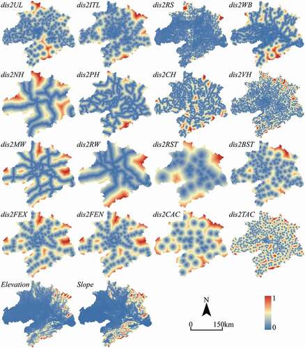
Taking previous urban simulation studies into account (Seto, Güneralp, and Hutyra 2012), four major groups of driving forces were selected to explain urban growth in the Greater Wuhan Area, including proximity to existing built-up land, proximity to transportation lines, proximity to public infrastructures, and topographical and geographical conditions. As shown in Table 1, three spatial factors indicating the proximity to existing built-up land were derived from the land use data, six spatial factors indicating the proximity to transportation lines were derived from road network data, six spatial factors indicating the proximity to public infrastructures were derived from point of interests (POI) data, and three spatial variables indicating topographical and geographical conditions were derived from terrain and land use data. The main data sources in this study can be downloaded from Open Street Map (https://www.openstreetmap.org), Baidu Map (https://map.baidu.com), Geospatial Data Cloud (http://www.gscloud.cn), and Resource and Environment Data Cloud Platform (http://www.resdc.cn). As the data sets are large, a stratified random sampling strategy was used to collect the training data of a reasonable size (Feng, Liu, and Tong 2018). 8,000 sample cells were collected in total from land use and spatial variable maps, including 4,000 sample cells of urban gain and 4,000 sample cells of non-urban persistence. To guarantee the comparability of transition rules with and without area partitioning, these samples were selected from different sub-regions based on their area proportions (Table 2).

Table 1. List of spatial variables related to urban expansion in the Greater Wuhan Area.

Categories	File type	Unit	Codes	The meaning of spatial variables	Source
Proximity to existing built-up land	GRID	meter	dis2UL	Distance to urban settlement	www.resdc.cn
	GRID	meter	dis2ITL	Distance to industry-traffic land
	GRID	meter	dis2RS	Distance to rural settlement
Proximity to transportation lines	Shapefile	meter	dis2NH	Distance to national roads	openstreetmap.org
	Shapefile	meter	dis2PH	Distance to provincial roads
	Shapefile	meter	dis2CH	Distance to county roads
	Shapefile	meter	dis2VH	Distance to village roads
	Shapefile	meter	dis2MW	Distance to motorway
	Shapefile	meter	dis2RW	Distance to railway
Proximity to public infrastructures	Shapefile	meter	dis2FEX	Distance to freeway exit	map.baidu.com
	Shapefile	meter	dis2FEN	Distance to freeway entrance
	Shapefile	meter	dis2RST	Distance to railway station
	Shapefile	meter	dis2BST	Distance to bus station
	Shapefile	meter	dis2CAC	Distance to county administrative center
	Shapefile	meter	dis2TAC	Distance to township administrative center
Topographical and geographical conditions	GRID	meter	dis2WB	Distance to water bodies	LINKwww.resdc.cn
	GRID	meter	Elevation	The elevation above sea level	www.gscloud.cn
	GRID	degree	Slope	Slope of the ground

Table 2. The number of samples in the study area and its sub-regions.

Areas	Area Proportion (%)	Samples	Urban Samples	Non-urban Samples
Greater Wuhan Area	100	8,000	4,000	4,000
Wuhan	14.7	1,176	588	588
Ezhou	2.8	226	113	113
Huanggang	30	2,400	1,200	1,200
Huangshi	7.9	628	314	314
Qianjiang	3.5	280	140	140
Tianmen	4.6	366	183	183
Xiaogan	15.3	1,228	614	614
Xianning	16.8	1,346	673	673
Xiantao	4.4	350	175	175

As shown in Figure 3, all data were normalized into the range of 0 to 1 and resampled to the same spatial resolution (30 m) with land use maps. Urban development can be influenced by existing built-up land, and many new towns and counties have emerged near to other human settlements, leading to the consolidation of urban areas. Thus, the proximity to existing built-up land was selected as an important driving force, including distance to urban settlement, distance to rural settlement, and distance to industry-traffic land. Transportation lines can facilitate population and material movements within and between urban areas, which were identified and classified as national, provincial, county, and village roads, motorway, and railway in this study. The distances to these transportation lines were taken as main determinants of urbanization. Public infrastructure plays a vital role in land investments and location choices, as areas closer to different facilities are more likely to be developed. Thus, the accessibility to freeway entrances and exits, railway stations, bus stations, county centers, and town centers were chosen. Furthermore, factors related to topographical and geographical conditions, such as elevation, slope, and water bodies, may restrict and block continuous urban land expansion.

Figure 3. Visualization of spatial variables (see Table 1 for the meanings of the codes and variables).

3.2 Model calibration and transition potentials

As shown in Table 3 and Figure 4, Figure 5, Figure 6 coefficient estimation using different approaches is generally consistent in sign, but substantially differs in the absolute values. Furthermore, there are great variations between coefficients obtained from different sub-regions, which represent the significantly varied effects of spatial variables on urban land use change in different areas. The results with and without area partitioning are particularly different, indicating the necessity of constructing partitioned transition rules. For GWR parameters, each factor has both positive and negative coefficients, indicating that its effect on urban growth can be opposite in different areas. Besides, the continuous surface of GWR parameters was interrupted after area partitioning. Due to stochastic optimization involved in PSO, different solutions can be found for the same samples. To address such uncertainties, the PSO algorithm was run ten times for each sample input, and the result with the best objective function value was applied to calibrate the CA transition rules. Figure 7 shows the convergence curves of PSO algorithm for the study area and its sub-regions, which are relatively stable and yield the finest objective function value at the early and middle stages of optimization process.

Figure 4. Coefficient estimates of urban CA transition rules for the entire area and separate sub-regions using PSO.

Figure 5. Coefficient estimates of urban CA transition rules for the entire area using GWR.

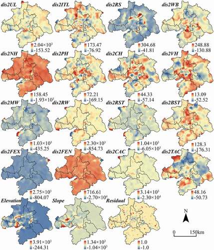
Figure 6. Coefficient estimates of urban CA transition rules for nine separate sub-regions using GWR.

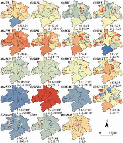
Figure 7. The convergence curves of PSO algorithm for the entire area and separate sub-regions.

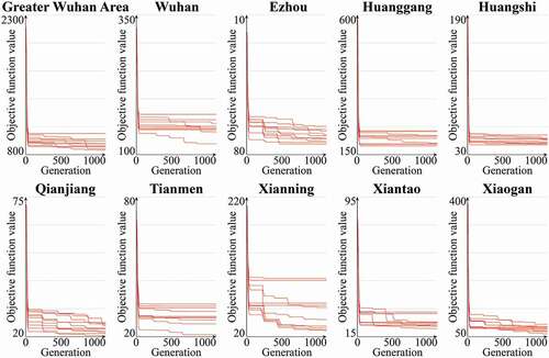
Table 3. Coefficient estimates of urban CA transition rules for the entire area and separate sub-regions using LR.

Variables	Greater Wuhan Area	Wuhan	Ezhou	Huanggang	Huangshi	Qianjiang	Tianmen	Xiantao	Xianning	Xiaogan
dis2UL	−19.692	−12.024	6.169	−8.313	−16.563	−17.221	−70.746	−24.062	−62.892	−38.085
dis2ITL	−2.271	−9.749	−52.561	−2.143	−1.535	−2.207	−9.044	−8.397	−4.171	−5.563
dis2RSP	−.166	−.615	−10.120	12.024	1.631	−2.698	−23.730	6.975	−5.714	2.551
dis2WB	−1.480	−1.220	13.033	−2.032	−6.440	−5.513	10.580	−8.851	1.713	−2.594
dis2NH	.776	−1.070	−32.007	1.571	−5.590	−19.267	−5.561	−20.774	.003	−.245
dis2PH	−9.663	−1.433	−21.862	−8.645	−4.359	4.505	−20.076	−5.206	2.390	−9.311
dis2CH	−2.390	.414	−12.098	−4.723	1.593	−1.857	−23.140	−8.292	2.536	.911
dis2VH	−19.090	−13.180	−7.028	−11.658	−20.628	−6.499	4.158	−26.614	−29.049	−32.878
dis2MW	−3.486	.994	87.221	−5.184	−6.315	32.330	3.312	−13.517	1.574	1.806
dis2RW	.517	−3.950	26.790	1.230	−2.026	36.298	−2.524	44.567	−5.873	.517
dis2RST	−2.092	−.243	−34.402	3.058	−3.871	19.677	−2.461	−11.739	2.128	−7.901
dis2BST	.388	.685	−2.656	1.758	−12.295	−9.360	−23.138	5.033	−3.900	−9.591
dis2FEX	27.430	29.174	102.983	13.774	72.951	−167.018	193.329	−88.639	17.014	−30.321
dis2FEN	−27.260	−29.249	−227.732	−13.018	−74.417	88.261	−200.840	94.853	−19.252	33.222
dis2CAC	2.264	5.061	1.499	1.953	19.698	−13.476	24.067	−9.138	1.430	3.549
dis2TAC	−2.924	−3.043	−32.791	−3.453	−15.261	−13.003	1.206	−8.399	−7.811	−5.369
Elevation	10.978	−5.131	74.356	−7.247	11.774	7.555	−12.727	10.522	4.527	46.132
Slope	−4.228	1.832	−41.788	−10.921	−3.195	−9.336	−3.552	−4.009	4.809	−91.261
Constant	4.183	3.283	47.126	4.213	9.758	18.066	22.733	10.542	6.695	9.076

The SDP maps were obtained based on the above six sets of CA coefficients acquired by different approaches and zoning schemes. The trained SVM models based on different samples were used to calculate the SDP maps for the study area and its sub-regions. As shown in Figure 8, differences can be observed between SDP maps based on LR, GWR, PSO, and SVM, as well as between results with and without area partitioning. The distribution of areas with relatively high conversion potentials is more scattered in maps using LR than in those using GWR, PSO, and SVM. Furthermore, the areas with high conversion potentials are larger in maps using LR and PSO or without area partitioning than in these using GWR and SVM or with area partitioning. Therefore, the simulation results based on the eight types of models may be greatly different because their differences in development probability are substantial. In addition to calibrating CA coefficients, the set of transition thresholds is another key step for constructing urban CA models, which was defined based on the total amount of available land for development during the calibration time interval (Xia et al. 2019a). For comparison, the eight urban CA models based on the above SDP maps adopted two types of thresholds, including standard transition threshold designed for the whole region and PTTs designed for each sub-region. Finally, 16 urban CA models were constructed and applied to simulate urban growth in the Greater Wuhan Area during 2005 − 2015.

Figure 8. Comparison of static development probability maps based on different approaches and zoning schemes.

3.3 Results and model comparison

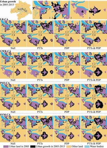
In this section, the simulation accuracies of standard urban CA models and partitioned urban CA models were compared to preliminarily examine the effects of PDP and PTTs. Particularly, four types of model structure were involved, including the urban CA models without considering PDP and PTTs, the urban CA models considering PDP, the urban CA models considering PTTs, and the urban CA models considering PDP and PTTs. In addition, four approaches were used in the calibration process of urban CA models, including LR, GWR, PSO, and SVM. Therefore, there were sixteen different urban CA models. To reduce the influence of uncertainties and unknown perturbations caused by the stochastic term, each urban CA model was run ten times and the mean accuracies of 10 simulation results were used in the current study. The entire study area and four local positions experiencing dramatic changes were selected to visualize the simulation results of different urban CA models, as well as their spatial differences. Figure 9 shows the simulated distribution of urban growth in the Greater Wuhan Area during 2005 − 2015, and the results of different urban CA models with and without considering PDP and PTTs are significantly different. To conduct more intuitive and meaningful comparisons, some quantitative metrics were measured and used to evaluate the differences between simulation results.

Figure 9. Simulation results of different urban CA models with and without considering partitioned transition rules.

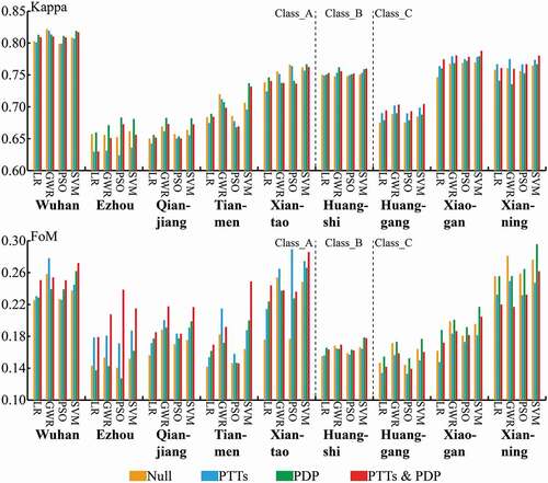
Table 4 presents the Kappa coefficients and FoM values of the simulation outcomes of different urban CA models, and Figure 10 shows the ratio of Area_MN or LSI based on simulation maps to that based on reference maps. Due to the consideration of spatial non-stationarity, GWR-CA models can produce much more accurate simulation results than LR-CA, PSO-CA, and SVM-CA models, as the values of Kappa and FoM are larger and Area_MN and LSI are closer to reality. LR-CA models have the poorest performance according to the overall accuracies of the study area, while the improvements of PSO-CA models are small. It is noted that Area_MN of simulated results is much smaller than reality, which is due to the huge number of simulated urban patches. More importantly, it was found that the overall simulation accuracies of all four CA-based models using PPTs were improved compared to the traditional CA models, and LR-CA, PSO-CA, and SVM-CA models using PDP are much better than these without considering PDP. Furthermore, the performance of LR-CA, PSO-CA, and SVM-CA models can be significantly improved through the combination of PDP and PTTs. GWR-CA models are negatively impacted by PDP, which may be partly due to that area partitioning obstructs the local interactions of spatial variables across boundaries. However, the evaluation of simulation outcomes for the entire region cannot provide answers and more information. Besides, as the Greater Wuhan Area comprises a cluster of administrative cities covering vast built-up and non-built-up territory, it might be meaningful and comparable to assess the simulation accuracies for each sub-region. Furthermore, the effects of PDP and PTTs on urban simulation may greatly vary in sub-regions.

Figure 10. Spatial similarities between the simulation results of different urban CA models and the actual data (y-axis represents the ratio of simulated landscape metrics to observed landscape metrics).

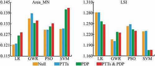
Table 4. The overall simulation accuracies of different urban CA models in the Greater Wuhan Area.

CA Models	Kappa	Improvement (%)	FoM	Improvement (%)
LR-CANull	0.7561	–	0.1872	–
LR-CAPTTs	0.7573	0.12	0.1898	0.26
LR-CAPDP	0.7610	0.49	0.1976	1.04
LR-CAPTTs & PDP	0.7636	0.75	0.2032	1.60
GWR-CANull	0.7703	–	0.2178	–
GWR-CAPTTs	0.7725	0.22	0.2229	0.51
GWR-CAPDP	0.7663	−0.40	0.2091	−0.87
GWR-CAPTTs & PDP	0.7683	−0.20	0.2135	−0.43
PSO-CANull	0.7582	–	0.1916	–
PSO-CAPTTs	0.7598	0.16	0.1951	0.35
PSO-CAPDP	0.7627	0.45	0.2012	0.96
PSO-CAPTTs & PDP	0.7652	0.70	0.2067	1.51
SVM-CANull	0.7654	–	0.2072	–
SVM-CAPTTs	0.7664	0.10	0.2093	0.21
SVM-CAPDP	0.7746	0.92	0.2275	2.03
SVM-CAPTTs & PDP	0.7766	1.12	0.2320	2.48

4 Discussion

The evaluation of different models’ performances was conducted for all the sub-regions. As shown in Figure 11, the simulation accuracies of LR-CA, PSO-CA, and SVM-CA models were significantly improved after considering PDP in most of sub-regions. In contrast, PDP performed poorly for GWR-CA models with decreased simulation accuracies in most of sub-regions. In particular, PDP has great positive effects on the simulation outcomes of LR-CA models in all sub-regions except for Xianning, on those of PSO-CA models in Wuhan, Ezhou, Huanggang, Huangshi, and Xiaogan, and on those of SVM-CA models in all sub-regions. The performances of LR-CA models in Xianning, GWR-CA models in Wuhan, Tianmen, Xiantao, and Xianning, and PSO-CA models in Tianmen and Xiantao, were dramatically decreased after adopting PDP. In comparison, the results of PTTs showed consistent and regular patterns in the sub-regions. As shown in Figure 11, three types of sub-regions were found based on their improvements in terms of Kappa coefficient and FoM. PTTs significantly improved the Kappa coefficients of all four CA-based models in Class_C regions but with FoM values decreased, whereas PTTs significantly improved FoM values of all four CA-based models in Class_A regions but with Kappa coefficients decreased in these sub-regions. Furthermore, the combination of PDP and PTTs can produce the most accurate simulations for the four CA-based models in many sub-regions.

Figure 11. The simulation accuracies of different urban CA models in the sub-regions.

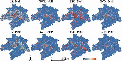
To further explore the underlying reasons, the effects of PDP on SDP of available cells (Figure 12a as null model and 12b as adopting PDP) and observed converted cells (Figure 12c as null model and 12d as adopting PDP) were analyzed. It can be found that PDP can significantly improve the SDP of available cells for the methods of LR, PSO, and SVM, represented by a more concentrated distribution of SDP for available cells and the increasing proportions of SDP equal to the actual values (i.e. 1) for observed converted cells. However, PDP may not be applicable for GWR because SDP obtained by spatially heterogeneous methods is good and not further improved by PDP. Besides, SDP in Wuhan and Huanggang was less improved by PDP according to their curves, which may be due to the relatively small proportions of edge-expansion growth (see Figure 13). According to the existing literature, urban CA models have limitations in the simulation of isolated urban development (Liu et al. 2014). As SDP in different sub-regions was dramatically changed, the number of converted cells based on different urban CA models was calculated to reflect how the simulated growth rates were subsequently influenced (Table 5). The root mean squared error (RMSE) and standard deviation (SD) of simulated growth rates were analyzed. It can be found that the difference of simulated growth rates between sub-regions becomes smaller and the difference between the actual and simulated development is larger after adopting PDP, represented by the decreased SD and increased RMSE. This may help to understand the poor performance of PDP on GWR-CA model, as the SDP maps obtained by GWR were less improved and the simulated growth rates based on GWR-CA models were negatively influenced by PDP. Besides, the sub-regions experiencing large growth rates were often underestimated in null models, and PDP may exacerbate such underestimation. This may be the reason why the improvements brought by PDP were complicated in different sub-regions.

Figure 12. The distribution of static development probability of available cells and observed converted cells (x-axis refers to the probability range, and y-axis refers to the percentage of cells with a certain probability).

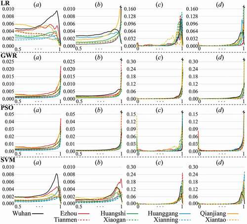
Figure 13. The comparison of different urban growth patterns in sub-regions using LEI.

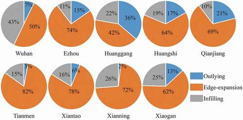
Table 5. Observed and simulated growth rates (converted cells/total urban cells) based on different urban CA models.

Sub-regions	Reference	LR-CA		GWR-CA		PSO-CA		SVM-CA		PTTs
		Null	PDP	Null	PDP	Null	PDP	Null	PDP
Wuhan	1.618	1.523	1.313	1.356	1.394	1.638	1.449	1.501	1.466	1.618
Ezhou	1.621	0.819	0.735	0.924	0.638	0.854	0.393	0.834	0.675	1.621
Huanggang	0.298	0.395	0.398	0.399	0.397	0.388	0.394	0.397	0.416	0.298
Huangshi	0.707	0.695	0.736	0.776	0.631	0.728	0.723	0.739	0.720	0.707
Qianjiang	1.098	0.870	0.971	0.898	0.755	0.896	1.003	0.862	0.821	1.098
Tianmen	0.733	0.600	0.656	0.510	0.560	0.609	0.748	0.533	0.452	0.733
Xiaogan	0.375	0.512	0.502	0.488	0.485	0.429	0.437	0.463	0.461	0.375
Xianning	0.331	0.433	0.536	0.494	0.571	0.455	0.493	0.456	0.503	0.331
Xiantao	0.931	0.565	0.736	0.812	0.921	0.323	0.824	0.701	0.747	0.931
RMSE	–	0.315	0.335	0.281	0.372	0.340	0.421	0.301	0.359	0.000
SD	0.481	0.324	0.259	0.287	0.282	0.384	0.328	0.320	0.306	0.481

PTTs can correct the underestimated or overestimated number of cells to be converted in sub-regions (Table 5). It is found that the number of simulated converted cells in Huanggang, Xiaogan, and Xianning was greatly overestimated when PTTs were not considered in urban CA models. Comparatively, the number of simulated converted cells was largely underestimated in Ezhou and Xiantao, where PTTs performed particularly well. As large amounts of cells of non-urban persistence are ignored in the definition of FoM, the increase of simulated developed areas could expand the overlapping between simulated and observed changes (Hits) and result in improved FoM values (see Table 6). However, the increased number of simulated growth cells may not yield better results in terms of Kappa coefficients when SDP is of low levels of accuracy. For example, the SDP obtained by PSO method performed poorly in Xiantao represented by the relatively large proportions of SDP equal to zero for observed converted cells (Figure 12c), and PTTs dramatically improved the FoM values of PSO-CA models in Xiantao but with the Kappa coefficients slightly decreased.

Table 6. The number of Misses, Hits, False Alarms, and simulated growth cells for simulation results based on different urban CA models.

Class	City	Index	LR-CA				GWR-CA				PSO-CA				SVM-CA
			Null	PTTs	PDP	PDP&PTTs	Null	PTTs	PDP	PDP&PTTs	Null	PTTs	PDP	PDP&PTTs	Null	PTTs	PDP	PDP&PTTs
A	Wuhan	Misses	108,457	105,727	111,479	101,555	105,077	96,086	107,996	100,854	106,125	106,680	107,021	101,599	106,359	102,716	102,259	97,247
		Hits	56,882	59,612	53,860	63,784	60,262	69,253	57,343	64,485	59,214	58,659	58,318	63,740	58,980	62,624	63,080	68,092
		False Alarms	87,090	93,356	70,234	89,184	67,941	83,715	74,391	88,483	95,613	94,309	78,622	89,228	82,918	90,345	75,497	84,876
		Simulated growth	143,972	152,968	124,094	152,968	128,203	152,968	131,734	152,968	154,827	152,968	136,940	152,968	141,898	152,968	138,577	152,968
	Ezhou	Misses	24,313	20,931	24,695	20,912	23,711	20,837	24,736	19,727	24,319	21,253	25,734	18,501	23,973	20,569	24,048	19,423
		Hits	5603	8985	5221	9004	6205	9079	5180	10,189	5597	8664	4182	11,415	5943	9347	5869	10,493
		False Alarms	9238	20,382	8090	20,363	10,534	20,288	6388	19,178	9884	20,704	2931	17,952	9176	20,020	6355	18,874
		Simulated growth	14,840	29,367	13,312	29,367	16,739	29,367	11,569	29,367	15,481	29,367	7113	29,367	15,119	29,367	12,224	29,367
	Qianjiang	Misses	20,603	19,325	19,543	18,815	19,410	18,263	19,833	17,652	20,042	18,885	19,418	18,883	19,974	18,603	19,345	17,688
		Hits	6270	7548	7330	8059	7464	8610	7040	9221	6831	7988	7455	7990	6899	8270	7528	9185
		False Alarms	13,299	17,150	14,504	16,640	12,743	16,088	9941	15,477	13,322	16,710	15,111	16,708	12,491	16,428	10,947	15,513
		Simulated growth	19,569	24,698	21,834	24,698	20,207	24,698	16,980	24,698	20,153	24,698	22,566	24,698	19,390	24,698	18,475	24,698
	Tianmen	Misses	17,337	16,452	16,511	15,947	16,545	14,549	16,611	15,242	17,164	16,309	16,629	16,711	16,946	15,370	16,366	13,561
		Hits	4955	5841	5781	6345	5747	7744	5681	7050	5128	5983	5663	5581	5346	6922	5926	8731
		False Alarms	12,637	15,660	13,452	15,155	9212	13,757	10,741	14,450	12,725	15,517	16,287	15,919	10,296	14,578	7341	12,769
		Simulated growth	17,592	21,500	19,233	21,500	14,959	21,500	16,422	21,500	17,853	21,500	21,949	21,500	15,643	21,500	13,267	21,500
	Xiantao	Misses	20,519	17,554	18,222	16,514	16,843	15,816	16,800	16,731	21,515	15,018	17,640	16,782	17,467	15,492	16,857	15,122
		Hits	6402	9367	8700	10,407	10,078	11,105	10,121	10,190	5406	11,903	9281	10,139	9274	11,429	10,064	11,799
		False Alarms	9470	16,773	11,965	15,733	12,725	15,035	15,729	15,950	3669	14,237	13,848	16,001	10,409	14,711	10,903	14,341
		Simulated growth	15,872	26,140	20,664	26,140	22,804	26,140	25,850	26,140	9075	26,140	23,129	26,140	19,684	26,140	20,967	26,140
B	Huangshi	Misses	26,874	26,729	26,018	26,333	25,591	26,282	26,850	26,022	26,439	26,686	26,246	26,396	25,964	26,290	25,441	25,588
		Hits	9615	9760	10,471	10,156	10,898	10,207	9639	10,467	10,050	9803	10,244	10,093	10,526	10,199	11,048	10,901
		False Alarms	25,491	25,981	26,721	25,585	28,310	25,534	22,250	25,274	26,771	25,938	26,276	25,648	26,852	25,542	25,332	24,840
		Simulated growth	35,105	35,741	37,192	35,741	39,208	35,741	31,889	35,741	36,822	35,741	36,520	35,741	37,378	35,741	36,380	35,741
C	Huanggang	Misses	53,113	56,779	52,158	55,998	50,248	54,552	50,143	54,343	53,545	56,871	52,502	56,245	51,139	55,213	49,106	54,177
		Hits	19,004	15,338	19,959	16,119	21,869	17,565	21,974	17,774	18,572	15,246	19,615	15,872	20,979	16,904	23,011	17,940
		False Alarms	57,546	42,378	57,087	41,597	55,307	40,151	54,826	39,942	56,504	42,470	56,620	41,844	55,830	40,812	58,070	39,776
		Simulated growth	76,550	57,716	77,046	57,716	77,176	57,716	76,800	57,716	75,077	57,716	76,234	57,716	76,808	57,716	81,081	57,716
	Xiaogan	Misses	29,248	31,974	27,658	30,537	27,172	29,900	27,111	29,708	29,220	30,493	28,468	29,996	27,815	30,004	26,519	28,716
		Hits	12,914	10,187	14,503	11,624	14,989	12,261	15,050	12,453	12,941	11,668	13,693	12,165	14,346	12,157	15,642	13,445
		False Alarms	37,591	26,789	34,976	25,352	33,149	24,715	32,786	24,523	29,369	25,308	29,374	24,811	31,312	24,819	29,884	23,531
		Simulated growth	50,504	36,976	49,478	36,976	48,138	36,976	47,836	36,976	42,310	36,976	43,067	36,976	45,658	36,976	45,526	36,976
	Xianning	Misses	20,745	24,092	18,460	24,707	17,949	23,276	17,686	24,851	20,071	24,125	18,902	24,097	19,104	23,384	16,920	22,697
		Hits	17,259	13,911	19,543	13,296	20,054	14,727	20,317	13,152	17,932	13,878	19,101	13,906	18,899	14,619	21,083	15,307
		False Alarms	29,605	21,851	38,473	22,466	33,379	21,035	41,472	22,610	31,338	21,884	34,250	21,856	30,393	21,143	33,289	20,456
		Simulated growth	46,864	35,762	58,016	35,762	53,434	35,762	61,788	35,762	49,270	35,762	53,351	35,762	49,292	35,762	54,371	35,762

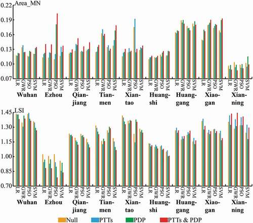
The Area_MN and LSI values provide the similarity of landscape patterns between simulation results and observed urban maps. As shown in Figure 14, PTTs can significantly increase the mean size of urban patches for simulation outcomes in Ezhou, Huangshi, Qianjiang, Tianmen, and Xiantao. It is found that PTTs greatly reduced the number of newly developed cells and increased the degree of landscape fragmentation in Huanggang and Xianning, as opposite to that in most other sub-regions. However, the simulated urban areas in Xiaogan also decreased after using PTTs, whereas the Area_MN values were not reduced. Similarly, the effect of PDP on landscape fragmentation is not consistent for different approaches and sub-regions. Figure 14 also presents the effect of PTTs and PDP on the shape complexity of simulation results in sub-regions. The LSI values were improved by using PTTs in Wuhan, Qianjiang, Tianmen, and Xiantao, and using PDP in Qianjiang and Xiaogan, no matter which urban CA model was applied. However, compared to the agreement of location and quantity, the effects of PTTs and PDP on the similarity of landscape patterns are more complicated, represented by the inconsistencies for different sub-regions and CA approaches.

Figure 14. Spatial similarities of the simulation results and the actual data in all the sub-regions (y-axis represents the ratio of simulated landscape metrics to observed landscape metrics).

5 Conclusion

Large-scale urban simulation has received much attention recently because urban development has become a regionalized rather than local issue. It may be problematic to implement the same set of transition rules for the entire large region. Existing studies have made some efforts to introduce spatial heterogeneity into urban CA models and reveal the difference between urban simulation at local and large scales. However, it is still unknown about how partitioned transition rules impact simulation outcomes and whether such effects are consistent for different urban CA models. In the present study, we examined the effects of partitioned transition rules upon urban growth simulation. Particularly, three parts were involved. First, two relaxations, namely PDP and PTTs, were implemented to the standard CA transition rules to represent heterogeneous urban growth rates and driving forces. Then, administrative division was used to divide the research area into different sub-regions. The widespread approaches of non-spatial statistic (LR), spatial statistics (GWR), and intelligent algorithms (PSO and SVM) were employed, respectively, to calibrate CA transition rules. Finally, these urban CA models were applied to simulate urban growth in the Greater Wuhan Area during 2005 − 2015, and three types of assessment metrics were measured to compare the performances of different models and test the effects of PDP and PTTs.

The advantages of PPTs and PDP were shown through the significant improvements of the overall simulation accuracies, with different performances in four CA-based models. In particular, GWR-CA models, which consider spatial non-stationarity in the calibration process, can produce more accurate simulations than LR-CA, PSO-CA, and SVM-CA models and be negatively impacted by PDP. The simulation accuracies of GWR-CA models are slightly better after using PTTs, whereas the performance of LR-CA, PSO-CA, and SVM-CA models can be significantly improved by the combination of PDP and PTTs. Furthermore, due to the different development patterns and characteristics, the effects of PDP and PTTs vary greatly in different sub-regions. In particular, the sub-regions experiencing rapid and large-scale growth were often underestimated in null models, and PDP may exacerbate such underestimation. This may result in the improvements brought by PDP being complicated in different sub-regions. PTTs can help to correct the underestimated or overestimated growth rates in sub-regions, which, however, may not yield better results when SDP is of low levels of accuracy. Besides, the assessments based on different evaluation metrics are particularly different. For example, PTTs can significantly improve the Kappa coefficients of urban CA models in sub-regions where the newly developed areas are largely overestimated, but dramatically decrease the FoM values in these sub-regions. This may provide evidence on the limitations of FoM metric in evaluating simulation accuracies as overestimations of urban growth often bring improvements of FoM values. Furthermore, the effects of PTTs and PDP on the spatial similarity of simulated and observed urban maps using landscape metrics are more complicated and inconsistent for sub-regions. Such differences are caused by the different definitions and characteristics of evaluation metrics.

However, there are also some limitations in this study. First, calibration data were collected by selecting samples randomly and separated from validation data through space rather than through time. It is suggested to validate urban CA models using another fresh land use map, which can avoid an overestimation of model performances. Second, it might be necessary and meaningful to employ and compare different zoning schemes for constructing and testing partitioned transition rules. Finally, future research can apply the proposed framework of partitioned transition rules into other megacity regions or countries, to further verify the findings in the current study.

Highlights

PDP and PTTs were integrated into the framework of partitioned urban CA transition rules.

The effects of PDP and PTTs upon urban simulation in a megacity region were examined.

We compared the differences of such effects between various types of urban CA models.

PDP and PPTs can significantly improve overall simulation accuracies of urban CA models.

The advantages of PDP and PTTs were different for varied sub-regions and urban CA models.

Disclosure Statement

No potential conflict of interest was reported by the author(s).

References

- Batty, M. 1997. “Cellular Automata and Urban Form: A Primer.” Journal of the American Planning Association 63 (2): 266–274. doi:10.1080/01944369708975918.
- Batty, M., and Y. Xie. 1994. “From Cells to Cities.” Environment and Planning. B, Planning & Design 21 (7): s31–s48. doi:10.1068/b21S031.
- Clarke, K. C., and J. M. Johnson. 2020. “Calibrating SLEUTH with Big Data: Projecting California’s Land Use to 2100.” Computers, Environment and Urban Systems 83: 101525. doi:10.1016/j.compenvurbsys.2020.101525.
- Couclelis, H. 1985. “Cellular Worlds: A Framework for Modelling Micro—macro Dynamics.” Environment & Planning A 17 (5): 585–596. doi:10.1068/a170585.
- Dahal, K. R., and T. E. Chow. 2015. “Characterization of Neighborhood Sensitivity of an Irregular Cellular Automata Model of Urban Growth.” International Journal of Geographical Information Science 29 (3): 475–497. doi:10.1080/13658816.2014.987779.
- Fang, C., and D. Yu. 2017. “Urban Agglomeration: An Evolving Concept of an Emerging Phenomenon.” Landscape and Urban Planning 162: 126–136. doi:10.1016/j.landurbplan.2017.02.014.
- Feng, Y., Y. Liu, and X. Tong. 2018. “Comparison of Metaheuristic Cellular Automata Models: A Case Study of Dynamic Land Use Simulation in the Yangtze River Delta.” Computers, Environment and Urban Systems 70: 138–150. doi:10.1016/j.compenvurbsys.2018.03.003.
- Feng, Y., J. Wang, X. Tong, Y. Liu, Z. Lei, C. Gao, and S. Chen. 2018. “The Effect of Observation Scale on Urban Growth Simulation Using Particle Swarm Optimization-based CA Models.” Sustainability 10 (11): 4002. doi:10.3390/su10114002.
- Fotheringham, A. S., C. Brunsdon, and M. Charlton. 2003. Geographically Weighted Regression: The Analysis of Spatially Varying Relationships. New York: John Wiley & Sons.
- Gao, C., Y. Feng, X. Tong, Z. Lei, S. Chen, and S. Zhai. 2020. “Modeling Urban Growth Using Spatially Heterogeneous Cellular Automata Models: Comparison of Spatial Lag, Spatial Error and GWR.” Computers, Environment and Urban Systems 81: 101459. doi:10.1016/j.compenvurbsys.2020.101459.
- Guan, Q., X. Shi, M. Huang, and C. Lai. 2016. “A Hybrid Parallel Cellular Automata Model for Urban Growth Simulation over GPU/CPU Heterogeneous Architectures.” International Journal of Geographical Information Science 30 (3): 494–514. doi:10.1080/13658816.2015.1039538.
- Han, H., and S. K. Lai. 2012. “National Land Use Management in China: An Analytical Framework.” Journal of Urban Management 1 (1): 3–38. doi:10.1016/S2226-5856(18)30052-9.
- He, C., Y. Zhao, J. Tian, and P. Shi. 2013. “Modeling the Urban Landscape Dynamics in a Megalopolitan Cluster Area by Incorporating a Gravitational Field Model with Cellular Automata.” Landscape and Urban Planning 113: 78–89. doi:10.1016/j.landurbplan.2013.01.004.
- He, J., X. Li, Y. Yao, Y. Hong, and Z. Jinbao. 2018. “Mining Transition Rules of Cellular Automata for Simulating Urban Expansion by Using the Deep Learning Techniques.” International Journal of Geographical Information Science 32 (10): 2076–2097. doi:10.1080/13658816.2018.1480783.
- Iovine, G., D. D’Ambrosio, and S. D. Gregorio. 2005. “Applying Genetic Algorithms for Calibrating a Hexagonal Cellular Automata Model for the Simulation of Debris Flows Characterised by Strong Inertial Effects.” Geomorphology 66 (1–4): 287–303. doi:10.1016/j.geomorph.2004.09.017.
- Karimi, F., S. Sultana, A. S. Babakan, and S. Suthaharan. 2019. “An Enhanced Support Vector Machine Model for Urban Expansion Prediction.” Computers, Environment and Urban Systems 75: 61–75. doi:10.1016/j.compenvurbsys.2019.01.001.
- Kazemzadeh-Zow, A., S. Zanganeh Shahraki, L. Salvati, and N. N. Samani. 2017. “A Spatial Zoning Approach to Calibrate and Validate Urban Growth Models.” International Journal of Geographical Information Science 31 (4): 763–782. doi:10.1080/13658816.2016.1236927.
- Ke, X., L. Qi, and C. Zeng. 2016. “A Partitioned and Asynchronous Cellular Automata Model for Urban Growth Simulation.” International Journal of Geographical Information Science 30 (4): 637–659. doi:10.1080/13658816.2015.1084510.
- Lai, L., X. Huang, H. Yang, X. Chuai, M. Zhang, T. Zhong, J. R. Thompson, Y. Chen, X. Wang, and J. R. Thompson. 2016. “Carbon Emissions from Land-use Change and Management in China between 1990 and 2010.” Science Advances 2 (11): e1601063. doi:10.1126/sciadv.1601063.
- Li, X., Y. Chen, X. Liu, X. Xu, and G. Chen. 2017. “Experiences and Issues of Using Cellular Automata for Assisting Urban and Regional Planning in China.” International Journal of Geographical Information Science 31 (8): 1606–1629. doi:10.1080/13658816.2017.1301457.
- Li, X., and A. G. O. Yeh. 2002a. “Neural-network-based Cellular Automata for Simulating Multiple Land Use Changes Using GIS.” International Journal of Geographical Information Science 16 (4): 323–343. doi:10.1080/13658810210137004.
- Li, X., and A. G. O. Yeh. 2002b. “Urban Simulation Using Principal Components Analysis and Cellular Automata for Land-use Planning.” Photogrammetric Engineering and Remote Sensing 68 (4): 341–352.
- Li, X., and A. G. O. Yeh. 2020. “Cellular Automata Modelling for Urban Planning in Fast-growth Regions.” In Handbook of Planning Support Science, edited by S. Geertman and J. Stillwell, 397–415. Cheltenham, UK: Edward Elgar.
- Li, X., X. Zhang, A. Yeh, and X. Liu. 2010. “Parallel Cellular Automata for Large-scale Urban Simulation Using Load-balancing Techniques.” International Journal of Geographical Information Science 24 (6): 803–820. doi:10.1080/13658810903107464.
- Lin, J. Y., and X. Li. 2015. “Simulating Urban Growth in a Metropolitan Area Based on Weighted Urban Flows by Using Web Search Engine.” International Journal of Geographical Information Science 29 (10): 1721–1736. doi:10.1080/13658816.2015.1034721.
- Liu, D., K. C. Clarke, and N. Chen. 2020. “Integrating Spatial Nonstationarity into SLEUTH for Urban Growth Modeling: A Case Study in the Wuhan Metropolitan Area.” Computers, Environment and Urban Systems 84: 101545. doi:10.1016/j.compenvurbsys.2020.101545.
- Liu, X., X. Li, Y. Chen, Z. Tan, S. Li, and B. Ai. 2010. “A New Landscape Index for Quantifying Urban Expansion Using Multi-temporal Remotely Sensed Data.” Landscape Ecology 25 (5): 671–682. doi:10.1007/s10980-010-9454-5.
- Liu, X., L. Ma, X. Li, B. Ai, S. Li, and Z. He. 2014. “Simulating Urban Growth by Integrating Landscape Expansion Index (LEI) and Cellular Automata.” International Journal of Geographical Information Science 28 (1): 148–163. doi:10.1080/13658816.2013.831097.
- Mirbagheri, B., and A. Alimohammadi. 2017. “Improving Urban Cellular Automata Performance by Integrating Global and Geographically Weighted Logistic Regression Models.” Transactions in GIS 21 (6): 1280–1297. doi:10.1111/tgis.12278.
- Musa, S. I., M. Hashim, and M. N. Reba. 2017. “A Review of Geospatial-based Urban Growth Models and Modelling Initiatives.” Geocarto International 32 (8): 813–833. doi:10.1080/10106049.2016.1213891.
- O’Sullivan, D. 2001. “Graph-cellular Automata: A Generalised Discrete Urban and Regional Model.” Environment and Planning. B, Planning & Design 28 (5): 687–705. doi:10.1068/b2707.
- Poli, R., J. Kennedy, and T. Blackwell. 2007. “Particle Swarm Optimization.” Swarm Intelligence 1 (1): 33–57. doi:10.1007/s11721-007-0002-0.
- Pontius, R. G., W. Boersma, J. C. Castella, K. Clarke, T. de Nijs, C. Dietzel, … E. Koomen. 2008. “Comparing the Input, Output, and Validation Maps for Several Models of Land Change.” The Annals of Regional Science 42 (1): 11–37. doi:10.1007/s00168-007-0138-2.
- Pontius, R. G., and M. Millones. 2011. “Death to Kappa: Birth of Quantity Disagreement and Allocation Disagreement for Accuracy Assessment.” International Journal of Remote Sensing 32 (15): 4407–4429. doi:10.1080/01431161.2011.552923.
- Qian, Y., W. Xing, X. Guan, T. Yang, and H. Wu. 2020. “Coupling Cellular Automata with Area Partitioning and Spatiotemporal Convolution for Dynamic Land Use Change Simulation.” Science of the Total Environment 722: 137738. doi:10.1016/j.scitotenv.2020.137738.
- Santé, I., A. M. García, D. Miranda, and R. Crecente. 2010. “Cellular Automata Models for the Simulation of Real-world Urban Processes: A Review and Analysis.” Landscape and Urban Planning 96 (2): 0–122. doi:10.1016/j.landurbplan.2010.03.001.
- Seto, K. C., B. Güneralp, and L. R. Hutyra. 2012. “Global Forecasts of Urban Expansion to 2030 and Direct Impacts on Biodiversity and Carbon Pools”. Proceedings of the National Academy of Sciences of the United States of America 109( 40):16083–16088. doi:10.1073/pnas.1211658109.
- Tobler, W. R. 1979. “Cellular Geography.” In Philosophy in Geography, edited by S. Gale and G. Olsson, 379–386. Reidel: Dordrecht.
- Tong, X., and Y. Feng. 2020. “A Review of Assessment Methods for Cellular Automata Models of Land-use Change and Urban Growth.” International Journal of Geographical Information Science 34 (5): 866–898. doi:10.1080/13658816.2019.1684499.
- Wang, H., B. Zhang, C. Xia, S. He, and W. Zhang. 2020. “Using a Maximum Entropy Model to Optimize the Stochastic Component of Urban Cellular Automata Models.” International Journal of Geographical Information Science 34 (5): 924–946. doi:10.1080/13658816.2019.1687898.
- Wang, J., and A. G. O. Yeh. 2019. “Administrative Restructuring and Urban Development in China: Effects of Urban Administrative Level Upgrading.” Urban Studies 56 (2): 288–300. doi:10.1177/0042098019830898.
- White, R., and G. Engelen. 1994. “Cellular Dynamics and GIS: Modelling Spatial Complexity.” Journal of Geographical Systems 1 (3): 237–253.
- Wu, F. 1998. “SimLand: A Prototype to Simulate Land Conversion through the Integrated GIS and CA with AHP-derived Transition Rules.” International Journal of Geographical Information Science 12 (1): 63–82. doi:10.1080/136588198242012.
- Wu, F. 2002. “Calibration of Stochastic Cellular Automata: The Application to Rural-urban Land Conversions.” International Journal of Geographical Information Science 16 (8): 795–818. doi:10.1080/13658810210157769.
- Xia, C., H. Wang, A. Zhang, and W. Zhang. 2018. “A High-performance Cellular Automata Model for Urban Simulation Based on Vectorization and Parallel Computing Technology.” International Journal of Geographical Information Science 32 (2): 399–424. doi:10.1080/13658816.2017.1390118.
- Xia, C., A. Zhang, H. Wang, and J. Liu. 2020a. “Delineating Early Warning Zones in Rapidly Growing Metropolitan Areas by Integrating a Multiscale Urban Growth Model with Biogeography-based Optimization.” Land Use Policy 90: 104332. doi:10.1016/j.landusepol.2019.104332.
- Xia, C., A. Zhang, H. Wang, and B. Zhang. 2019a. “Modeling Urban Growth in a Metropolitan Area Based on Bidirectional Flows, an Improved Gravitational Field Model, and Partitioned Cellular Automata.” International Journal of Geographical Information Science 33 (5): 877–899. doi:10.1080/13658816.2018.1562067.
- Xia, C., A. Zhang, H. Wang, B. Zhang, and Y. Zhang. 2019b. “Bidirectional Urban Flows in Rapidly Urbanizing Metropolitan Areas and Their Macro and Micro Impacts on Urban Growth: A Case Study of the Yangtze River Middle Reaches Megalopolis, China.” Land Use Policy 82: 158–168. doi:10.1016/j.landusepol.2018.12.007.
- Xia, C., B. Zhang, H. Wang, S. Qiao, and A. Zhang. 2020b. “A Minimum-volume Oriented Bounding Box Strategy for Improving the Performance of Urban Cellular Automata Based on Vectorization and Parallel Computing Technology.” GIScience & Remote Sensing 57 (1): 91–106. doi:10.1080/15481603.2019.1670974.
- Xu, J., and A. G. O. Yeh. 2009. “Decoding Urban Land Governance: State Reconstruction in Contemporary Chinese Cities.” Urban Studies 46 (3): 559–581. doi:10.1177/0042098008100995.
- Xu, J., and A. G. O. Yeh, eds. 2010. Governance and Planning of Mega-City Regions: An International Comparative Perspective, 17–42. Abingdon, UK: Routledge.
- Yang, Q., X. Li, and X. Shi. 2008. “Cellular Automata for Simulating Land Use Changes Based on Support Vector Machines.” Computers & Geosciences 34 (6): 592–602. doi:10.1016/j.cageo.2007.08.003.
- Yeh, A. G. O., and Z. Chen. 2020. “From Cities to Super Mega City Regions in China in a New Wave of Urbanisation and Economic Transition: Issues and Challenges.” Urban Studies 57 (3): 636–654. doi:10.1177/0042098019879566.
- Yeh, A. G. O., and X. Li. 2001. “A Constrained CA Model for the Simulation and Planning of Sustainable Urban Forms by Using GIS.” Environment and Planning. B, Planning & Design 28 (5): 733–753. doi:10.1068/b2740.
- Yeh, A. G. O., and X. Li. 2003. “Simulation of Development Alternatives Using Neural Networks, Cellular Automata, and GIS for Urban Planning.” Photogrammetric Engineering and Remote Sensing 69 (9): 1043–1052. doi:10.14358/PERS.69.9.1043.
- Yeh, A. G. O., F. F. Yang, and J. Wang. 2015. “Economic Transition and Urban Transformation of China: The Interplay of the State and the Market.” Urban Studies 52 (15): 2822–2848. doi:10.1177/0042098015597110.
- Yin, H., F. Kong, X. Yang, P. James, and I. Dronova. 2018. “Exploring Zoning Scenario Impacts upon Urban Growth Simulations Using a Dynamic Spatial Model.” Cities 81: 214–229. doi:10.1016/j.cities.2018.04.010.
- Zhang, B., and H. J. Wang. 2021. “A New Type of Dual-scale Neighborhood Based on Vectorization for Cellular Automata Models.” GIScience & Remote Sensing 58 (3): 386–404. doi:10.1080/15481603.2021.1883946.
- Zhang, B., H. J. Wang, S. W. He, and C. Xia. 2020. “Analyzing the Effects of Stochastic Perturbation and Fuzzy Distance Transformation on Wuhan Urban Growth Simulation.” Transactions in GIS 24 (6): 1779–1798. doi:10.1111/tgis.12683.
- Zhang, Z., X. Wang, X. Zhao, B. Liu, L. Yi, L. Zuo, S. Hu, F. Liu, J. Xu, and S. Hu. 2014. “A 2010 Update of National Land Use/Cover Database of China at 1: 100000 Scale Using Medium Spatial Resolution Satellite Images.” Remote Sensing of Environment 149: 142–154. doi:10.1016/j.rse.2014.04.004.