Mapping hourly population dynamics using remotely sensed and geospatial data: a case study in Beijing, China

ABSTRACT

High spatiotemporal population data are critical for a wide range of applications (e.g. urban planning and management, risk assessment, and epidemic control). However, such data are still not widely available due to the limited knowledge of complex human activities. Here we proposed a spatiotemporal downscaling framework for estimating hourly population dynamics in Beijing by integrating remote sensing and social sensing data. First, we generated two baseline maps of population during sleep and work times using a dasymetric method. Second, we generated urban functional zones using a random forest model and derived human activity patterns from social sensing data. Finally, we estimated the hourly population dynamics at a 500-meter resolution using a temporal downscaling method. Results show the significant spatial difference of the population over time, especially between working hours (9:00 − 18:00) and sleeping hours (after 0:00). The spatial pattern of population is more homogenous within the sixth ring area in Beijing during work time compared to sleep time when there are more clusters of high population. The comparison of spatiotemporal patterns with the referenced real-time heat maps from Baidu indicates that our population data are reliable. The framework presented in this paper is transferable in other regions. The resulting dataset of hourly population dynamics is of great help for governments of emergency responses as well as for studies about human risks to environmental issues.

KEYWORDS:

• Population
• multi-source
• social media
• functional zones
• activity pattern

1. Introduction

The rapid urbanization worldwide has not only led to an increase in impervious surface, but also been accompanied by an influx of people into cities seeking more employment opportunities and better living benefits, especially in developing countries (Nations, United 2018; Zhou et al. 2018). The influx of population poses new challenges for urban planning and management, disaster-related emergency management, and governance of urban environmental problems (Li et al. 2019; Tatem et al. 2012; Xu et al. 2020). Considering 55% of the world’s population lives in urban areas in 2018, and another increase of 2.3 billion people up to 68% by 2050 (Lardieri 2018), accurate population distribution information at high spatial and temporal resolution can serve as a fundamental support for city managers to address these challenges.

A number of approaches, such as simple area interpolation, dasymetric, and machine learning, have been developed to downscale census data to grid cells from global to local scales by using multi-source ancillary data (Bhaduri et al. 2007; Briggs et al. 2007; Gallego et al. 2011; Leyk et al. 2019; Li and Zhou 2018). The dasymetric mapping has proved to be an effective spatial downscaling approach (Huang et al. 2020; Jia and Gaughan 2016; Li and Zhou 2018; Mennis 2009; Nagle et al. 2014). Widely used ancillary data are satellite-based remote sensing products (Tan et al. 2018), such as land use/land cover (Mennis 2003; Tatem et al. 2007; Weber et al. 2018) and nighttime light (NTL) imagery (Chen et al. 2019; Li and Zhou 2018), and points of interest (POI) data (Yang et al. 2019; Yao et al. 2017; Ye et al. 2019; Zandbergen 2011; Zhao, Zhang, and Du 2019), which are used as weighting surface to delineate the heterogeneous distribution of population. Additionally, there are many of well-established and freely available gridded population maps such as LandScan population product (~1 km) (Dobson et al. 2000), WorldPop product (~100 m) (Stevens et al. 2015), Gridded Population of the World (GPW, ~1 km) database (https://sedac.ciesin.columbia.edu/data/collection/gpw-v4, accessed on 20 September 2020), which have been developed to provide global distribution of population using multi-source data. However, these products are limited in terms of their temporal resolution. Besides, although commonly used ancillary data can successfully allocate census data into space, the mixed use of input datasets obscures the specific time at which the population distribution refers (Bhaduri et al. 2007). Therefore, more data sources are needed to reflect the short-term and time-specific spatial redistribution of population caused by human mobility.

Recently, the increased accessibility of mobile devices and the enrichment of location-based service (LBS) big data have enabled researchers to analyze human mobility patterns and map population distributions at a finer temporal resolution (Deville et al. 2014; Gu et al. 2018; Li, Shen, and Hao 2016; Panczak, Charles-Edwards, and Corcoran 2020). For example, Deville et al. (Deville et al. 2014) estimated population densities during day and night based on the timestamped mobile phone (MP) call records in Portugal. Tsou et al. (Tsou et al. 2018) estimated hourly population distributions using a dasymetric method by the combination of geo-tagged tweets, census and land use datasets at a county scale. Ma et al. (Ma et al. 2017) developed a model for estimating hourly dynamic changes of population at the community level based on subway swipe data in Beijing, China. Jo et al. estimated the temporary pattern of the population using mobile phone data in Seoul, Korea (Jo, Lee, and Kim 2020). Lee et al. used mobile phone-based population data to measure the accessibility to public transit during rush and late evening hours, indicating the phone-based population data can provide more reliable results than static data (Lee, Sohn, and Heo 2018). Besides, many studies analyzed the diurnal mobility patterns of urban population across different urban land use regions using LBS big data of human mobility (Li, Shen, and Hao 2016; Wan et al. 2018; Xu, Zhang, and Yong 2016; Xu et al. 2018; Lee and Kim 2018; Jo, Lee, and Kim 2020).

However, despite the growing interests in the real-time LBS data for dynamic population mapping, there are still some challenges. First, there can be an underestimation and uncertainties when directly using such data to represent population distributions, because of their potential sampling bias of real population density (Song et al. 2019). For example, 82% of Sina Weibo users are in the age between 20 − 35 years old (Wang 2018) and fail to capture the dynamics of other age groups. Second, the acquisition of such dataset is still limited in the geographic coverage for security or cost reasons, so it is still difficult to map short-term population in large areas. To fill these gaps, we proposed a spatiotemporal downscaling framework by integrating multi-source datasets. Instead of the direct usage of LBS records, more robust general human activity patterns were derived to represent the spatial variability of population over time. The general framework proposed in this paper combined the general patterns and other readily available multi-source datasets (e.g. NTL, building height, POIs, and road network) can provide the possibility of dynamic population mapping over large areas or for a long-term period. The remainder of the paper describes the case study area and multi-source data (Section 2), the three major parts of spatiotemporal downscaling framework (Section 3), the results and discussion (Section 4), and the conclusions (Section 5).

2. Materials

2.1. Study area

Beijing (39°4′–41°6′N, 115°7′–117°4′E), the capital of China, was selected as a case study area (Fig. S1). Beijing is located in the North China Plain with an administrative area of 16,411 km² and is the second-most populous city in China after Shanghai with a resident population of 21.705 million in 2015. The population distribution density of Beijing is 1,322 persons per km². However, the population distribution of Beijing shows significant spatial heterogeneity characteristics. People are mainly concentrated in the urban built-up areas of the southeast plain area. Besides, Beijing is divided into multiple zones by the ring roads (beltways). According to statistics, 57.1% of population are dwelling the area between the third and sixth ring roads, which only account for 12.9% in the area. Because of urban planning, Beijing has distinct functional zoning (Hu et al. 2016), and obvious population movements can be observed during commuting hours. Therefore, taking Beijing as a case study can well illustrate our proposed framework of mapping dynamic population.

2.2. Data collection and pre-processing

The multisource geospatial data used in this study include census data, VIIRS NTL imagery, building height data, land use/land cover, road network, POIs, and Baidu LBS data. The summary and usages of each dataset are described in Table 1.

Table 1. Data list and information.

Data	Description	Source	Usage
Census data	District (Level 3) and township (Level 4) levels	Beijing Municipal Statistics	①
VIIRS NTL	15 arc-second, unit of nanoWatts cm^−2 sr^−1	NOAA	①②
Building height	From building footprints, a total of around 500,000 buildings	Baidu Maps	①②
Land cover	Resolution of 30 m	(Gong et al. 2019)	②
Road network	Motorway, trunk, primary, secondary, tertiary, unclassified	OpenStreetMap	②③
POIs	All categories, a total of 1,213,180	Gaode Maps	①②
LBS data	Number and location of timestamped users	Baidu Map Open Platform; (Greger 2015)	③

① Spatial downscaling of population; ② Generation of urban function zones and human activity patterns; ③ Temporal downscaling of population.

Official demographic statistics serves as a crucial resource of population mapping. Census data were obtained from Beijing Statistical Yearbook in 2016 published by the Beijing Municipal Statistics at district (level 3) and township (level 4) levels (http://tjj.beijing.gov.cn/). It is worth noting that census data typically represent resident population, the population during sleep time.

The annual nighttime light (NTL) product of the version 1 from VIIRS DNB cloud-free composites in 2015 with a spatial resolution of 15 arc-second, was collected to represent the population distribution during sleep time across rural settlements.

Building height (BH) data were also used to map the population distributions. A total of around 500,000 building footprints were collected from Baidu Maps in 2015, which is one of the most popular online maps in China. Then, we classified these buildings into residential and nonresidential usages using the identification method documented in (Chen et al. 2020). Residential BH data were used to map the population in urban areas during sleep time. Nonresidential BH data were used to map the active population (people outside residential areas) distributions during work time. In order to match with VIIRS NTL during the spatial downscaling of population, we also aggregated these categorized buildings into 500 m grids, and projected into the North Albers Equal Area Conic Projection referencing World Geodetic System 84 datum. Besides, VIIRS NTL and BH data were also used as physical attributes to identify urban functional zones.

Land cover data derived from Landsat Enhanced Thematic Mapper Plus (ETM+) data at a 30 m resolution in 2015 was downloaded from (http://data.ess.tsinghua.edu.cn/, accessed on 20 September 2020) and was used to identify urban functional zones as physical attributes. Five classes including impervious surface, forest, cropland, water, and other vegetation (grassland and shrubland) were used to calculate the area percentages of surface types for each parcel.

Road network data from OpenStreetMap (OSM) in 2015 was used to generate basic functional parcels and map the population dynamic on roads. OSM dataset is one of the most popular Volunteer Geographic Information (VGI) project with abundant data archives, and confirmed high positional reliability (Helbich et al. 2012). Moreover, roads from this dataset are archived with an editable vector format and are marked as different levels based on their corresponding planned purposes. The road networks used for mapping population dynamics on roads were extract as centerlines. Then, road density at 500 m grids was calculated under the North Albers Equal Area Conic Projection.

A total number of 1,213,180 POIs in Beijing in 2015 were collected via the Application Programming Interface (API) provided by Gaode maps to identify building types for the semantic attributes of parcels. These POIs include 23 Level I categories (e.g. commercial house, company, governmental organization, science/culture and education service, finance, and insurance service, shopping, food and beverages, sports and recreation, tourist attraction, place name and address, pass facilities) and further 264 Level II categories (https://lbs.amap.com/api/webservice/download, accessed on 20 September 2020). Based on the classification system from Chinese land use classification criteria (GB/T21010-2007) and our knowledge about distinct human activity patterns, we merged and reclassified these categories into seven functions (i.e. residential, office, commercial, education, recreation, transportation, and open space) and one unclassified category. The unclassified category was further reclassified using the method proposed by paper (Chen et al. 2020). More details can be found in Supplementary Table S2.

We collected the real-time LBS data from Baidu Huiyan Online Platform (https://huiyan.baidu.com/), which is a widely used LBS Platform in China with monthly active users reaching 1.1 billion and over 120 billion LBS requests daily through GPS, WIFI, and other means. This LBS dataset was popularly used for population density estimation with advantages of high positioning accuracy and huge data volume (Lv et al. 2020). The data used in this study were collected on 2 (Wednesday) and 3 (Thursday) September 2020 from 7:00 to 0:00, recording the spatial locations of numerous users over time in an objective way. We obtained three variables from this LBS dataset, which records the time, location, and number of users. It should be noted that the data we accessed have been spatially aggregated at a 200 resolution without personal privacy concerns.

3. Methodology

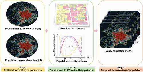
We proposed a spatiotemporal downscaling framework to map population dynamics with three key steps (Figure 1). First, we generated two baseline population maps during sleep time and work time (Section 3.1). Second, we derived urban functional zones and corresponding human activity patterns (Section 3.2). Finally, we estimated the hourly population distributions based on the baseline population and human activity patterns in urban functional zones (Section 3.3).

Figure 1. The framework of mapping temporal population dynamics.

3.1. Spatial downscaling of population

In step 1, two population maps during sleep and work times (Figure 2) were generated as baselines for further temporal downscaling in residential and other functional areas.

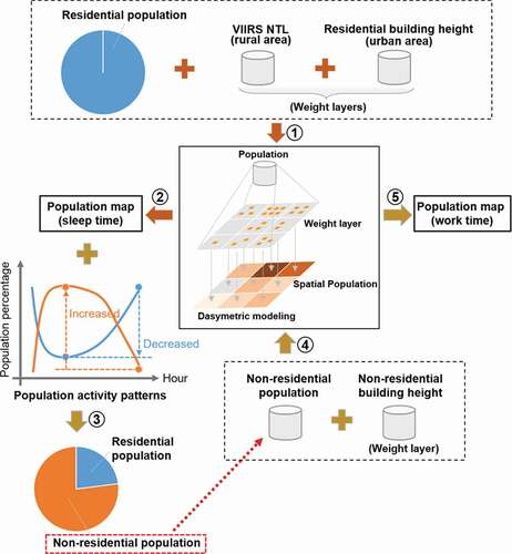
Figure 2. The workflow of generating baseline population maps during sleep and work times using the dasymetric method. From ① to ②generation of baseline population (sleep time) based on residential building height in urban areas and VIIRS NTL intensity in rural areas, respectively. From ③ to ⑤generation of baseline population (work time) based on nonresidential population and nonresidential building height.

3.1.1. Baseline population map during sleep time

We employed an effective dasymetric method to disaggregate census data into grids (Figure 2). Dasymetric mapping is an ancillary-driven method and was widely used in the spatial interpolation (Briggs et al. 2007; Mennis 2003). The dasymetric method introduces the density information from ancillary variables to redistribute the standardized data (e.g. census data) into a finer scale distribution. The critical step is the definition of weighting scheme and was usually determined by the existing or assumed relationship between the population and ancillary variables (Leyk et al. 2019). The census data were reallocated based on the weight to a finer scale population within the boundaries of each census unit.

In this paper, ① we combined the density information from residential BH and NTL intensity to characterize the distribution of population during sleep time in urban and rural areas, respectively (Supplementary Fig. S2). ② Schematic map of the dasymetric modeling work was based on two assumptions. Assumption one: in urban areas, the high residential BH can accommodate more people (validation in Supplementary Fig. S4 (a)). Assumption two: in underdeveloped rural areas, NTL intensity reflected the residence distribution across rural settlements. That is, the brighter the NTL was, the larger the population would be during sleep time. Based on these two assumptions, a snapshot of the baseline population map during sleep time was derived using Equation (1)(1) $W_i=\frac{p_i}{{\sum }_{i=1}^n{p}_i}$(1) and (2(2) $Po{p}_i=TP\times W_i$(2) ), representing the maximum of population in residential areas at the grid level for a regular weekday.

(1) $W_i=\frac{p_i}{{\sum }_{i=1}^n{p}_i}$(1)

(2) $Po{p}_i=TP\times W_i$(2)

where $p_i$ is the value of weight layer (BH or NTL intensity) at the $i$th pixel, $n$ is the total pixel number in a census unit, $W_i$ denotes the weight for reallocating population at the$i$th pixel,$TP$ is the total population in the census unit, and $Po{p}_i$ denotes the estimated population in the $i$th pixel.

3.1.2. Baseline population map during work time

The baseline population map during work time includes two parts: the remaining population in residential areas and the increased population in nonresidential areas in those pixels with mixed land uses. The increased population for each pixel was derived by disaggregating the total increased population in nonresidential areas using nonresidential BH (Supplementary Fig. S3) and the dasymetric method (Figure 2). During work time, the majority of people moved from residential areas into other functional zones involving diverse activities (e.g. work, study, entertainment, and shopping). According to the mobility patterns of human activities, we found a relatively high population percentage of 85%−100% in all functional zones in terms of active activities and the lowest percentage about 22% in residential zones at 11:00 am (details can be found in Section 3.2.2). ③ Therefore, given the purpose of delineating the maximum possible population in nonresidential zones, we calculated the decreased population from 0:00 to 11:00 in residential areas as the nonresidential population. ④ Thereafter, we reallocated this population into grids based on nonresidential BH with a similar assumption in Section 3.1.1., that is, high nonresidential BH can accommodate more people (validation in Supplementary Fig. S4 (b)). ⑤ Finally, we generated the baseline population map at work time by adding up the remaining population in residential areas and the newly increased population in nonresidential areas.

3.2. Urban functional zones (UFZ) and human activity patterns

3.2.1. Generation of UFZ

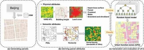
Urban functional zones were considered as the basic unit to further downscale two baseline population maps in temporal. We generated UFZ by integrating multi-source data using the framework with three steps (Figure 3). Detailed processes for generating UFZ in each step refer to the supplementary material S1.

Figure 3. Flow chart of generating urban functional zones (UFZ). Generating parcels (a); Deriving parcel attributes (b); and generation and accuracy evaluation of UFZ (c).

3.2.2. Estimation of general human activity patterns

We obtained a time series of population numbers for every UFZ from 7:00 to 0:00 using the UFZ and Baidu LBS data. Thereafter, a median statistical strategy was employed to estimate the general patterns for each activity type. However, given the characteristics of LBS data only recording the active user counts and there are almost no active users during sleep time, this dataset cannot be used to delineate the time series of population distribution in residential areas. Therefore, the population activity pattern in residential areas on weekday documented in (Greger 2015) was adopted in this study, which was also in line with our knowledge about population changes in residential areas across Beijing.

3.3. Temporal downscaling of population

We developed a temporal downscaling method based on human activity patterns and the corresponding urban functional zones. The derived population maps during work time ($t1$) and sleep time ($t2$) were used as the baselines of nonresidential and residential population, respectively (Figure 4). The population at grids during 7:00 − 0:00 was composed of two major components, that is, the population in UFZ and the population on the transportation networks. To be specific, the population of UFZ also consisted of two parts, and we denoted as static and active population. We considered the population in residential areas during hours of 7:00 − 0:00 to be the static population. Conversely, the population in the other functional types was denoted as the active population during this period. The difference between the population in UFZ and the official statistical population was the population on the roads.

Figure 4. Illustration of proposed framework for temporal population downscaling based on two baseline populations and population activity patterns. Note that the population on the road was changing over time.

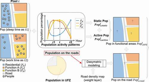
Specifically, we illustrated the downscaling process for a target pixel $i$ at time $t$ (Figure 4). First, the static population was calculated based on the population map at time $t2$ and the general human activity pattern in residential areas at time using Equation 3(3) $Po{p}_{i,static}^t=Po{p}_{i,t2}\times P_{i,Rres}^t$(3) . Second, the active population including people engaged in multiple activities (e.g. business, office, education, and recreation) was calculated based on the population at time and the general human activities in the corresponding nonresidential functional zones at time t using Equation 4(4) $Po{p}_{i,active}^t=\sum _{j=1}^{n}Po{p}_{i,t1}\times \frac{r_{i,j}}{{\sum }_{j=1}^n{r}_j}\times P_{i,j}^t;n=\left\{A,B\right\}$(4) . Third, the remaining population traveling on the roads was reallocated based on the road density using the dasymetric method in Equation 6. Given human activities in Beijing were mainly distributed within the 6^th ring area, we exploited ratios of the total populations during sleep time inside and outside the 6^th ring road ($R_{sleep}^{in\mathrm{\_}6th}$and$R_{sleep}^{out\mathrm{\_}6th}$; Equation 6(6) $Po{p}_i^t,road=\left\{\begin{array}{c}(Pop-Po{p}_{UFZ}^t)\times R_{sleep}^{in\mathrm{\_}6th}\times \frac{D_i}{\sum D},\\ ifiinsidethe{6}^{th}ringroad\\ (Pop-Po{p}_{UFZ}^t)\times R_{sleep}^{out\mathrm{\_}6th}\frac{D_i}{\sum D},\\ ifioutsidethe{6}^{th}ringroad\end{array}\right\}$(6) and 8(7) $R_{sleep}^{in\mathrm{\_}6th}=\frac{\sum Po{p}_{t2}^{in\mathrm{\_}6th}}{Pop}$(7) ) as reallocating coefficients to redistribute the rest of population into the grids. Finally, we derived the population map at the target time $t$ by aggregating these sub-type population (Equation 5(5) $Po{p}_{i,UFZ}^t=Po{p}_{i,static}^t+Po{p}_{i,active}^t$(5) and 9(8) $R_{sleep}^{in\mathrm{\_}6th}=\frac{\sum Po{p}_{t2}^{out\mathrm{\_}6th}}{Pop}$(8) ) at the pixel level.

(3) $Po{p}_{i,static}^t=Po{p}_{i,t2}\times P_{i,Rres}^t$(3)

(4) $Po{p}_{i,active}^t=\sum _{j=1}^{n}Po{p}_{i,t1}\times \frac{r_{i,j}}{{\sum }_{j=1}^n{r}_j}\times P_{i,j}^t;n=\left\{A,B\right\}$(4)

(5) $Po{p}_{i,UFZ}^t=Po{p}_{i,static}^t+Po{p}_{i,active}^t$(5)

(6) $Po{p}_i^t,road=\left\{\begin{array}{c}(Pop-Po{p}_{UFZ}^t)\times R_{sleep}^{in\mathrm{\_}6th}\times \frac{D_i}{\sum D},\\ ifiinsidethe{6}^{th}ringroad\\ (Pop-Po{p}_{UFZ}^t)\times R_{sleep}^{out\mathrm{\_}6th}\frac{D_i}{\sum D},\\ ifioutsidethe{6}^{th}ringroad\end{array}\right\}$(6)

(7) $R_{sleep}^{in\mathrm{\_}6th}=\frac{\sum Po{p}_{t2}^{in\mathrm{\_}6th}}{Pop}$(7)

(8) $R_{sleep}^{in\mathrm{\_}6th}=\frac{\sum Po{p}_{t2}^{out\mathrm{\_}6th}}{Pop}$(8)

(9) $Po{p}_i^t=Po{p}_{i,UFZ}^t+Po{p}_{i,road}^t$(9)

where $Po{p}_{i,t1}$ and $Po{p}_{i,t2}$ denote the population during work time and sleep time for ith pixel, respectively. $P_{i,Rres}^t$ and $P_{i,j}^t$ represent the population percentages of residential type and nonresidential functional type $j\left(j\in n\right)$, respectively. $r_{i,j}$ refers to the area ratio of functional type $j$ in $i$th pixel. Pop means the total population in 2015 in Beijing. $Po{p}_{i,UFZ}^t$ and $Po{p}_{UFZ}^t$ are the population in UFZ at time $t$ for ith pixel and the whole region, respectively. $R_{sleep}^{in\mathrm{\_}6th}$and$R_{sleep}^{out\mathrm{\_}6th}$ refer to the proportion of population distributed inside and outside the sixth ring road during sleep time, respectively. $D_i$ is the road density $i$th pixel. ${\sum }^D$ is the total road density in Beijing. $Po{p}_{t2}^{in\mathrm{\_}6th}$ and $Po{p}_{t2}^{out\mathrm{\_}6th}$ represent the sum of population inside and outside the sixth ring road, respectively.

4. Results and discussion

4.1. Baseline population maps

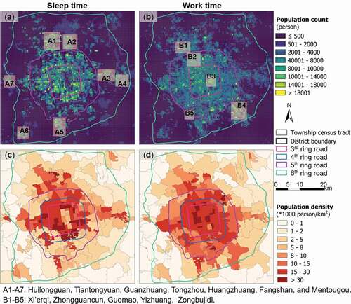
The spatial downscaling method of generating baseline population during sleep and work times can well capture the heterogeneity of population in spatial and the difference between sleep and work times (Figure 5). The spatial patterns of population show significant fluctuations between sleep time and work time. During sleep time, people are concentrated in the well-known “sleep town” (e.g. Huilongguan, Tiantongyuan, Guanzhuang, Tongzhou, and Huangzhuang), as shown in Figure 5a. Thereafter, the residential population moves to other places at work time. For example, the population in well-known working places increases (e.g. Xi’er qi, Zhongguancun, Guomao, Yizhuang, and Zongbujidi) in work time, as shown in Figure 5b. The population during work time is more dispersed throughout the interior area of the 5^th ring road compared with sleep time. Correspondingly, the population densities for most of the administrative streets inside the 5^th ring road are higher than at sleep time (Figure 5c and Figure 5d). In summary, the proposed framework of spatial downscaling enables us to characterize the distinct population patterns at these two base times.

Figure 5. Spatial patterns of derived baseline population maps. Populations during sleep time (a) and work time (b); Population density map at the administrative unit of level 4 during sleep time (c) and work time (d).

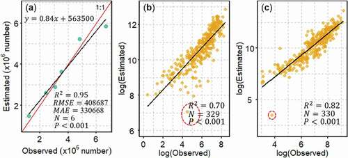
To further evaluate these two baseline population maps, we compared the results with population statistics for each ring area and the active users observed by the Baidu LBS dataset at an administrative unit of level 4, respectively (Figure 6). Figure 6a illustrates a good consistency (slope of 0.84 and R² of 0.95) between the estimated population and the census data during sleep time across ring areas. Besides, our results agree well with the observed Baidu LBS data that reflect the spatial distributions of active users with both R² higher than 0.70 (Figure 6b and Figure 6c). The underestimations for points with red circles are mainly due to the insufficient building footprints crawled from Baidu Maps in these regions. Overall, our proposed framework well characterizes the spatial distribution of population during sleep time and work time and can provide a basis for the next step of temporal downscaling.

Figure 6. Evaluation of derived baseline populations using the reference data. Comparison of the derived population with census data during sleep time across ring areas (a) and with Baidu LBS data collected at 0:00 at the administrative unit of level 4 (b); as well as the comparison of the derived population during work time with Baidu LBS data collected at 11:00 at the administrative unit of level 4 (c).

4.2. Urban functional zones

The results of accuracy assessment (the overall accuracy of 88.3%, the overall quantity disagreement of 0.03, and the overall allocation disagreement of 0.08) (Table 2) illustrate the optimized random forest performs well for categorizing urban functional zones (Pontius and Millones 2011; Foody 2020). Specifically, categories of education, office, open space and residence have the highest classification accuracy with both producer accuracy (PA) and user accuracy (UA) about 90%. Commercial and transportation categories show the lowest producer accuracy. The former is mistakenly recognized as office and residential areas, while the latter is mainly due to the small samples.

Table 2. Confusion matrix in categorizing UFZ.

Actual predicted	Com.	Edu.	Off.	Ope.	Rec.	Res.	Tra. ^#	Total	UA
Commercial	13	0	1	0	0	1	0	15	86.7%
Education	0	22	0	0	0	0	0	22	100%
Office	4	0	71	0	1	5	1	82	86.6%
Open space	0	0	0	34	1	0	0	35	97.1%
Recreation	0	1	1	0	12	1	0	15	80.0%
Residential	5	1	5	0	1	75	0	87	86.2%
Transportation	0	0	0	0	0	0	1	1	100%
Total	22	24	78	34	15	82	2	257
PA	59.1%	91.7%	91.0%	100%	80.0%	91.5%	50.0%		88.7%

Abbreviations: PA: producer’s accuracy. UA: user’s accuracy. # the transportation defined here only includes large public transportation hubs (e.g. railway station and airport).

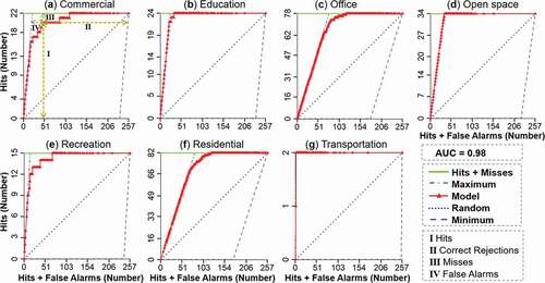
In addition, we evaluated the model performance using the total operating characteristic (TOC) approach based on continuous classification probabilities (Figure 7). As an improvement of the relative operating characteristic (ROC) that is popular in evaluating the performance of classifiers, the TOC curve can reveal information including four entries (e.g. hits, misses, false alarms, and correct rejections) for each threshold in visual (Pontius Jr and Si 2014; Ahmadlou et al. 2016). Under the curve (AUC) metric calculated by the area under the ROC curve, which is usually used to summarize the overall performance, is equal to the ratio of the area under the TOC curve within the parallelogram to the whole area of the parallelogram. We calculated the AUC using the averaging pairwise comparisons of classes (Hand and Till 2001). In summary, AUC of 0.98, which is greater than the random baseline AUC of 0.5, and TOC curves in the upper-left corner indicate a good performance of the RF model.

Figure 7. Total operating characteristic (TOC) for the performance of RF in the classification of UFZ. Note that the transportation class only includes large public transportation hubs (e.g. railway station and airport) in this paper.

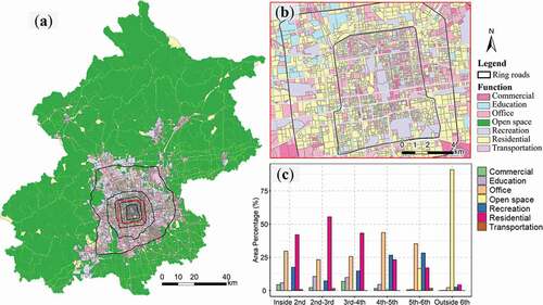
The majority of UFZ related to human activities except for open space are distributed within the 6^th ring road (Figure 8). Specifically, residential areas accounted for a large proportion of more than 40% inside the fourth ring road (Figure 8c). On the contrary, offices were mainly distributed in the 4^th to 6^th ring roads with the area proportions greater than 35%, followed by inside the 4^th ring road. The distribution of recreation areas was similar to the office. The commercial areas were mainly distributed inside the 4^th ring road, while the education areas were mainly distributed inside the 5^th ring areas. Open space was the largest categories outside of the 6^th ring road, with a value of 69.4%.

Figure 8. Urban functional zones of Beijing in 2015. An overview (a); close-up within the red box showing the city center of Beijing (b); area percentages of different functional types within each ring area (c).

4.3. Human activity patterns

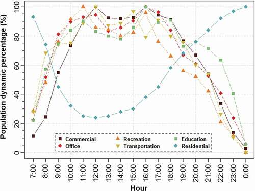
The estimated hourly activities show a distinct pattern between residential and other functional areas (Figure 9), and are consistent with other studies (Gu et al. 2018). These human activities patterns indicate the shift of population over time between multiple activity types. The changes of population can be approximated as a symmetrical structure. The population decreases rapidly during the morning commuting hours (7:00 − 9:00) in residential areas and reaches the lowest proportion from 11:00 − 13:00, accounting for about 24% of the population during the peak period (sleep time). Correspondingly, the population in areas of other functional types increased rapidly during this period and reached at a high proportion during work hours (10:00 − 17:00), along with the mobility of people from residential areas to engage in other daily activities (e.g. work, business, education, and leisure). Compared with the rapid changes of population proportions in the morning rush hours, the mobility of population from other types of functional zones into residential areas is relatively slower and lasts longer after working hours. To our current knowledge, this phenomenon is reasonable, considering the needs (e.g. entertainment and leisure) of people after getting off work.

Figure 9. The estimated patterns of human activities.

4.4. Evaluation of population dynamics

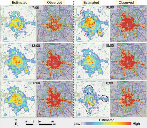
The spatial patterns of derived population dynamics show a good agreement with the patterns from the real-time Baidu heat maps (Figure 10), indicating that the proposed population downscaling framework can well characterize the spatial variabilities of population over time (Fig. S4). We took the hourly heat map snapshots collected from mobile Baidu Maps on 24 September 24 2020, as an example to illustrate the reliability of our results. It should be noted that there are some visual differences between our estimated and Baidu heat maps, due to the different way of visualizations (e.g. parameters and color). Despite these limitations, the estimated fluctuations of spatial population distribution over time are consistent with those from Baidu Maps. Specifically, the hotspots of population at working hours (e.g. 10:00) are mainly concentrated in the city center (inside or the area near the 5^th ring road, as circled by red color). This is consistent with the fact that those zones are the center of main commercial areas, working areas, and education. Population patterns change to sparsely distributed in residential areas at sleeping hours (e.g. 0:00, as circled as black in Figure 10). The spatial pattern of the population shows transitions during the morning (e.g. 7:00) and afternoon commuting (e.g. 18:00) hours.

Figure 10. Comparison of population heat maps between our estimations and that from Baidu Maps collected on 24 September 2020. Areas marked with red dash circles are aggregated nonresidential regions. Areas marked with black dash circles are aggregated residential regions.

4.5. Comparison with previous studies

This study developed a framework to downscale population at fine spatial and temporal scales by integrating census data with multi-source geospatial datasets. Compared with previous studies, our designed framework has advantages from three aspects. First, instead of “ambient population” of previous studies (Bhaduri et al. 2007), our proposed framework derived the time-specific spatial distributions of population, which can provide effective information for multiple applications (e.g. emergency planning, disaster-related evaluations, and human risks to environmental problems). Second, in the designed framework, we improved the strategy to capture the spatial heterogeneity of population during sleep time. The most popular used datasets, such as land cover/use, DEM and NTL (Panczak, Charles-Edwards, and Corcoran 2020), cannot accurately represent the distribution status of population. For example, although land use/cover datasets can express the distribution information of impervious surface related to population, they cannot express the detailed intensity information. Remotely observed NTL data can characterize the distribution of population. However, the direct usage of NTL data to map population could result in the underestimation in residential areas and overestimation in developed areas (e.g. commercial centers and transportation infrastructures). Because lights from residential areas are weakened or even non-existent due to the observation angles and transit times of satellites (i.e. 1:30 am for VIIRS satellite), while lights from commercial centers and traffic infrastructures have higher intensity and last longer. Considering the existing drawbacks of these datasets, we disaggregated census data into residential grids by combining residential BH data in urban areas and NTL data in rural areas. The derived population distribution during sleep time shows a good agreement both with our common knowledge of Beijing and with the observed distribution from the popular LBS platform of Baidu.

Third, this paper provides the hourly gridded population dataset on workdays at a 500 m resolution, and the proposed spatiotemporal downscaling framework is transferable to other regions. If we can obtain three elements (baselines, UFZ, and activity patterns) in a study area, we can use the proposed spatiotemporal downscaling framework to map population dynamics at specific hours. Two baseline population maps can be generated in other regions. The datasets used in this paper (NTL and BH) are widely available in other regions. The division of the spatial distribution of human activities can be easily implemented in other regions. Published datasets of functional zones in other cities can be directly used; otherwise, the method used in this study of generating urban functional zones can be easily replicated in other regions. The general activity patterns can be extracted from the LBS data collected in the target study area and replaced by the corresponding patterns. The use of general activity patterns alleviates the dependence on the real-time LBS dataset, which are costly and difficult to obtain, and helps future studies for estimating gridded population dynamics over large areas. Besides, this proposed framework is more robust and effective compared to studies with the direct use of LBS dataset. The use of general activity patterns mitigates the potential bias that could be introduced during the collection of LBS data (Song et al. 2019).

4.6. Limitations and uncertainties

Although our proposed framework provides an effective way to generate population dynamics at the grid level, there are still some limitations need further improvements due to the lack of “gold standard” data source for short-term population estimation. First, similar to previous studies, our evaluation of results derived from this spatiotemporal downscaling framework can be improved. A field survey is the most accurate manner for evaluation, although it is difficult to implement. It is challenging to verify the magnitude of the derived population at the pixel level, given that the reference LBS data are only a small proportion of the entire population. Second, the collected LBS data are still limited regarding the potential temporal changes in this paper. More data can be collected to capture the seasonal change of or weather effects on population activities. Our proposed framework can also be improved for population downscaling on weekends and holidays, when the data for capturing complicated human activity patterns and population flows inter-cities become available on these days (Gu et al. 2018). Third, although the dasymetric method is commonly used in population mapping, the direct use of ancillary variables might neglect the spatial heterogeneous relationship between variables and the population. Besides, the types of nonresidential buildings (e.g. commercial, office) could still be further classified to finely investigate this relationship if there are LBS data available to distinguish the number of users engaged in specific activities. In addition, this study assumed the total population of Beijing is a constant in a single year. We did not consider the temporary inflows or outflows (i.e. business travel and tourism), because the relevant datasets are not available and the mobility patterns for these groups are difficult to capture.

The use of human activity patterns in this study mitigates bias introduced by LBS data. However, there are still potential uncertainties due to the bias in data collecting (e.g. different preferences among age groups; no smart phone because of economic reason or for elderly; and the demanding change of location-based service over time) and the new collection time of LBS data compared with other data. In addition, the use of general pattern for each activity type might neglect the spatial heterogeneity between parcels with the same function. In summary, despite these uncertainties, this study still provides an insight to characterize the possible population dynamics, in the circumstance of difficulty to access the more detailed population flow information (i.e. outflow and inflow count) over time considering the privacy and security issues.

5. Conclusions

In this study, we developed a spatiotemporal downscaling framework to generate hourly population dynamics at a 500 m resolution by integrating multi-source geospatial datasets and took Beijing as an example to illustrate the processes and its effectiveness. Results from this proposed framework show a good agreement with the referenced population patterns collected from the real-time Baidu Maps. The distribution of population exhibits significant spatial heterogeneities and variabilities over time. During working hours (9:00 − 18:00), the population in Beijing is more homogenously distributed inside the 6^th ring area. In contrast, there are more clusters of high population during sleep hours (after 0:00). The population dynamic in hours except these two periods shows transitions.

The estimated population dynamics can serve as a valuable backbone for multiple applications, such as risk assessment for population involved in urban problems (Hu et al. 2017; Song et al. 2019). Compared to data with limited dynamic information, our high spatiotemporal population dataset has the potential for a more accurate estimation of population exposure to environmental issues, which is of great significance to explore the underlying mechanisms between environmental-related human diseases and various environmental problems (Song et al. 2019; Zhang, Zheng, and Chen 2019). In addition, this framework is transferable in other regions by integrating general human activity patterns and functional zones, providing the possibility of mapping population dynamics in a large area and for a long-term period. LBS datasets are still valuable sources to explore complicated spatiotemporal patterns of human activities and to map short-term population for current and future research. Further improvement can focus on the refinement of complicated human activities and the expansion of the dynamic population mapping to weekends and special periods (e.g. holidays and pandemic time) when the relevant data become available.

Acknowledgements

This work was supported by the National Key R&D Program of China under Grant [Number 2019YFE0126800]; and the program of China Scholarships Council (CSC) under Grant [Number 201906270221].

Disclosure Statement

The authors declare that they have no known competing financial interests or personal relationships that could have appeared to influence the work reported in this paper.

Supplementary material

Supplemental data for this article can be accessed here

Additional information

Funding

This work was supported by the National Key R&D Program of China [2019YFE0126800].