Google Earth Engine for large-scale land use and land cover mapping: an object-based classification approach using spectral, textural and topographical factors

ABSTRACT

Mapping the distribution and type of land use and land cover (LULC) is essential for watershed management. The Tigris-Euphrates basin is a transboundary region in the Middle East shared between six countries, but a recent fine-scale LULC map of the area is lacking. Using Landsat-8 time series, a 30-m resolution LULC map was produced for the Tigris-Euphrates basin. In total, 1184 Landsat scenes were processed within the Google Earth Engine (GEE). For the collection of ground truth data, differential manifestations of green cover were considered by dividing the study area into five climatic regions and the training samples were taken from each sub-region. To account for the temporal variation of LULC types, six two-month interval composite layers, including the spectral and thermal bands of Landsat-8, texture and spectral indices, as well as topographic factors were created for the target year 2019. Image segmentation and classification were performed using the simple non-iterative clustering (SNIC) and Random Forest (RF) algorithms, respectively. A computationally effective parallel processing approach was developed, which created a number of tiles and sub-tiles and a bulk command was converted into smaller parallel commands. The generated LULC map showed a satisfactory overall accuracy of 91.7%, with the highest User’s accuracy in water and wetland, and the lowest in rainfed crop and rangeland and the highest Producer’s accuracy in water and barren areas, and the lowest in garden and rangeland. This study highlights the necessity of using multi-temporal data for LULC mapping, in particular, multi-temporal NDVI, for the separation of different green cover types in arid and semi-arid environment.

KEYWORDS:

• Land use and land cover
• simple non-iterative clustering
• multi-temporal NDVI
• topographic data
• arid and semi-arid region mapping
• climate zones

1. Introduction

Land use and land cover (LULC) mapping has always been of interest to researchers, governments, and international organizations because of its association with ecological changes (Lambin and Meyfroidt 2010), socio-economic issues (Serra et al. 2014), hydrology (Breuer et al. 2009), climate change (Pielke 2005), and ecosystem services (Fei et al. 2018). The dynamic nature of LULC (Lambin, Geist, and Lepers 2003), however, entails the regular updating of LULC maps. The Tigris-Euphrates basin (TEB) is a vast transboundary basin of historical and international importance that is shared between six countries. In the past few decades, the basin has faced several environmental challenges and has been of strategic importance in terms of water resources. Understanding the distribution and current status of LULC types in this basin is essential for environmental studies and watershed management. Nevertheless, providing large-scale LULC maps is challenging, predominantly because of the heterogeneity of the environment and the spectral complexity of land surface on one hand, and by hardware and software limitations on the other. For example, to discern different LULC types, multi-temporal imagery is often required, but this solution gives rise to problems with data volume and processing time. Given the unprecedented rise in satellite imagery, substantial advances in satellite image processing, and the emergence of new platforms such as Google Earth Engine (GEE), it is critical to identify and propose solutions for the challenges of large-scale LULC mapping.

GEE is a powerful cloud-based platform for processing satellite imagery and providing geospatial data on a global scale. It provides an environment for a wide range of users where no prior knowledge about using supercomputers or large-scale commodity cloud computing services is needed (Gorelick et al. 2017). GEE is not only a multi-petabyte storage super database; it also provides advanced processing models and visualization tools. The use of GEE for various remote sensing applications such as wetland delineation (Amani et al., 2019; Mahdianpari et al. 2020a), LULC extraction (Zurqani et al. 2018; Ghorbanian et al. 2020), and crop mapping (Xiong et al. 2017; Gumma et al., 2020; Oliphant et al. 2019; Xie et al. 2019) has become prevalent in recent years. The application of GEE extends over a range of studies on the regional, continental, and global scales. Based on a time series of the normalized difference vegetation index (NDVI) from moderate resolution imaging spectroradiometer (MODIS) data, Xiong et al. (2017) extracted croplands for the African continent. Hansen et al. (2017) processed global Landsat data to characterize forest extent, loss, and gain during 2000–2012. Liu et al. (2018) processed Landsat images to map the global urban extent during 1990–2010 at five-year intervals. Based on Landsat data, Long et al. (2019) automatically identified burned areas on a global scale. For the first time, nationwide wetlands in Canada were mapped using multi-temporal Landsat-8 during 2016–2018 (Amani et al., 2019; Mahdianpari et al. 2020b). Irrigated croplands across the conterminous United States were mapped at a 30-m resolution using Landsat data from the beginning of 2011 to the end of 2012 (Xie et al. 2019). Cropland extent was mapped for Southeast and Northeast Asia using the time series of Landsat data (Oliphant et al. 2019). Liu et al. (2020) used Landsat imagery to map annual changes in urban extent on the global scale during 1985 to 2015.

In nearly all of the aforementioned studies, satellite images were processed using pixel-based classification. The pixel-based approach considers only the pixel values, whereas an object-based approach involves the segmentation of images into objects on multiple scales (Whiteside, Boggs, and Maier 2011). Object-based classification in large-scale studies decreases the computation time, because the number of segments is much smaller than the number of pixels. Segments are homogeneous, contiguous regions that are identified by one or more homogeneity indices in one or more dimensions (Blaschke 2010), and segmented images are then apportioned to the target classes using supervised or unsupervised classification algorithms (Belgiu and Csillik 2018). Recently, segmentation was provided within GEE, a process which uses the simple non-iterative clustering (SNIC) algorithm. Although segmentation in GEE is currently limited to the SNIC, it can be done outside GEE; the results are then returned for further processing.

The appropriate selection of input variables is one of the major steps of satellite image classification. For example, there are different types of green cover on the ground and separating them with a single set of variables from a specific date is unlikely. Multi-temporal data, however, allows classifiers to gain a deeper understanding of LULC characteristics, thus increasing classification accuracy (Zhang and Weng 2016). For example, considering the time series of NDVI can effectively capture the phenological pattern of various green covers (i.e. forest and rangeland) and their separation. In addition, texture and topographic factors increase the class separability (Lu and Weng 2007). Texture measurements provide spatial information on the values of neighboring pixels, which improves classification accuracy (Hall-Beyer 2017). However, these extra variables increase the volume of data and demand more processing time, if feasible. On the other hand, large-scale satellite image processing using GEE is still substantially time-consuming and often fails to execute when the number of input variables for classification increases. Parallel processing is an efficient way to make large-scale computation practical. It simultaneously executes a program which is divided into smaller sections on multiple processors to achieve greater speed. The basic idea is that the process of solving a problem can usually be divided into smaller sub-tasks which can be resolved in a shorter time by being performed simultaneously. In this regard, selecting the type of classification algorithm to be used to handle large-scale data in an appropriate amount of time is critical.

To date, a wide range of machine learning techniques have been implemented for satellite image processing, e.g. support vector machines (SVM) (Huang, Davis, and Townshend 2002; Shao and Lunetta 2012; Thanh Noi and Kappas 2018), RF (Oliphant et al. 2019; Xiong et al. 2017; Li and Xu 2020), and artificial neural networks (ANNs; Yuan, Van Der Wiele, and Khorram 2009; Song, Duan, and Jiang 2012). However, the RF algorithm has been increasingly used for LULC classification, as it efficiently handles high dimensional data, requires few tuning parameters, discovers complex patterns, and yields highly accurate results (Breiman 2001). GEE offers a number of classification algorithms, such as decision trees, RF, SVM, and the Naïve Bayes classifier; among these, RF is the most frequently used classification method (Tamomonia et al., 2020). As the current study used a large amount of spatiotemporal data, the RF algorithm was selected.

The current study aimed to generate a 30-m LULC map of the TEB using object-based classification and the RF algorithm on the GEE platform. As discussed above, most previous LULC mapping efforts have used pixel-based classification with limited input variables. In the present study, multi-temporal data was used, including spectral bands, texture, spectral indices, and topographic factors. Multi-temporal data was not used in previous large-scale studies within the GEE environment because of the computational time-out error which is addressed herein in the proposal of a parallel processing approach.

2. Study area

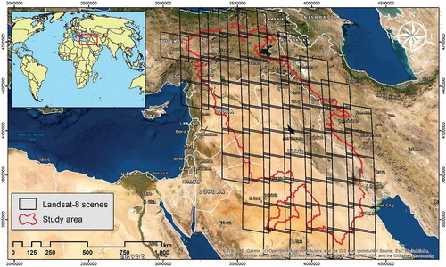
This study was performed on the TEB, which covers an area of about 806,232 km² and is shared between six countries: Iran, Iraq, Syria, Turkey, Saudi Arabia, and Kuwait. This region is one of the most important transboundary watersheds in the Middle East and is historically important as part of the Fertile Crescent. The Tigris and Euphrates river system, the main river system in West Asia, is located in this basin. The TEB is located in a humid, desert climate with an average monthly temperature between 6°C in January and 34°C in July (Al-Asadi 2017) and annual precipitation between 100 and 1,000 millimeters (Issa et al. 2013). The elevation of the basin varies from zero to 4400 meters above sea level; highlands are located in the northern parts of the area, and the southern regions include desert landforms. Figure 1 shows the location of the TEB on the world map. For a single date full coverage of the area, a total number of 75 Landsat scene are required.

Figure 1. Location of the TEB on the world map. The superimposed black frames are the footprint of Landsat 8 imagery

3. Data and methods

3.1 General steps of LULC mapping in the GEE environment

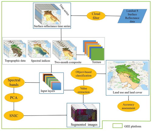
Figure 2 describes the general steps taken to create an LULC map of the TEB; the details of each step will be provided in subsequent sections. The classification process was divided into three major steps: data collection, segmentation, and classification. First, surface reflectance data for the target year 2019 was collected within GEE and divided into six two-month intervals starting from January-February to November-December. Next, gray-level co-occurrence matrices (GLCMs), spectral indices, and topographic factors were derived. In the second step, principle component analysis (PCA) was applied on the spectral bands of six two-month intervals to provide a basis for image segmentation using the SNIC algorithm. In the third step, image classification and accuracy assessment were performed using the RF algorithm and a confusion matrix, respectively.

Figure 2. Flowchart of the general process of LULC classification within the GEE environment

3.2. Classification scheme and ground truth data

In this paper, the classification scheme was defined as forest (including deciduous, evergreen, and mixed), rangeland (including shrubland and grassland), irrigated crop, rainfed crop (dry farming), garden (all types of horticulture and orchards), barren (deserts, dry salt flats, sandy fields, beaches, bare exposed rock), water (covering streams, lakes, reservoirs, bays, and estuaries), wetland (including wetland vegetation, lake marshes and floodplain wetlands), and artificial surfaces (all built-up areas including urban and rural settlements, transportation, mining, and industrial).

Ground truth samples were collected with the help of Google Earth imagery, Landsat NDVI time series, exploring the true and false color composites of the Landsat data, and expert knowledge. Ground truth samples were taken from different climate zones identified by Köppen-Geiger climate classification (Kottek et al. 2006; Rubel and Kottek 2010; Rubel et al. 2017), because large-scale areas contain different climatic zones which affect the phenological cycle of vegetation covers of different types. The Köppen-Geiger uses a combination of average annual and monthly temperatures and precipitation as well as seasonal precipitation to divide the study area into relatively homogeneous regions. It is grounded on the principle that native vegetation is the best indicator of climate; accordingly, the climatic boundaries of an area are determined by vegetation types (Kottek et al. 2006; Rubel and Kottek 2010; Rubel et al. 2017).

According to Cochran’s formula (Cochran 1953; Shetty 2019), the number of samples per LULC type were determined. Due to the extent and complexity of the environment, however, the number of samples was increased. The spatial distribution of samples was determined using a combination of random sampling and expert knowledge. Consistent with the object-oriented LULC classification, training samples were selected from the segments produced by the SNIC algorithm. Figure 3 shows the distribution of the collected samples over the climatic zones. Training samples are shown in green, and validation samples are shown in red. As seen in Table 1, a total of 10,488 samples from different classes were collected, of which 70% were used for training and 30% for the accuracy assessment. Because tree-based algorithms such as RF are sensitive to class imbalance, efforts were made to avoid large differences between the numbers of samples, although some classes such as wetlands covered a small area in the region, and relatively fewer samples were taken.

Figure 3. Distribution of training and test samples over the study area. Descriptions of climatic regions and their proportions in the study area are as follows: BSh: hot desert (17.55%), BWh: hot semi-arid (40.08%), Csa: monsoon-influenced humid subtropical climate (29.02%), Dfb: dry summer continental (0.55%), and Dsb: humid subtropical (12.77%)

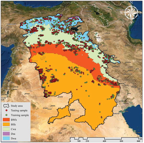
Table 1. Number of training and test samples for LULC classification

LULC type	Training (70%)	Test (30%)
Forest	891	387
Rangeland	1019	446
Irrigated crop	930	397
Rainfed crop	870	360
Garden	883	332
Barren	965	426
Water	659	303
Wetland	288	141
Artificial surfaces	816	375
Sum	7321	3167

3.3. Input data for classification

A time series of input variables was collected to characterize the training samples so as to differentiate between various LULC types. As shown in Table 2, a total of 105 input variables covering spectral bands, texture information, spectral indices, and topographic factors were used for the LULC mapping of the TEB in 2019. Except for the elevation and slope factors which are constant over time, the remaining variables were constructed as the average of the two months in which the mean of all the available data within the two months was computed.

Table 2. Input variables for RF algorithm to generate LULC map

Category	Description	Number of input variables	Temporal dimension	Total
Landsat-8 bands	blue, green, red, near infrared, SWIR1	7	6	42
	SWIR2, Thermal infrared band 10
Indices	NDVI, NDWI, TI, NBI	4	6	24
Terrain	Elevation, slope, slope-aspect	3	1	3
PCs GLCM	Angular Second Moment, Contrast,	9*4	1	36
	Correlation, Inverse Difference Moment, Sum Average,
	Sum Variance, Sum Entropy, Dissimilarity, Inertia
Total input variables				105

First, spectral bands comprising red, green, blue, near infrared (NIR), short wave IR (SWIR1 and 2), and brightness temperature based on band 10 were created for six two-month intervals in 2019 (42 variables). To keep the spatial consistency among the Landsat data, thermal bands were downscaled to the spatial resolution of the spectral bands. Then, using equations 1(1) $\mathrm{N}\mathrm{D}\mathrm{V}\mathrm{I}=\frac{NIR-R}{NIR+R}$(1) –4(4) $\mathrm{N}\mathrm{B}\mathrm{I}=\frac{Red\ast SWIR1}{NIR}$(4) , spectral indices including NDVI, normalized difference water index (NDWI) (Gao 1996), normalized difference tillage index (NDTI) (Daughtry et al. 2006), and new built-up index (NBI) (Zha et al., 2003) were calculated for the same six periods (24 variables).

(1) $\mathrm{N}\mathrm{D}\mathrm{V}\mathrm{I}=\frac{NIR-R}{NIR+R}$(1)

(2) $\mathrm{N}\mathrm{D}\mathrm{W}\mathrm{I}=\frac{Green-NIR}{Green+NIR}$(2)

(3) $\mathrm{N}\mathrm{D}\mathrm{T}\mathrm{I}=\frac{SWIR1-TIR\left(b10\right)}{SWIR1+TIR\left(b10\right)}$(3)

(4) $\mathrm{N}\mathrm{B}\mathrm{I}=\frac{Red\ast SWIR1}{NIR}$(4)

To consider texture information, a GLCM was applied, and a nine-layer image stack was created which accounted for contrast, correlation, inverse difference moment, sum average, sum variance, sum entropy, dissimilarity, inertia, and angular second moment. To calculate the GLCM, PCA was applied on the six two-month interval spectral bands, and the first four components of the PCA were separately fed to the GLCM; thus, for each component a nine-layer image stack was generated (36 variables). To calculate the texture, a GLCM with different kernel sizes was computed, and a kernel with the size of 5*5 pixels was employed. Topographic factors including elevation, slope, and slope-aspect were derived from the Shuttle Radar Topographic Mission (SRTM) digital elevation layer with the spatial resolution of 30 m (3 variables).

To estimate the area of each class properly, the input data was re-projected to Mollweide, which is an equal-area projection. In large-scale studies (e.g. Shafizadeh-Moghadam et al. 2019), the Mollweide projection can appropriately estimate the true area.

3.4. Image segmentation

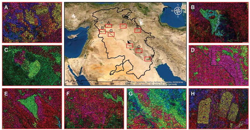
Image segmentation was implemented within the GEE environment based on the SNIC algorithm. The main parameters of SNIC are the “compactness factor” which affects the shape of clusters (the larger the values the more compact clusters are produced); the “connectivity” which defines the type of contiguity to merge adjacent clusters (queen: 4 or rook: 8); and a “neighborhoodSize” to avoid tile boundary artifacts. Considering the characteristics of the study area, these parameters were experimentally set as follows: compactness = 0.5, connectivity = 8, and neighborhood size = 128.Belgiu and Csillik (2018) used red, green, blue, and NIR from several periods as input for image segmentation; however, their classification scheme was solely crop mapping. In the current study, PCA was applied on six sets of two-month interval spectral data in 2019, including red, green, blue, NIR, SWIR1 and 2, and brightness temperature. Studies have shown that entering highly-correlated variables reduces the performance of models (Kuhn and Johnson 2013). Based on the scree-plot, the first four PCs were selected as the input of SNIC for image segmentation, accounting for over 95% of the variance. Figure 4 shows the output of the SNIC algorithm, which is the segmentation of the Landsat data. In order to better display the image, some parts have been selected and enlarged.

Figure 4. Image segmentation using the SNIC algorithm

3.5. Random Forest (RF)

The RF algorithm was used for LULC classification of the TEB in 2019. Prior to classification, eleven variables which had near zero variance were identified and excluded (Kuhn and Johnson 2013). Thus, LULC classification was conducted using 94 variables. The segmented images produced by the SNIC algorithm were overlaid on the pixel-based layers, and the mean pixel values were extracted for each segment. Then, the RF algorithm was applied on the segmented images for LULC classification.

RF provides a variable importance metric, is resistant to outliers, and is capable of handling high dimensional data and discovering non-linear relationships (Breiman 2001). RF is composed of many implementations of a base learner called classification and regression tree (CART) (Breiman 2001). Each CART is constructed using bootstrap sampling by which a subset of samples is used for training (in-bag), and the out-of-bag samples are used for internal cross validation (Breiman 2001). The number of trees for the RF was set to 500, and the mtry was set as the square root of the input variables. To construct each tree, mtry refers to the number of input variables randomly sampled for splitting at root node. One of the advantages of the RF algorithm is the prioritization of input variables in the task of LULC classification. The RF algorithm operates in such a way that input variables with lower discriminative ability have a very low chance of being selected; therefore, the RF is effective at excluding inefficient variables. In this paper, variable importance refers to the mean decrease in accuracy, which shows the degree of accuracy the model loses by eliminating each variable. The structure of the RF algorithm, which is based on tree-based models, is such that it considers the interactions among the input variables. Therefore, the importance of input variables is relative, and together, they lead to the classification process.

3.6. Parallel processing in the GEE environment

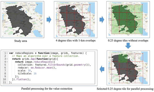
Due to the immense extent of the study area and the large size of the Landsat time series, GEE was not able to process the entire region at once. Therefore, considering the size of the stacked layers, the study area was experimentally divided into 4-degree tiles (Figure 5). Using 4-degree tiles with an overlap of 1 km, the whole area was divided into 16 tiles. The overlap of the tiles ensures complete coverage of the area in the mosaicking process of the final map. The value extraction of input variables for several million segments for each of the 4-degree tiles could not be done all at once in GEE; hence, 4-degree tiles were further sub-divided into smaller–sized tiles (0.25 degrees without overlap). In practice, the process was done by dividing a bulk command into smaller parallel commands. This method receives multiple input arguments, including a stacked image, 0.25 degree sub-tiles, and a segment vector. Next, using the mean reducer, it extracts values from the stacked image, which are then sent to the GEE server for further processing, and ultimately the results of all commands are merged. The joint part of the adjacent tiles is taken from the tile that is called first.

Figure 5. Schematic representation of parallel processing to prevent computational time-out error

4. Results

4.1. Classification variable importance

Figure 6 shows the variable importance in the LULC mapping of the TEB. To facilitate visualization, only the top ten variables out of 95 input variables were considered for display. As can be seen, the elevation, three spectral indices including NDVI, NDWI, NDTI, the SWIR1, and the correlation parameter from the GLCM are among the ten most important input variables. Of note is the temporal effect of the spectral indices; for example, the temporal effect of NDVI was prominent. NDVI was selected in five periods of the year from January to October and not selected only in the last two months of the year, November and December, because during these months, greenness is minimum. The NDVI time series played a key role in separating different vegetation types, because the growing season of annual and evergreen vegetation covers showed discernible patterns of NDVI. Along with spectral bands and indices, topographic derivatives such as elevation were critical in class separation and were ranked as the first or the second most important variable for most classes.

Figure 6. The importance of input variables to create a LULC map of the TEB using the RF algorithm. The horizontal axis represents the relative importance of input variables, and T1 to T6 in the vertical axis represent the months of the year as two-month intervals from January to December

4.2. Accuracy assessment of the LULC map of the TEB

Figure 7 shows the LULC map of the TEB in 2019. As seen, the northern half is mostly covered by rangeland, and the southern half is mostly barren and irrigated crop land. Barren parts are located mainly in Iraq and Syria, and rangelands are located in Turkey. Table 3 shows that barren and rangeland are the largest LULC types accounting for 46.46% and 20.87% of the TEB, respectively. Irrigated crop and rainfed crop share 24.29%, and garden accounts for 1.29%. Over 4.29% of the TEB is forest, while water and wetland comprise 1.56%, and 1.24% is artificial surfaces. The generated LULC map was visually and statistically evaluated using Google Earth imagery and a confusion matrix, respectively. To better display the details, several areas were selected and compared with their equivalent Google Earth images. Visual interpretation and comparison with high-resolution satellite images revealed that object-based classification using the RF algorithm delineated the LULC classes accurately and provided a visually satisfactory depiction of nearly all classes. Statistical evaluation of the LULC map was conducted using 30% of the ground truth data (validation set) that was not used in classification. Since the Kappa index has been found to be misleading for practical remote sensing applications (Pontius and Millones 2011; Foody 2020), the classified map was assessed using a confusion matrix with overall accuracy, producer’s accuracy (PA), and user’s accuracy (UA) (Olofsson et al. 2014). As seen in Table 4, the overall accuracy was 91.7%; the highest UA (or lowest commission error) was for water and wetland, and the lowest UA (or highest commission error) was for the rainfed crop and rangeland categories. The highest PA (or lowest omission error) was for water and barren areas, and the lowest PA (or highest omission error) was for the garden and rangeland categories.

Figure 7. The 30-m Landsat-derived LULC map for the nominal year 2019 for the TEB (upper panel). Visual assessment of a few sample locations labeled A-D (middle panel) against a natural color composite of high resolution Google Earth imagery (lower panel)

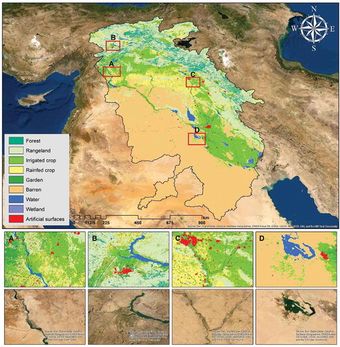
Table 3. Area and percentage of each land use and land cover type in the TEB in 2019

LULC type	Area (km^2)	Percentage of the study area
Forest	34,622	4.29
Rangeland	168,259	20.87
Irrigated crop	137,543	17.06
Rainfed crop	58,251	7.23
Garden	10,433	1.29
Barren	374,551	46.46
Water	10,785	1.34
Wetland	1794	0.22
Artificial surfaces	9994	1.24
Sum	806,232	100

Table 4. Confusion matrix for the generated LULC map of the TEB. Columns represent reference data, and rows represent the mapped classes

LULC type	Forest	Rangeland	Irrigated crop	Rainfed crop	Garden	Barren	Water	Wetland	Artificial surfaces	UA
Forest	355	26	1	1	4	0	0	0	0	0.872
Rangeland	19	394	2	25	1	4	0	0	1	0.867
Irrigated crop	0	2	358	15	19	1	0	0	2	0.906
Rainfed crop	0	21	9	323	4	0	0	0	3	0.845
Garden	33	6	16	8	267	0	0	0	2	0.875
Barren	0	0	0	1	0	424	0	0	1	0.986
Water	0	0	1	0	0	0	302	0	0	1
Wetland	0	0	3	0	0	1	0	137	0	1
Artificial surfaces	0	5	5	9	10	0	0	0	346	0.974
PA	0.917	0.883	0.901	0.897	0.804	0.995	0.996	0.971	0.922	0.917

5. Discussion

5.1. Object-based LULC classification of the TEB using the Random Forest algorithm

In this study, a 30-m resolution LULC map of the TEB for the target year 2019 was generated. The TEB is a vast transboundary region in the Middle East which is critically important from the socioeconomic, hydro–political, and environmental aspects. Extensive agricultural activities, unprecedented dam construction, and water and environmental disputes are among the main issues in the TEB that are closely related to the LULC maps. This map provides an updated view of the extent and distribution of different LULC types using the RF algorithm, which is of great importance for the effective watershed management.

Ensemble algorithms such as the RF have appeared as potentially more accurate and stable alternatives to parametric models (e.g. maximum likelihood) and individual decision trees (Rodriguez-Galiano et al. 2012; Chen et al. 2014). The RF algorithm efficiently operates on large datasets and multi-dimensional data, which was the case in this study, and a critical aspect for analyzing remote sensing data (Jensen 2015). Unlike the majority of previous studies that adopted a pixel-based approach for LULC mapping within the GEE environment (Amani et al., 2019; Long et al. 2019; Xie et al. 2019), the current study used an object-based approach. Tamiminia et al. (2020) observed that the object-based methods within GEE produced more accurate classifications than pixel-based methods, furthermore, object-based classification reduces processing time considerably. Recently, Ghorbanian et al. (2020) used the RF algorithm for pixel-based LULC mapping in Iran and employed object-based classification and a majority voting within each segment in a post-processing step to enhance the accuracy of their results. This approach leads to the removal of isolated pixels and small patches that occur in pixel-based classification. In contrast to Ghorbanian et al. (2020), the current study first employed the SNIC algorithm for image segmentation and then used the RF to classify the segmented images.

5.2. Parallel processing and tiling within Google Earth Engine

The use of multi-temporal input variables and inclusion of ancillary variables increase computational costs and result in computation time out error. Previous studies (e.g. Amani et al., 2019; Ghorbanian et al. 2020) reported computational encumbrance as a deterrent within the GEE environment which prevented the inclusion of texture and spectral indices. The reason for this is that the GEE cloud computing platform has a limited processing volume for each user. GEE considers a limited amount of RAM per process, and a large volume of satellite imagery cannot be processed all at once. This study proposed a hierarchical parallel processing that divided huge volumes of data into small parallel commands, and eventually, the outputs of all commands were merged. Parallel processing was first used to extract the values of independent variables for the segmented images. Then, the classifier was calibrated using the training data collected from the whole region, and again using the parallel processing, the calibrated classifier was applied on the prespecified tiles individually. This approach created a seamless LULC map when the tiles were mosaicked. As an alternative, each climatic zone was classified independently, and the final classification map of the study area was a composite of the individual climatic zone classifications. This approach, based on the calibration of each climatic zone separately using its own training data, revealed that the mosaicked map at the edge of overlapping grids was inconsistent because of the differences in training set selection for individual climatic zones that produced different spectral classes on either side of climatic zone boundaries. As a result, the LULC map showed abrupt changes along the boundaries of the overlapping areas. Therefore, the first approach is recommended.

5.3. Multi-temporal variables and sampling in large-scale areas

Multi-temporal variables account for the dynamic characteristics of LULC types for image classification (Oliphant et al. 2019; Phalke et al. 2020). Nevertheless, spectral bands are not enough to separate different LULC types, mainly due to the spectral similarity of vegetation types and the spatial heterogeneity of impervious surfaces (Gong et al. 2016). In addition to the spectral bands, this study applied texture information, spectral indices including NDVI, NDWI, NBI and NDTI, and topographic factors. Variable importance extracted by the RF algorithm revealed the necessity of using multi-temporal data for LULC mapping. The results also showed that the multi-temporal NDVI played an influential role in the separation of different LULC types, while NIR and red bands were absent from the top ten important input variables, because the influence of these two bands was reflected in the NDVI. Nevertheless, to improve the quality of LULC classification, particularly in large-scale studies with heterogeneous environments, including further ancillary data such as soil types is necessary.

Regardless of the type of classification algorithm and selection of input variables, taking other considerations into account such as providing representative samples plays a key role in boosting the accuracy of the generated LULC maps. Prior to ground truth collection, signature extension over space and time have to be fully explored (Jia et al. 2014). In other words, the spatiotemporal homogeneity of the environmental and climatic conditions of the study area have to be considered. Depending on the purpose of classification, geographical stratification is an efficient approach for finding homogeneous areas and for sampling inside each stratum. In large scale areas, particularly when the predominant surface cover is vegetation, it is crucial to have basic information such as the beginning, duration, and end of the growing season. Since the phenological characteristics of vegetation are affected by climatic conditions, collecting ground truth data in a way that covers different climatic regions is necessary for having representative samples. For this reason, the study area in this research was stratified using the climate zones identified by Köppen-Geiger climate classification, and ground truth data was taken from each zone. Nevertheless, ground truth data collection to identify training samples in large-scale studies remains challenging, particularly in remote and inaccessible areas. Volunteered geographic information (VGI) data such as OpenStreetMap (OSM) could act as a complementary data source in future studies.

5.4. Accuracy assessment and confusion of different LULC types

The results of the LULC classification of the TEB showed an overall accuracy of 91.7%. This figure may be inflated, however, due to spatial autocorrelation among the ground truth data. The presence of a positive spatial autocorrelation among the contiguous or adjacent pixels means that nearby pixels probably have similar brightness values (Jensen 2015). In this situation, traditional random cross-validation techniques may lead to the overestimation of a model’s accuracy (Valavi et al. 2019). While conventional cross-validation approaches are pervasive in the literature, the inclusion of spatial cross-validation in future studies can provide a better estimation of model performance.

As seen in this paper, despite the relatively high overall accuracy of the LULC map, some LULC types showed class confusion. Spatial proximity and spectral similarity may explain this result. Clear-cut classes in the study area are sporadic, and landscape patterns are complex and composed of gradients between the classes. For example, gradient or a mixture of forest and rangeland was often observed. Also, the adjacency of garden to forest, especially in some valleys in the northern region, caused some confusion of these two LULC types. The confusion matrix revealed a mix-up between the rangeland and rainfed crop and a lower accuracy compared to the other LULC types. A time series examination of the NDVI index indicated that rangeland and rainfed crop had close phenological patterns, and their maximum NDVI was almost identical. One of the issues that give rise to the class confusion was related to the minor differences in the temporal patterns of NDVI for vegetation covers that can be captured through a dense time series of NDVI, such as using MODIS-based NDVI. Moreover, expert knowledge can be applied to enhance the quality of the classification map through rule-based algorithms, such as CART, in the post-classification process.

6. Conclusions

The current results demonstrated the efficiency of multi-temporal Landsat 8, texture information, spectral indices, and topographic derivatives for LULC mapping. Due to the vast expanse of the study area and so as to account for the effect of temperature and precipitation on the phenological patterns, training samples were taken from different climatic zones. To overcome the computation error of GEE in handling the massive amount of data, a parallel processing approach was proposed which was computationally efficient. Parallel processing allowed the inclusion of multi-temporal data, which helped to boost the separability of different LULC types. Using the RF algorithm, the most important input variables used to demarcate different LULC types were identified, highlighting the importance of considering multi-temporal input for classification. The produced LULC map shows that rangeland, barren, and cropland are the dominant LULC types of the TEB. The diversity and complexity of LULC types are evident in the northern half of the basin, while the southern half is mainly composed of barren areas. The accuracy of the classified map was assessed both visually and statistically and had an overall accuracy of 91.7%, which is satisfactory.

In this paper, a large number of variables were considered and we were faced with a high-dimensional feature space; hence, feature selection techniques are recommended for the future studies. This is because when the number of variables increases, the complexity of learning models such as the RF algorithm increases. Furthermore, as SNIC is currently the only segmentation algorithm within the GEE environment, the implementation of other methods, such as multi-resolution segmentation, is also suggested.

Research highlights

• A 30-m resolution LULC map of the Tigris-Euphrates basin was generated

• Collection of training data from different climatic zones crucial in arid regions

• A parallel processing approach was developed in the GEE platform

• Significance of multi-temporal features collection was confirmed

• Segmentation and classification was performed using the SNIC and RF algorithms

Disclosure statement

No potential conflict of interest was reported by the author(s).

References

- Al-Asadi, S. A. 2017. “The Future of Freshwater in Shatt Al-Arab River (Southern Iraq).” Journal of Geography and Geology 9 (2): 24–38. doi:https://doi.org/10.5539/jgg.v9n2p24.
- Amani, M., S. Mahdavi, M. Afshar, B. Brisco, W. Huang, M. J. M. S., C. Hopkinson, S. Banks, J. Montgomery, and C. Hopkinson. 2019. “Canadian Wetland Inventory Using Google Earth Engine: The First Map and Preliminary Results.” Remote Sensing 11 (7): 842. doi:https://doi.org/10.3390/rs11070842.
- Belgiu, M., and O. Csillik. 2018. “Sentinel-2 Cropland Mapping Using Pixel-based and Object-based Time-weighted Dynamic Time Warping Analysis.” Remote Sensing of Environment 204: 509–523. doi:https://doi.org/10.1016/j.rse.2017.10.005.
- Blaschke, T. 2010. “Object Based Image Analysis for Remote Sensing.” ISPRS Journal of Photogrammetry and Remote Sensing 65 (1): 2–16. doi:https://doi.org/10.1016/j.isprsjprs.2009.06.004.
- Breiman, L. 2001. “Random Forests.” Machine Learning 45 (1): 5–32. doi:https://doi.org/10.1023/A:1010933404324.
- Breuer, L., J. A. Huisman, P. Willems, H. Bormann, A. Bronstert, B. F. W. Croke, … G. Kite. 2009. “Assessing the Impact of Land Use Change on Hydrology by Ensemble Modeling (LUCHEM). I: Model Intercomparison with Current Land Use.” Advances in Water Resources 32 (2): 129–146. doi:https://doi.org/10.1016/j.advwatres.2008.10.003.
- Chen, W., X. Li, Y. Wang, G. Chen, and S. Liu. 2014. “Forested Landslide Detection Using LiDAR Data and the Random Forest Algorithm: A Case Study of the Three Gorges, China.” Remote Sensing of Environment 152: 291–301. doi:https://doi.org/10.1016/j.rse.2014.07.004.
- Cochran, W. G. (1953). “Sampling Techniques.” doi:https://doi.org/10.2307/1268167
- Daughtry, C. S., P. C. Doraiswamy, E. R. Hunt Jr, A. J. Stern, J. E. McMurtrey Iii, and J. H. Prueger. 2006. “Remote Sensing of Crop Residue Cover and Soil Tillage Intensity.” Soil and Tillage Research 91 (1–2): 101–108.
- Fei, L., Z. Shuwen, Y. Jiuchun, C. Liping, Y. Haijuan, and B. Kun. 2018. “Effects of Land Use Change on Ecosystem Services Value in West Jilin since the Reform and Opening of China.” Ecosystem Services 31: 12–20. doi:https://doi.org/10.1016/j.ecoser.2018.03.009.
- Foody, G. M. 2020. “Explaining the Unsuitability of the Kappa Coefficient in the Assessment and Comparison of the Accuracy of Thematic Maps Obtained by Image Classification.” Remote Sensing of Environment 239: 111630. doi:https://doi.org/10.1016/j.rse.2019.111630.
- Gao, B. C. 1996. “NDWI—A Normalized Difference Water Index for Remote Sensing of Vegetation Liquid Water from Space.” Remote Sensing of Environment 58 (3): 257–266. doi:https://doi.org/10.1016/S0034-4257(96)00067-3.
- Ghorbanian, A., M. Kakooei, M. Amani, S. Mahdavi, A. Mohammadzadeh, and M. Hasanlou. 2020. “Improved Land Cover Map of Iran Using Sentinel Imagery within Google Earth Engine and a Novel Automatic Workflow for Land Cover Classification Using Migrated Training Samples.” ISPRS Journal of Photogrammetry and Remote Sensing 167: 276–288. doi:https://doi.org/10.1016/j.isprsjprs.2020.07.013.
- Gong, P., L. Yu, C. Li, J. Wang, L. Liang, X. Li, Z. Zhu, Y. Bai, Y. Cheng, and Z. Zhu. 2016. “A New Research Paradigm for Global Land Cover Mapping.” Annals of GIS 22 (2): 87–102. doi:https://doi.org/10.1080/19475683.2016.1164247.
- Gorelick, N., M. Hancher, M. Dixon, S. Ilyushchenko, D. Thau, and R. Moore. 2017. “Google Earth Engine: Planetary-scale Geospatial Analysis for Everyone.” Remote Sensing of Environment 202: 18–27. doi:https://doi.org/10.1016/j.rse.2017.06.031.
- Gumma, M. K., P. S. Thenkabail, P. G. Teluguntla, A. Oliphant, J. Xiong, C. Giri, A. M. Whitbread, S. Dixit, and A. M. Whitbread. 2020. “Agricultural Cropland Extent and Areas of South Asia Derived Using Landsat Satellite 30-m Time-series Big-data Using Random Forest Machine Learning Algorithms on the Google Earth Engine Cloud.” GIScience & Remote Sensing 57 (3): 302–322. doi:https://doi.org/10.1080/15481603.2019.1690780.
- Hall-Beyer, M. 2017. “Practical Guidelines for Choosing GLCM Textures to Use in Landscape Classification Tasks over a Range of Moderate Spatial Scales.” International Journal of Remote Sensing 38 (5): 1312–1338. doi:https://doi.org/10.1080/01431161.2016.1278314.
- Hansen, M. C., P. V. Potapov, R. Moore, M. Hancher, S. A. Turubanova, A. Tyukavina, … J. R. G. Townshend. 2017. “High-resolution Global Maps of 21st-century Forest Cover Change (2013) Science, 342.” Accessed 24: 850–853.
- Huang, C., L. S. Davis, and J. R. G. Townshend. 2002. “An Assessment of Support Vector Machines for Land Cover Classification.” International Journal of Remote Sensing 23 (4): 725–749. doi:https://doi.org/10.1080/01431160110040323.
- Issa, I., N. Al-Ansari, G. Sherwany, and S. Knutsson. 2013. “Trends and Future Challenges of Water Resources in the Tigris–Euphrates Rivers Basin in Iraq.” Hydrology and Earth System Sciences Discussions 10: 14617–14644.
- Jensen, J. R. 2015. Introductory Image Processing: A Remote Sensing Perspective. 4th ed. Pearson.
- Jia, K., S. Liang, N. Zhang, X. Wei, X. Gu, X. Zhao, X. Xie, and X. Xie. 2014. “Land Cover Classification of Finer Resolution Remote Sensing Data Integrating Temporal Features from Time Series Coarser Resolution Data.” ISPRS Journal of Photogrammetry and Remote Sensing 93: 49–55. doi:https://doi.org/10.1016/j.isprsjprs.2014.04.004.
- Kottek, M., J. Grieser, C. Beck, B. Rudolf, and F. Rubel. 2006. “World Map of the Köppen-Geiger Climate Classification Updated.” Meteorologische Zeitschrift 15 (3): 259–263. doi:https://doi.org/10.1127/0941-2948/2006/0130.
- Kuhn, M., and K. Johnson. 2013. Applied Predictive Modeling (Vol. 26). New York, NY: Springer.
- Lambin, E. F., H. J. Geist, and E. Lepers. 2003. “Dynamics of Land-use and Land-cover Change in Tropical Regions.” Annual Review of Environment and Resources 28 (1): 205–241. doi:https://doi.org/10.1146/annurev.energy.28.050302.105459.
- Lambin, E. F., and P. Meyfroidt. 2010. “Land Use Transitions: Socio-ecological Feedback versus Socio-economic Change.” Land Use Policy 27 (2): 108–118. doi:https://doi.org/10.1016/j.landusepol.2009.09.003.
- Li, K., and E. Xu. 2020. “Cropland Data Fusion and Correction Using Spatial Analysis Techniques and the Google Earth Engine.” GIScience & Remote Sensing 57 (8): 1026–1045. doi:https://doi.org/10.1080/15481603.2020.1841489.
- Liu, X., G. Hu, Y. Chen, X. Li, X. Xu, S. Li, S. Wang, and S. Wang. 2018. “High-resolution Multi-temporal Mapping of Global Urban Land Using Landsat Images Based on the Google Earth Engine Platform.” Remote Sensing of Environment 209: 227–239. doi:https://doi.org/10.1016/j.rse.2018.02.055.
- Liu, X., Y. Huang, X. Xu, X. Li, X. Li, P. Ciais, … P. Gong. 2020. “High-spatiotemporal-resolution Mapping of Global Urban Change from 1985 to 2015.” Nature Sustainability 3: 564–570.
- Long, T., Z. Zhang, G. He, W. Jiao, C. Tang, B. Wu, R. Yin, G. Wang, and R. Yin. 2019. “30 M Resolution Global Annual Burned Area Mapping Based on Landsat Images and Google Earth Engine.” Remote Sensing 11 (5): 489. doi:https://doi.org/10.3390/rs11050489.
- Lu, D., and Q. Weng. 2007. “A Survey of Image Classification Methods and Techniques for Improving Classification Performance.” International Journal of Remote Sensing 28 (5): 823–870. doi:https://doi.org/10.1080/01431160600746456.
- Mahdianpari, M., B. Brisco, J. E. Granger, F. Mohammadimanesh, B. Salehi, S. Banks, Q. Weng, L. Bourgeau-Chavez, and Q. Weng. 2020a. “The Second Generation Canadian Wetland Inventory Map at 10 Meters Resolution Using Google Earth Engine.” Canadian Journal of Remote Sensing 46 (3): 360–375. doi:https://doi.org/10.1080/07038992.2020.1802584.
- Mahdianpari, M., H. Jafarzadeh, J. E. Granger, F. Mohammadimanesh, B. Brisco, B. Salehi, Q. Weng, and Q. Weng. 2020b. “A Large-scale Change Monitoring of Wetlands Using Time Series Landsat Imagery on Google Earth Engine: A Case Study in Newfoundland.” GIScience & Remote Sensing 57 (8): 1102–1124. doi:https://doi.org/10.1080/15481603.2020.1846948.
- Oliphant, A. J., P. S. Thenkabail, P. Teluguntla, J. Xiong, M. K. Gumma, R. G. Congalton, and K. Yadav. 2019. “Mapping Cropland Extent of Southeast and Northeast Asia Using Multi-year Time-series Landsat 30-m Data Using a Random Forest Classifier on the Google Earth Engine Cloud.” International Journal of Applied Earth Observation and Geoinformation 81: 110–124.
- Olofsson, P., G. M. Foody, M. Herold, S. V. Stehman, C. E. Woodcock, and M. A. Wulder. 2014. “Good Practices for Estimating Area and Assessing Accuracy of Land Change.” Remote Sensing of Environment 148: 42–57. doi:https://doi.org/10.1016/j.rse.2014.02.015.
- Phalke, A. R., M. Özdoğan, P. S. Thenkabail, T. Erickson, N. Gorelick, K. Yadav, and R. G. Congalton. 2020. “Mapping Croplands of Europe, Middle East, Russia, and Central Asia Using Landsat, Random Forest, and Google Earth Engine.” ISPRS Journal of Photogrammetry and Remote Sensing 167: 104–122. doi:https://doi.org/10.1016/j.isprsjprs.2020.06.022.
- Pielke, R. A. 2005. “Land Use and Climate Change.” Science 310 (5754): 1625–1626. doi:https://doi.org/10.1126/science.1120529.
- Pontius, R. G., Jr, and M. Millones. 2011. “Death to Kappa: Birth of Quantity Disagreement and Allocation Disagreement for Accuracy Assessment.” International Journal of Remote Sensing 32 (15): 4407–4429. doi:https://doi.org/10.1080/01431161.2011.552923.
- Rodriguez-Galiano, V. F., M. Chica-Olmo, F. Abarca-Hernandez, P. M. Atkinson, and C. Jeganathan. 2012. “Random Forest Classification of Mediterranean Land Cover Using Multi-seasonal Imagery and Multi-seasonal Texture.” Remote Sensing of Environment 121: 93–107. doi:https://doi.org/10.1016/j.rse.2011.12.003.
- Rubel, F., K. Brugger, K. Haslinger, and I. Auer. 2017. “The Climate of the European Alps: Shift of Very High Resolution Köppen-Geiger Climate Zones 1800–2100.” Meteorologische Zeitschrift 26 (2): 115–125. doi:https://doi.org/10.1127/metz/2016/0816.
- Rubel, F., and M. Kottek. 2010. “Observed and Projected Climate Shifts 1901–2100 Depicted by World Maps of the Köppen-Geiger Climate Classification.” Meteorologische Zeitschrift 19 (2): 135–141. doi:https://doi.org/10.1127/0941-2948/2010/0430.
- Serra, P., A. Vera, A. F. Tulla, and L. Salvati. 2014. “Beyond Urban–rural Dichotomy: Exploring Socioeconomic and Land-use Processes of Change in Spain (1991–2011).” Applied Geography 55: 71–81. doi:https://doi.org/10.1016/j.apgeog.2014.09.005.
- Shafizadeh-Moghadam, H., M. Minaei, Y. Feng, and R. G. Pontius Jr. 2019. “GlobeLand30 Maps Show Four Times Larger Gross than Net Land Change from 2000 to 2010 in Asia.” International Journal of Applied Earth Observation and Geoinformation 78: 240–248. doi:https://doi.org/10.1016/j.jag.2019.01.003.
- Shao, Y., and R. S. Lunetta. 2012. “Comparison of Support Vector Machine, Neural Network, and CART Algorithms for the Land-cover Classification Using Limited Training Data Points.” ISPRS Journal of Photogrammetry and Remote Sensing 70: 78–87. doi:https://doi.org/10.1016/j.isprsjprs.2012.04.001.
- Shetty, S. 2019. Analysis of Machine Learning Classifiers for LULC Classification on Google Earth Engine. The Netherlands: Enscheda, University of Twente.
- Song, X., Z. Duan, and X. Jiang. 2012. “Comparison of Artificial Neural Networks and Support Vector Machine Classifiers for Land Cover Classification in Northern China Using a SPOT-5 HRG Image.” International Journal of Remote Sensing 33 (10): 3301–3320. doi:https://doi.org/10.1080/01431161.2011.568531.
- Tamiminia, H., B. Salehi, M. Mahdianpari, L. Quackenbush, S. Adeli, and B. Brisco. 2020. “Google Earth Engine for Geo-big Data Applications: A Meta-analysis and Systematic Review.” ISPRS Journal of Photogrammetry and Remote Sensing 164: 152–170. doi:https://doi.org/10.1016/j.isprsjprs.2020.04.001.
- Thanh Noi, P., and M. Kappas. 2018. “Comparison of Random Forest, K-nearest Neighbor, and Support Vector Machine Classifiers for Land Cover Classification Using Sentinel-2 Imagery.” Sensors 18 (1): 18. doi:https://doi.org/10.3390/s18010018.
- Valavi, R., J. Elith, J. J. Lahoz‐Monfort, G. Guillera‐Arroita, and D. Warton. 2019. “Block CV: An R Package for Generating Spatially or Environmentally Separated Folds for K-fold Cross-validation of Species Distribution Models.” Methods in Ecology and Evolution 10 (2): 225–232. doi:https://doi.org/10.1111/2041-210X.13107.
- Whiteside, T. G., G. S. Boggs, and S. W. Maier. 2011. “Comparing Object-based and Pixel-based Classifications for Mapping Savannas.” International Journal of Applied Earth Observation and Geoinformation 13 (6): 884–893. doi:https://doi.org/10.1016/j.jag.2011.06.008.
- Xie, Y., T. J. Lark, J. F. Brown, and H. K. Gibbs. 2019. “Mapping Irrigated Cropland Extent across the Conterminous United States at 30 M Resolution Using a Semi-automatic Training Approach on Google Earth Engine.” ISPRS Journal of Photogrammetry and Remote Sensing 155: 136–149. doi:https://doi.org/10.1016/j.isprsjprs.2019.07.005.
- Xiong, J., P. S. Thenkabail, M. K. Gumma, P. Teluguntla, J. Poehnelt, R. G. Congalton, D. Thau, and D. Thau. 2017. “Automated Cropland Mapping of Continental Africa Using Google Earth Engine Cloud Computing.” ISPRS Journal of Photogrammetry and Remote Sensing 126: 225–244. doi:https://doi.org/10.1016/j.isprsjprs.2017.01.019.
- Yuan, H., C. F. Van Der Wiele, and S. Khorram. 2009. “An Automated Artificial Neural Network System for Land Use/land Cover Classification from Landsat TM Imagery.” Remote Sensing 1 (3): 243–265. doi:https://doi.org/10.3390/rs1030243.
- Zha, Y., J. Gao, and S. Ni. 2003. “Use of Normalized Difference Built-up Index in Automatically Mapping Urban Areas from TM Imagery.” International Journal of Remote Sensing 24 (3): 583–594. doi:https://doi.org/10.1080/01431160304987.
- Zhang, L., and Q. Weng. 2016. “Annual Dynamics of Impervious Surface in the Pearl River Delta, China, from 1988 to 2013, Using Time Series Landsat Imagery.” ISPRS Journal of Photogrammetry and Remote Sensing 113: 86–96. doi:https://doi.org/10.1016/j.isprsjprs.2016.01.003.
- Zurqani, H. A., C. J. Post, E. A. Mikhailova, M. A. Schlautman, and J. L. Sharp. 2018. “Geospatial Analysis of Land Use Change in the Savannah River Basin Using Google Earth Engine.” International Journal of Applied Earth Observation and Geoinformation 69: 175–185. doi:https://doi.org/10.1016/j.jag.2017.12.006.