Spatial disparities in trade-offs: economic and environmental impacts of road infrastructure on continental level

ABSTRACT

Remote sensing and geospatial techniques are being used to provide large-scale and regional solutions for achieving the sustainable development goals (SDGs) of the United Nations, including sustainable infrastructure development. Road transportation infrastructure has a significant contribution to the economy, but it also increases environmental pressure. However, little knowledge is available about spatial characteristics in the relationship between road impacts on the economy and impacts on the roadside environment. This research explores the spatial disparities in the relationship of road impacts on a continental level in Australia from 2011 to 2016. The performance of road transportation infrastructure is characterized from the perspectives of road density, connectivity, traffic volumes, and service to communities, other transportations (e.g. ports and airports), and industries, using remote sensing data and spatial heterogeneity models. Local economy and roadside environment are respectively presented using resident income and the change of roadside Enhanced Vegetation Index (EVI) and Aerosol Optical Depth (AOD) derived from the moderate resolution imaging spectroradiometer (MODIS) onboard the Terra satellite generated from Google Earth Engine. The road impacts of variables and their interaction on the economy and environment were calculated using an optimal parameters-based geographical detectors model (OPGD). Results reveal that the interaction of road density and traffic volumes can explain 47.4% of the resident income. In addition, results demonstrate the significant spatial disparities in the relationship between road impacts on the economy and impacts on the local environment. In major cities, such as Sydney and Melbourne, the pressure of roadside environment is increased with the economic growth, but the roadside environment has been improved in suburban and rural areas. Areas with the service to industries range from 64.4 km to 128 km have the most significant roadside EVI increase (2.5%). To the best of our knowledge, this is the first research to explore spatially differentiated trade-offs between the economic and roadside environmental impacts of roads using remotely sensed data, geospatial data, and spatial heterogeneity model at the continental level. Findings from this study provide an in-depth understanding of the interactions and trade-offs of road impacts on the local economy and the environment. Geospatial trade-offs and impact analysis methods in the study can be applied in wider fields to achieve global and regional SDGs.

KEYWORDS:

• Roadside environment
• sustainable infrastructure development
• MODIS EVI and AOD
• Google Earth Engine
• spatial heterogeneity
• Australia

1. Introduction

Remote sensing and geospatial techniques provide effective data-driven solutions and opportunities for achieving the sustainable development goals (SDGs) of the United Nations. The remote sensing supported solutions for achieving SDSs generally include three categories. First, remote sensing can provide massive large-scale and timely Earth observation data for analyzing sustainability (Anderson et al. 2017; Cochran et al. 2020; Im 2020; Pathak et al. 2021). Remote sensing sensors can cover a large area with a rapid update frequency, making it possible to detect climate change, disasters, and health at a global scale (J. Yang et al. 2013; Viana et al. 2017). Next, geospatial techniques are essential tools for investigating spatial and spatiotemporal patterns, exploring factors, and future scenario prediction. Long time-series remote sensing images are helpful for understanding mechanisms of human-environment interaction and effectively dealing with environmental challenges (Bishop-Taylor, Tulbure, and Broich 2018). Finally, data-driven solutions generated from remote sensing and geospatial techniques are solid and quantitative evidence for management and making practical decisions. The environmental variables, such as air quality variables (Alvarez-Mendoza, Teodoro, and Ramirez-Cando 2019), obtained from remote sensing data are universally meaningful compared with in-situ and ground monitoring data due to the large spatial scale and long duration for effective decision-making (Boulila, Farah, and Hussain 2018).

Sustainable transportation infrastructure is one of the key sectors to improve economic development and social well-being among SDGs. A primary function of transportation infrastructure is to connect different regions, which is helpful for providing job opportunities and economic activity (Agbelie 2014). Well-performed transportation infrastructure also enables high accessibility to markets and raw materials and raises productivity due to the reduction in traffic congestion and travel time (Agbelie 2014; Umar et al. 2020). Given its importance on the social economy, hundreds of billions of dollars are spent on infrastructure investment and construction worldwide every year (Allen and Arkolakis 2020).

Road transportation infrastructure can provide great economic opportunities, but it may also increase local environmental pressure (Damania et al. 2018). The roadside environmental pressure caused by road transportation includes air pollution, soil erosion, vegetation and forest degradation, risks to species diversity, etc. Developed transportation infrastructure usually means high traffic volumes, leading to an increase in emissions, causing air pollution, and the urban heat island effect (Karagulian et al. 2015). Road transportation is closely associated with roadside soil pollution such as the increase of soil pH and heavy metals, and soil erosion (Jantunen et al. 2006; Ghosh, Raj, and Maiti 2020). Besides, the roadside environmental changes can decrease the natural growth of vegetation (Ghosh, Raj, and Maiti 2020), cause species diversity loss (Jantunen et al. 2006; Deljouei et al. 2018), lead to forest degradation (Mann, Agrawal, and Joshi 2019), and threat the ecosystem. In order to reduce environmental pressure while safeguard economic growth, authorities usually face trade-offs of road impacts, which is the coordination between impacts on the economy and impacts on the environment. However, the methods and knowledge about identifying and understanding the trade-offs of road impacts are still limited.

The roadside environment can be characterized by combined ground monitoring data and remote-sensing data. Most of the earlier studies explored the relationship between environmental factors and transportation investments using in-situ data, including soil samples for analyzing heavy metal pollution around roads (Ghosh, Raj, and Maiti 2020) and data from environmental monitor stations for investigating the environmental impacts of transportation infrastructure (Jantunen et al. 2006). However, monitoring stations dedicated to detecting the roadside environment are often relatively few and sparsely distributed spatially, making it difficult to conduct large-scale studies. Remote sensing has become a common data source to represent the roadside environments, and it is more effective in providing essential data for characterizing roadside environments than station-based monitoring data at a large spatial scale. Roadside environmental variables retrieved from remote sensing data include soil variables, climate variables, and vegetation variables. For instance, soil moisture (Al-Yaari et al. 2019), soil heavy metal content (Y. Ge, Thomasson, and Sui 2011) can be estimated using remote sensing technology, which has equivalent accuracy with situ observation (Ma et al. 2019). Aerosol Optical Depth (AOD), a key physical quantity characterizing the degree of atmospheric turbidity, is an important factor in determining aerosol climate effects and estimating environmental pollution levels (Martins et al. 2019). Vegetation indexes and LST data can be used to assess the road impacts on roadside vegetation and trees (Cârlan et al. 2020). Vegetation indexes calculated by different bands of remote sensing images are often used to reveal vegetation situations. Among them, the enhanced Vegetation Index (EVI) is a very commonly used vegetation index that can effectively reflect vegetation changes (Rashid Khan et al. 2018).

The interactive impacts of different variables of road infrastructure on the economy and environment are sophisticated, leading to the difficulty of quantifying trade-offs of road impacts (Allen and Arkolakis 2020). It is also a challenge to estimate regional disparities in the road impacts on the economy and the environment due to the ubiquitous spatial heterogeneity in both road performance variables and economic and environmental variables. Therefore, spatial heterogeneity methods are required to explore the road impacts on the economy and the environment and its trade-offs. The geographical detector model is an effective approach to investigate the spatial heterogeneity in the stratified structure of variables without the requirement of statistical distributions of data (Y. Hu et al. 2011; Song, Wu et al. 2020a). It has been widely used in investigating environment change (Du et al. 2016; Shrestha and Luo 2017; Ding et al. 2019; Zhu, Meng, and Zhu 2020), urban expansion (Yang, Qian, and Long 2016), health risk assessment (J. F. Wang et al. 2010; Erjia et al. 2017; Liao et al. 2017), natural disaster risk assessment (Hu et al. 2011; Zhang, Nie et al. 2020). In recent studies, the geographical detectors model has been applied in transportation studies. For instance, it is used to identify influence factors of traffic accidents (Y. Zhang, Lu, and Qu 2020) and traffic jam (Daniel(Jian), Kaisheng, and Suwan 2018), explore the impact of transportation modes on epidemic (Cai et al. 2019) and impact of transportation on population distribution (L. Wang and Chen 2018), and analyze road deterioration (Song et al. 2018b, 2020b). An optimal parameters-based geographical detector (OPGD) was developed to explore the relationship between road deteriorations and potential explanatory variables, such as traffic volumes, climate, and soil attributes (Song et al. 2020b). Geographical detectors model is also widely used to study the association between road transportation and the roadside environment, such as traffic emissions (Daniel(Jian), Kaisheng, and Suwan 2018), heavy metal pollutions around the transportation hub (D. Li and Liao 2018), wildlife movements affected by roads (Shi et al. 2018), and build environment (S. Wang et al. 2018; Li, Lyu et al. 2020b).

In general, current research lacks a spatial analysis approach to explore the trade-offs between the impact of road infrastructure on the roadside environment and the economy. Thus, most of the road performance indicators and roadside environmental data used are statistical data and roadside environmental monitoring stations, making it difficult to provide sufficient spatial information. In this study, spatial disparities in the trade-offs between road impacts on the economy and the roadside environment were investigated with remote sensing and geospatial data using an optimal parameters-based geographical detector (OPGD) model. First, road performance was characterized from the perspectives of road density, connectivity, traffic volumes, and services to communities, other transportations (e.g. ports and airports), and industries. The services of road infrastructure were evaluated using a spatial accessibility analysis with OpenStreetMap (OSM) derived points of interest (POIs). Next, based on the Google Earth Engine (GEE) platform, the change of roadside EVI and AOD were calculated and used to characterize the roadside environment. Resident income was used as a proxy variable of the local economics in this study. Third, an OPGD model was utilized to assess the spatial trade-offs of road impacts on the economy and roadside environment. In this step, optimal parameters of spatial discretization were derived for estimating the power of determinant (PD) and the power of interactive determinant (PID) of indicators of road infrastructure for the local economy and roadside environment. The nonlinearity and spatial disparities of impacts of individual road performance variables were compared to assess the spatial trade-offs. Finally, a sensitivity analysis was performed to evaluate the parameters of the roadside environment on the model and results. To the best of our knowledge, this is the first research to explore spatially differentiated trade-offs between the economic and roadside environmental impacts of roads using remotely sensed data, geospatial data, and spatial heterogeneity model at the continental level.

2. Study area and data

2.1. Study area

The transportation infrastructure systems are fundamental land assets in Australia. Australia has a well-developed road infrastructure consisting of 800,000 kilometers of road networks and transportation facilities, which is one of the most expanded road networks in the world. Transportation infrastructure makes a major contribution to the Australian economy in terms of employment, production, and exports, and contributed 7.4% to GDP in 2015–16 in Australia (ABS 2015). Australian authorities have developed national strategies on progressing toward transportation infrastructure-related SDGs, such as SDG 9 – building resilient infrastructure and SDG 11 – making cities and communities sustainable (Allen et al. 2019; Hall et al. 2020; Allen et al. 2020). In this study, the Local Government Areas (LGA) in Australia are used as the spatial unit of analysis.

2.2. Income data

Resident income data collected at the LGA level in 2011 and 2016 were used to demonstrate the local economy in Australia (ABS 2020). The data is compiled from the Linked Employee Dataset (LEED), based on the Australian taxation system. The income values of the data represent personal income before any taxation, levies (e.g. Medicare levy), and losses, and inflation is not considered. In this study, the average income at each LGA between 2011 and 2016 was calculated to represent the local economy during this period.

2.3. Environment data

MODIS EVI data and MODIS AOD data were used to reveal roadside environmental changes related to road transportation infrastructure. The MOD13Q1 V6 product provides vegetation index values on a per-pixel basis with a resolution of 250 meters (Didan et al. 2015). The product contains two vegetation index bands, NDVI and EVI. The NDVI is the difference between near-infrared and red reflectance divided by the sum of them. The EVI is computed as follows:

(1) $EVI=G\ast \frac{{\rho }_{nir}-{\rho }_{red}}{{\rho }_{nir}+\left(C_1\ast {\rho }_{red}-C_2\ast {\rho }_{blue}\right)+L}$(1)

where ${\rho }_{nir}$, ${\rho }_{red}$, and ${\rho }_{blue}$ are near-infrared band, red band, and blue band of MODIS, respectively. G is the gain factor and equals 2.5 for MODIS EVI data. $C_1$ and $C_2$ are the coefficients of the aerosol resistance term, which are 6.0 and 7.5, respectively. L is the canopy background adjustment which equals 1.0 for MODIS EVI data. The value of EVI and NDVI are from −1 to 1.

Compared to NDVI, EVI minimizes canopy background variation and maintains sensitivity in dense vegetation conditions (Matsushita et al. 2007). Also, EVI uses the blue band to eliminate residual atmospheric pollution caused by smog and sub-pixel thin-cloud cover. In addition, the MODIS Terra AOD (MCD19A2 V6) data with the resolution of 1 km is used as a proxy variable of roadside emissions (Martins et al. 2019). It contains AOD bands at 0.470 and 0.550 μm, where the 0.550 μm band of AOD is used in this study due to its wide applications in exploring environmental pollution issues (Allen et al. 2015).

2.4. Data of road performance

2.4.1. Traffic data

Traffic volume is a wide used indicator of the transportation infrastructure capacity. In this study, the number of motor vehicles is used as proxy variables of nationwide traffic volume data across Australia. Australia bureau of statistics publishes the number of motor vehicles by LGA in 2006, 2011, and 2016. The mean volume at the LGA level in 2011 and 2016 was calculated as the average traffic volume during this period.

2.4.2. Facilities and networks

The data of facilities and road networks used in this study were derived from the OSM (http://www.openstreetmap.org). The OSM is the most widely recognized volunteered geographic information (VGI) data, and the database consists of vector data, such as facility location data, road networks, administrative boundaries, and land cover (Haklay and Weber 2008; Schultz et al. 2017). As is shown in table 1, in this study, the facilities data contain 28 types of POI at level B from nine types at level A: education facility, health facility, green spaces/sports area, public facility, residential area, airport, port, industry area, and commercial area (Table 1). Road networks from OSM in Australia contain multiple hierarchies of roads, and six hierarchies were selected to calculate road infrastructure performance, which are primary road, primary road link secondary, secondary link, trunk, and trunk link.

Table 1. Facility category and levels of POI

Category of facility	POI at Level A	POI at Level B
Communities	Education facility	University, college, library, kindergarten, school
	Health facility	Hospital, pharmacy
	Green space/ Sport area	Park, sport center, playground
	Public facility	Police, post office, fire station
	Resident area	Hotel, resident community
Other transportations	Airport	Airport
	Port	Port
Industries	Industry area	Waste, water plant, water tower, wind mill, factory
	Commercial area	Supermarket, bank, ATM, restaurant, cinema, theater, shop

2.4.3. Population data

Spatial distributions of the population are characterized using the WorldPop population density data (https://www.worldpop.org/), which was generated to provide an open population dataset for sustainability development, disaster management, and health applications (Stevens et al. 2015b; Gaughan et al. 2013). The WorldPop data provide distributions of different kinds of population attributes, including density and age structure. The population density of WorldPop was mapped using a random forest model with a wide range of ancillary data and downscaled from the census data at an administrative level to the grid level (Stevens et al. 2015a; Gaughan et al. 2013). In this study, the WorldPop population density data at 1 km resolution in 2011 and 2016 were used for analysis.

3. Methods

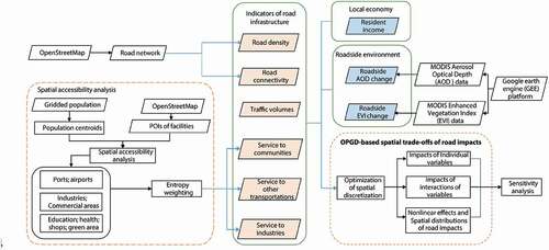
Figure 1 shows the schematic overview of methods for assessing the spatial disparities in trade-offs between road impacts on the economy and the environment. In general, the methods consist of four steps: (i) Road density and road connectivity were calculated at an LGA level; (ii) spatial accessibility analysis was performed for each category of facilities, and the road services to communities, other transportations (e.g. ports and airports), and industries were estimated as the sum entropy weighted spatial accessibilities; (iii) roadside environment conditions were defined and quantified using MODIS EVI and AOD data. The roadside environment across the whole road network was computed on GEE. Fourth, PD and PID were estimated between road transportation infrastructure variables and economic or environmental variables. The trade-offs of road impacts on the economy and environment were analyzed through the comparison of their respective PD distributions; (iv) the sensitivity of the road buffer was explored by analyzing the road impacts on the environment at four different road buffers.

Figure 1. Schematic overview of assessing spatial disparities in trade-offs between road impacts on the economy and environment

3.1. Calculation of road density and road connectivity

Road density and road connectivity are essential indicators to access road infrastructure and economic development. Road density in an LGA is a ratio between total length within the LGA and the area. Road connectivity is represented by the ratio of the number of interactions and the area. The original road network from OSM was segmented according to toad attributes, such as road name, road hierarchy, and the max speed of the road. This segmentation may lead to massive junctions located in the middle of roads, and these junctions cannot reflect the transportation capacity. To address this issue, we merged the whole road network and then identified junctions at the intersections across the network. Thus, the density of identified junctions was used to present the road connectivity within LGAs.

3.2. Accessibility analysis

Road services to communities, other transportations, and industries were evaluated using a spatial accessibility analysis. Accessibility can be characterized by the average distance from the population to the facility. In this study, a network-based accessibility analysis was used to indicate services of the three types of facilities. The method to estimate the services of facilities includes the following steps.

First, population-weighted centroids (PWCs) were computed for LGAs. Due to spatial heterogeneity of population distribution, the PWCs can more accurately reveal the clustered location of the population within a region than geometric centroids (Song et al. 2018a). The average population density between 2011 and 2016 was used to calculate PWCs using the PWC estimation method presented in Song et al. (2018a).

Second, spatial accessibility to the facility was computed using a network-based analysis method. POIs at level B were merged into level A, and all the PWCs and POIs were relocated in the road network according to the nearest Euclidean distance before the spatial accessibility. Accessibility of each category of the facility was represented by the average distance of the PWC to the nearest certain number of facilities. The numbers of target facilities were searched to determine the service capacity of facilities to local residents. If the number of targeted facilities is too small, the accessibility may be unstable and lack conviction, and if the number of target facilities is too large, the accessibility differences between different regions are blurred. A series of numbers of target destinations were set to select the suitable target destination count for different types of facilities. And the most reasonable destination counts were selected by visual checking. In this study, the number of target destinations for ports and airports and for other facilities was 2 and 10, respectively.

The final step was to present services of facilities using the sum of entropy-weighted spatial accessibility to facilities (Bao et al. 2020). Nine facility accessibilities were grouped into three categories, service to communities, service to other transportations, and service to industries using the entropy weight method. Entropy, an information indicator of variable, was used to evaluate the contribution of accessibilities for facilities in level A to the corresponding services to facilities. Thus, entropy was used to estimate the weights of accessibilities. If the information entropy of accessibility is high, a high weight should be given to the accessibility to a certain type of facility. The first step of the entropy weight method was to normalize the accessibilities. Then, the standardized value of the $j$th type of POIs at level B within the $i$th LGA is calculated as follows:

(2) $S_{ij}=\frac{P_{ij}}{{\sum }_{i=1}^n{P}_{ij}}$(2)

where $n$ is the number of LGAs, $P_{ij}$ is the normalized number $j$th POI at the $i$th LGA. Then, the information entropy $(E_j)$ and the information entropy weights $(E{W}_j)$ of the $j$th type of POI are calculated as:

(3) $E{ }_j=-\mathrm{l}\mathrm{n}{\left(n\right)}^{-1}\sum _{i=1}^n{W}_{ij}lo{g}_2{S}_{ij}$(3)

(4) $E{W}_j=\frac{1-E_j}{m-{\sum }_{j=1}^m{E}_j}$(4)

where$m$ is the number of POI types in this category. Finally, the service of roads to a category of facilities at the $i$th LGA is computed as a sum entropy weighted accessibility to facilities in this category:

(5) ${\eta }_i=\sum _{j=1}^{m}EW{ }_j\ast {\alpha }_j$(5)

where ${\alpha }_j$ is the accessibility of $j$th category of facility.

3.3. Local economy and roadside environment

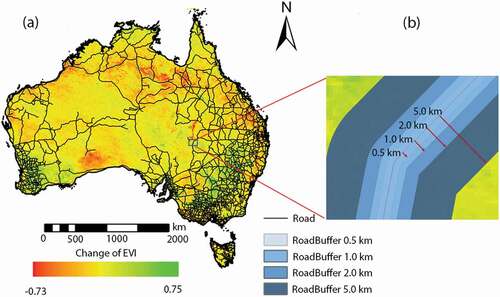
Average resident income was used to represent the local economy. The missing data at five LGAs (5/541) were filled using the inverse distance weighting (IDW) method (Donald 1968). To evaluate the roadside environment change, a 1 km buffer around the road network was generated to calculate the mean values of environmental variables within the buffer (Figure 2). Then, the roadside change of EVI and AOD of each LGA between 2016 and 2011 were calculated using the 1 km buffer from the GEE platform.

Figure 2. Road network and change of EVI derived from MODIS (a) and buffers for capturing roadside environment (e.g. EVI) (b)

3.4. OPGD-based spatial trade-offs analysis

PD and PID are used to investigate the impacts of road performance on the economy and environment. PD and PID were widely used indicators to represent the impact of explanatory variables on response variables from the perspective of spatial heterogeneity (J. F. Wang et al. 2010). PD is used to explain the impact of individual variables, and PID is used to explain the interactive impact of variables. The fundamental assumption of the indicators is that: if an explanatory variable has a significant influence on a response variable, they are probably distributed in similar spatial patterns. In this study, a strategy of the optimization of spatial discretization was used to identify optimal discretization parameters of road performance indicators (Song et al. 2020b; Song and Peng 2021). Then, the PD and PID values were calculated to represent the impacts of six road performance indicators on resident income, change of roadside EVI, and change of roadside AOD, respectively. Finally, a sensitivity analysis was performed to validate the developed methods in the study. The optimization of spatial discretization was performed using the R package “ISDA” (Song and Peng 2021) and the PD and PID values were calculated using the R package “GD” (Song et al. 2020b).

3.4.1. Optimization of spatial discretization

The geographical detector model can only deal with discrete variables to calculate the PD and PID. Thus, all continuous variables need to be converted into discrete variables before inputting the model (Wang and Chengdong 2017). The spatial data discretization method aims to divide continuous geographical and geospatial data into several intervals depending on the data’s physical or statistical characteristics (Song et al. 2020b). In this study, the optimal spatial discretization method proposed by Song and Peng (2021) was used. Firstly, all variables are divided into 3–22 groups using a quantile break. Second, for each optional parameter combination of an explanatory variable, the Q value was calculated, and a variation curve of the 75th quantile Q values was smoothed using a locally estimated scatterplot smoothing (LOESS) model. Finally, when the increase rate of the curve is lower than 5%, the point was selected as the optimal break number and used in further analysis.

Using the spatial discretization, the whole area was divided into several spatial overlay zones according to each explanatory variable. The average risk value at a zone of the explanatory variable was represented by the average value of response variables at this zone (Z. Wang et al. 2020). In this study, the spatial distribution of impacts of roads to the local economy and the roadside environment is assessed and visualized using the mean risk value.

3.4.2. Power of determinant

The PD is used to explore the explanatory power of road performance indicators on the economy and environment (Song and Peng 2021). The PD is measured by a Q value defined as:

(6) $\mathrm{Q}=1-\frac{{\sum }_{z=1}^H{N}_z{\sigma }_z^2}{N{\sigma }^2}$(6)

where $z$ is the number of spatial zones, $N_z$ and $N$ are the number of LGAs in zone $z$ and the whole study area, respectively, and ${\sigma }_z^2$ and ${\sigma }^2$ are the variance of the response variable for the units in zone $z$ and the whole study area, respectively. The Q value ranges from 0 to 1, and the Q value indicates that the explanatory variable explains 100 × Q% of the response variable. The Q value followed the noncentral F-test, which was used to determine the significance level (J. F. Wang et al. 2010)

3.4.3. Power of interactive determinant

The PID explains whether the explanatory powers of two factors are enhanced, weakened, or independent of each other (J. F. Wang et al. 2010; Hu et al. 2011; J. F. Wang, Zhang, and Fu 2016). First, the PD values of two explanatory variables $X_A$ and $X_B$ for the response variable were calculated as $Q\left(X_A\right)$ and $Q\left(X_B\right)$, respectively. Then, the PID of the interaction, a spatial overlay of factors $X_A$ and $X_B$, was calculated as $Q\left(X_A\cap X_B\right)$. The comparison between PID and individual PD indicates if variables are spatially independent, enhanced, or weakened by each other. For instance, if $Q\left(X_A\cap X_B\right)$ is higher than the sum of $Q\left(X_A\right)$ and $Q\left(X_B\right)$, the interaction of $X_A$ and $X_B$ has an enhanced effect on the response variable. Conversely, the interaction of $X_A$ and $X_B$ has a weakened effect on the response variable. If $Q\left(X_A\cap X_B\right)$ equals to $Q\left(X_A\right)+Q\left(X_B\right)$, $X_A$ and $X_B$ are spatially independent when affecting the response variable.

3.4.4. Sensitivity analysis

The sensitivity analysis was conducted to explore the influence of parameters for defining roadside environment on the road impact assessment. In the study, the roadside environment was defined as EVI and AOD values at a 1-km buffer of roads. To evaluate the impacts of the distance of buffer on the road impact assessment, the impacts were calculated and compared for roadside EVI and AOD with four different buffers around the road network in Australia (Figure 2b), including 0.5 km, 1 km, 2 km, and 5 km. The roadside change of EVI and AOD between 2011 and 2016 was evaluated within each road buffer based on the GEE platform. The PD values of road impacts on roadside environment variables at four buffers were calculated to analyze the sensitivity of the buffer distance on the impact evaluations. As a result, the variations of PD values under different distances of buffers can demonstrate the sensitivity of the methods.

4. Results

4.1. Spatial patterns

4.1.1. Local economy and roadside environment

Figure 3 shows spatial distributions and urban-rural comparisons of resident income and changes of roadside EVI and AOD. Resident income has a slight urban-rural disparity, where the urban resident income ($59,299 per year) is 15.17% higher than the rural resident income ($51,487 per year). Resident income in major cities is higher than in other regions.

Figure 3. Spatial distributions (top) and density distributions (bottom) of local economy and environment changes: (a, d) resident income; (b, e) change of roadside EVI; and (c, f) change of roadside AOD. Roadside EVI and AOD are derived from MODIS

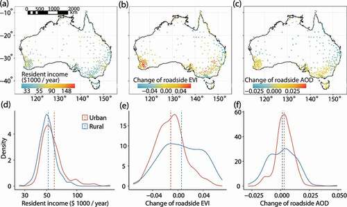
From the perspective of the environment, the change of the roadside environment from 2011 to 2016 also contains regional disparities. Vegetation plays an important role in both the regional hydrological cycle, climate regulation, and ecological sustainability. EVI can characterize vegetation cover changes very well (Duarte et al. 2018). The roadside EVI is increased in rural areas with 0.0058 EVI change, but it is decreased in urban areas with −0.0110 of EVI change. Roadside EVI decreases more in major cities than in suburban and rural areas. Suburban areas have the highest increase of EVI. The change of roadside EVI reflects the impact of human activities on the roadside environment, including infrastructure construction and road transport (Jantunen et al. 2006). The decrease of roadside EVI in urban areas reveals road transportation infrastructure has a negative impact on the environment (Ghosh, Raj, and Maiti 2020).

AOD is an indicator of atmospheric conditions in a region. The main factors contributing to the increase in AOD are polluting gases from industrial production, construction, transport, and other human activities. In Australia, AOD slightly increased in most areas, where the growth of AOD in urban areas is 2.1 times higher than that in rural areas, which was 0.0030 and 0.0014, respectively. The highest increase in AOD appears in the major cities and suburban areas. In inland areas and some parts of east areas, the AOD decreased, which indicates the improvement in air quality. In summary, from the spatial perspective, roadside environmental changes are closely linked with economic growth.

4.1.2. Road performance

Table 2 shows the weights of accessibilities to nine types of facilities in the three categories. The spatial accessibility to each of the three categories of facilities, which is used to estimate the road services to facilities, is the sum of weighted accessibilities to different types of facilities in the category.

Table 2. The entropy weights of accessibility

Accessibility to three categories of facilities	Accessibility different types of facilities in the category	Entropy weight
Communities	Residential area	0.227
	Public	0.197
	Health	0.180
	Green space and Sport area	0.224
	Education	0.172
Other transportations	Ports	0.518
	Airports	0.481
Industries	Industry	0.391
	Commercial	0.610

Figure 4 shows spatial distributions of road performance indicators. In general, road performance indicators perform better in major cities than that in suburban areas and rural areas. In major cities, services to communities and industries perform better than the service to other transportations, including ports and airports. The average distance of services to communities and industries ranges from 1.0 km to 7.4 km, while its ranges from 7.4 km to 54.6 km to other transportations.

Figure 4. Spatial distributions of road performance indicators: (a) road density, (b) road connectivity, (c) traffic volumes, (d) service to communities, (e) service to other transportations, and (f) service to industries

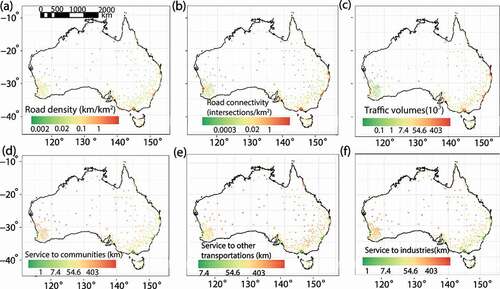
The three direct road performance indicators, road density, road connectivity, and traffic volumes, are generally correlated with regional economic development. The differences between the three indicators in major cities, suburban areas, and rural areas are significant. As for the three indirect indicators, services to facilities, in addition to being influenced by the overall level of economic development, are also related to the industrial structure of the region and the type of facilities it leads to. For example, the services to other transportations in major cities and coastal cities ranges from 7.4 km to 54.6 km, while are above 54.6 km in suburban areas. However, in most of the suburban areas, services to the industry are below 7.4 km, with less difference with major cities.

Table 3 shows a statistical summary of response variables, including economy, roadside environment, and road performance indicators. The mean LGA-based income is 55,100, USD and the coefficient of variation (CV) of resident income is 0.30. The CV values of changes of roadside EVI and AOD are −12.87 and 4.54, respectively. The CV values indicate that the changes of EVI and AOD have much higher spatial disparities than resident income. The mean road density and connectivity are 0.44 km/km² and 1.07 interactions/km². The mean traffic volume of LGAs is 16,170 per road. The mean distance between PWCs and facilities of communities, other transportations, and industries are 91.97 km, 252.23 km, and 55.39 km, respectively.

Table 3. Statistical summary of economic and roadside environmental variables and road performance indicators

	Variable	Code	Mean	Median	SD	Min	Max	CV
Response variable	Resident income ($1,000)	/	55.10	51.71	16.44	26.35	216.01	0.30
	Change of roadside EVI^※	/	−0.0023	−0.0051	0.0290	−0.0704	0.0699	−12.41
	Change of roadside AOD^※	/	0.0022	0.0027	0.0100	−0.0283	0.0490	4.54
Road performance indicators	Road density (km/km^2)	rd	0.44	0.08	0.84	0.00	5.76	1.90
	Road connectivity (interactions/km^2)	rc	1.07	0.02	2.77	0.00	22.01	2.58
	Traffic volumes (10^3)	vlm	16.17	5.17	30.16	0.02	412.55	1.87
	Service to communities (km)	sc	91.97	43.13	136.54	0.85	1107.01	1.49
	Service to other transportations (km)	st	252.23	183.02	269.30	0.00	2096.52	1.07
	Service to industries (km)	si	55.39	22.78	91.62	0.00	870.30	1.65

^※Roadside EVI and AOD are derived from MODIS.

4.2. Road impacts on economy and environment

4.2.1. Optimal spatial discretization

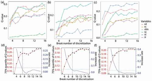
Figure 5 shows the process of optimal spatial data discretization for the analysis of resident income, change of roadside EVI, and change of roadside AOD. With the break number increased from 3 to 16, the Q values of road performance indicators are generally increased (Figure 5 a–c), but the increase rate is gradually reduced (Figure 5 d-f). When the increase rate is lower than 0.05, the optimal break number is selected (Song and Peng 2021). The optimal numbers of spatial discretization are 7, 8, and 8 for spatial analysis of resident income, the change of EVI, and the change of AOD, respectively.

Figure 5. Processes and results of the optimization of spatial discretization for resident income (a, d), change of roadside EVI (b, e), and change of roadside AOD (c, f)

4.2.2. PD and PID of roads to economy and environment

Figure 6 shows the PD and PID of road transportation infrastructure on the local economy and roadside environment. Road density and service to communities have the largest impact on resident income, with Q values of 0.2775 and 0.2754, respectively. Highly dense roads can benefit the resident income. Road service to communities has a higher impact on resident income than services to other facilities. Community facilities include schools, hospitals, and public facilities, which are most relevant to human’s daily activities. Results also show that the road service to public facilities brings more benefits to the resident income than the service to industries. Thus, the investment and construction of the living facilities are helpful for improving local resident income.

Figure 6. PD (top) and PID (bottom) of road performance indicators to resident income (a, d), change of roadside EVI (b, e), and change of roadside AOD (c, f)

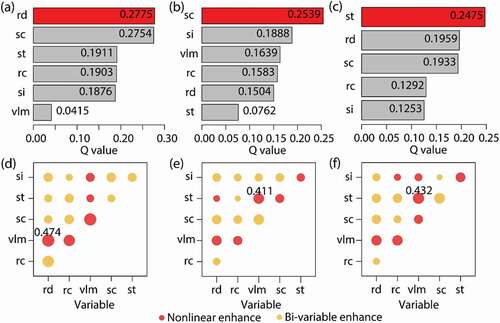
The interaction of traffic volumes with all the other variables has a nonlinear enhancing effect on resident income. Resident income is determined by multiple mixed factors, which are difficult to be measured (Glaeser, Kahn, and Rappaport 2008; Xue ting et al. 2018). This study shows that the interaction between traffic volumes and road density can explain 47.4% of resident income. The service to communities has the highest impact on the change of roadside EVI, with a Q value of 0.2539. And service to other transportations has the highest impact on the change of roadside AOD, with a Q value of 0.2475. The interaction of service to other transportations and traffic volumes has the highest impact on the roadside environment, explaining 41.1% of the change of roadside EVI and 43.2% of the change of roadside AOD. Most of the imports and exports rely on port transportation in Australia. Maritime exports in 2016 were 1,394.5 million tonnes, comprising 909.5 million tons of crude oil and inedible materials (except fuels) and 440.2 million tons of mineral fuels, lubricants, and related materials in Australia (BITRE 2018). The change of the roadside environment is mainly because of the air pollution from freight transportation between ports and industrial regions, including mining, oil and gas products, grain, and other agricultural products.

Results show the distinctive impacts of traffic volumes on the local economy and roadside environment. Traffic volumes can be regarded as the proxy of economic vitality (Li, Gao et al. 2020a), while they can only explain 4.15% of resident income and 16.39% of roadside EVI. But our result shows traffic volumes and other road infrastructure performance have an extremely nonlinear enhanced impact on the local economy and roadside environment, which can explain nearly 50% of resident income, change of roadside EVI, and change of roadside AOD. This means only enough traffic volumes or economic vitality is insufficient to promote economic growth and environmental change, but when it is integrated with well-built road infrastructure, including roads and service facilities, the economy will develop rapidly, although environmental change will also intensify. On the other side, economic development also relies on adequate social-economic vitality, including a stable investment environment and reasonable economic policies. Only well-constructed infrastructure construction is not enough.

4.2.3. Spatial distributions and trade-offs of impacts

Road density and road connectivity are direct indicators to represent road performances. Figure 7 shows the impacts of road density and road connectivity on the local economy and roadside environment, revealed by risk values from the geographical detector. The spatial disparities and nonlinearity of road impacts on the economy and environment are revealed. In major cities, road density and road connectivity have the highest impacts on resident income (refer to the red dots in the first map of Figure 7 a, b). Areas with the highest road density (range from 1.16 km/km² to 5.76 km/km²) and the highest road connectivity (range from 2.27 interactions/km² to 22 interactions/km²) have the highest resident income, which is 75,560 USD and 69,780, USD respectively. Resident income in suburban areas has the lowest dependence on road density and road connectivity.

Figure 7. Trade-offs between road impacts on income and roadside environment: regional impacts of road density (a) and connectivity (b). Different colors of dots in maps represent the positive or negative impacts on the economy and environment. Roadside EVI and AOD are derived from MODIS

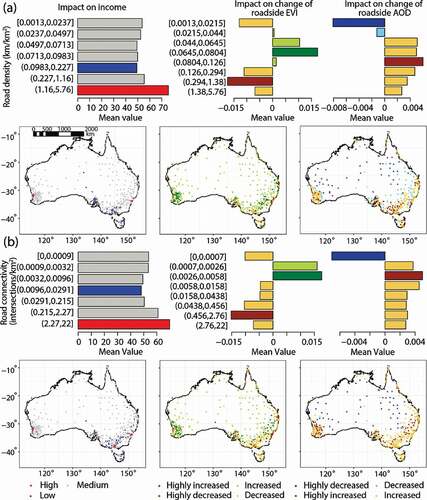
As for environmental impacts, road density and road connectivity negatively impact roadside vegetation in major cities, with the decreased EVI (refer to the orange dots in the second map of Figure 7 a, b). The highest decrease EVI (−1.7%) appears in the areas with a road density range from 0.294 km/km² to 1.38 km/km². The second highest decrease of EVI is −1.5% in areas with road connectivity range from 0.456 interactions/km² to 2.76 interactions/km². In suburban and rural areas, road performance has a positive impact on roadside vegetation, especially in suburban areas. The highest increase EVI (1.8%) appears in the areas with road connectivity range from 0.0026 interactions/km² to 0.0058 interactions/km². EVI also increase a lot (1.7%) in areas with road density range from 0.0645 km/km² to 0.0804 km/km². EVI is a remote sensing indicator of vegetation coverage and vegetation condition. Results also indicate that the effects of protecting and recovering roadside vegetation are varied across different regions. Among different regions, actions in suburban areas have the highest positive effect on roadside vegetation growth and recovery. Therefore, the spatial disparities of road impacts on roadside vegetation should be considered in practical road asset management and decision-making.

Traffic volumes and service to facilities are indirect indicators for road performance. Figure 8 shows the impacts of four indicators on the local economy and roadside environment. The findings from Figure 8 can be summarized into economic impact and environmental impact, as follows:

Figure 8. Regional impacts of traffic volumes and service to facilities. (a) Traffic volume; (b) service to communities; (c) service to other transportations; (d) service to industries. Different colors of dots in maps represent the positive or negative impacts on the economy and environment. Roadside EVI and AOD are derived from MODIS

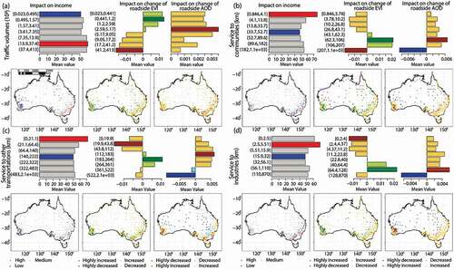
From the economic impact perspective, resident income in major cities has the highest dependence on transportation infrastructure performance (refer to the red dots in the first map of Figure 8 a-d). In suburban areas, services to facilities have relatively less importance to resident income (refer to the blue dots in the first map of Figure 8 b-d). Suburban areas with services to communities range from 33.7 km to 52.7 km have the lowest resident income ($47,485). Therefore, the investment and construction of service facilities are usually helpful for the economic growth in suburban areas. In rural areas, traffic volumes have the lowest impact on resident income (refer to the blue dots in the first map of Figure 8 a). Thus, increasing traffic volumes in rural areas is a potential approach to stimulate the local economy since traffic volumes can partially indicate local socio-economic vitality.

From the environmental impact perspective, in major cities, roads have a negative impact on roadside vegetation, as demonstrated by the decreased EVI (refer to the orange dots in the second map of Figure 8 a-d). Areas with traffic volumes range from 37,400 to 413,000 have the highest reduction in roadside EVI (−1.7%). In rural areas, traffic volumes and services to facilities are beneficial to the roadside environment, increasing roadside EVI (refer to the green dots in the second map of Figure 8 a). And the EVI in suburban areas increases more than in rural areas. Areas with service to industries range from 64.4 km to 128 km have the highest increase in roadside EVI (2.5%). Besides desert areas, all variables positively impact on the increase of roadside AOD, and traffic volumes have the highest impact. The increase of AOD in suburban areas is higher than that in major cities and rural areas.

To sum up, this study reveals the significant nonlinearity, spatial disparities, and interactions of trade-offs between road impact on the economy and the local environment. In major cities, road-related income is much higher than that in other regions. On the contrary, the local economy in suburban areas has the lowest dependence on road performance.

Major cities with the highest road-related income have higher environmental pressure than other regions, which reveals interactions of trade-offs between road impact on the local economy and the roadside environment. In suburban and rural areas, the roadside environment has improvements, with the increase of EVI. Generally, suburban areas have a higher increase of EVI than rural areas. In desert areas where environmental degradation serves, the EVI decreases a lot in the desert areas. However, road performance factors except traffic volumes can reduce the roadside AOD, which indicates that the construction of road infrastructure is beneficial to improving the desert environment.

4.3. Sensitivity analysis

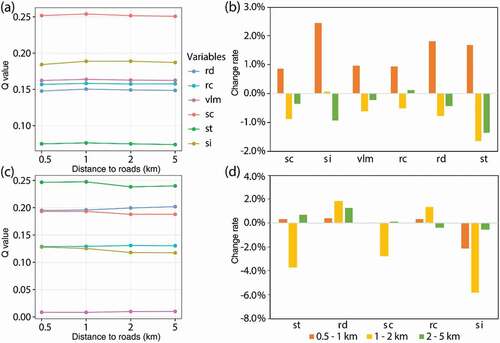
Sensitivity analysis was used to reveal the impact of the road on roadside environment change within different distances. Figure 9 shows the trend of Q values of six explanatory variables for change of roadside EVI and AOD. The order of significance of variables is not changed for all distances to roads. It shows that 1 km is the most reasonable distance to evaluate the change of roadside environment. Apart from service to industries, the road has the highest impact on EVI at 1 km for all variables. Change rates of Q values of all variables are slight, which are −1.64% to 2.44% for the change of roadside EVI and −5.81% to 1.87% for the change of roadside AOD. The road impact to the roadside EVI is most sensitive when the road buffer changes from 0.5 km to 1 km. The change rate of Q value for service to industries is 2.4%. And road impact to the roadside AOD is more sensitive from 1 km buffer to 2 km buffer, with the −1.6% change rate of Q value for service to other transportations.

Figure 9. The Q values (left) and change rates (right) of explanatory variables at different buffers for environment variables: (a, b) change of roadside EVI; (c, d) change of roadside AOD. Roadside EVI and AOD are derived from MODIS

5. Discussion

The positive impact of transportation infrastructure on resident income includes saving commuting time, connecting markets and raw materials, which can reduce transport costs, and providing job opportunities. However, road transportation infrastructure may damage the environment. The construction of road infrastructure and the erosion of soil in this process destroys the roadside vegetation and thus decrease the EVI. In addition, industrial facilities will come with an AOD increase. Therefore, the trade-offs between the economy and the environment must be considered when investing in road transportation infrastructure. However, past studies have been less likely to analyze and characterize this impact from a spatial perspective. Road performance indicators and environmental pollution indicators mostly use statistical data or data from monitoring stations. The spatial distribution of these data is sparse, and it is difficult to reveal spatial information. As a result, the spatial patterns of environmental and economic impacts of roads have not been explored comprehensively.

In this study, the relationship between transportation infrastructure, the environment, and the economy was explored using remote sensing data and a spatial heterogeneity model. And the trade-offs between road impacts on the local economy and the roadside environment were revealed. Findings are summaries as follows. First, road density, service to communities, and service to other transportations play the most important role in determining resident income, change of roadside EVI, and change of roadside AOD, respectively. The interaction of traffic volumes with other transport infrastructure variables can significantly affect the economy and the environment. In particular, the interaction of traffic volumes with road density can explain nearly 50% of the resident income.

Second, the environmental and economic impacts of transportation infrastructure have a spatial difference. Major cities are more dependent on transportation infrastructure for economic development but face greater environmental pressures than suburban and rural areas, with the decrease of roadside EVI and rapid increase of roadside AOD. On the contrary, the roadside environment has improved in suburban and rural areas, with increased EVI and a lower increase of AOD than in major cities.

Third, road transportation infrastructure has a nonlinear impact on the economy and the environment, leading to the interactions of trade-offs between road impact on the economy and the impact on the local environment. The development of road infrastructure systems can enhance economic growth, but it also brings pressure to the roadside environment. In order to improve resident income and protect the environment, regional strategies are required for achieving sustainable road infrastructure development. The actions primarily include strategic road infrastructure maintenance and management (Song et al. 2018b), nation-wide and network-level strategies for sustainable infrastructure development (Song et al. 2020b), and roadside ecological and environmental protections.

In this study, results show that the effects of actions for improving both economic growth and roadside environment in suburban and rural areas are more significant than that in major cities. The primary reason is that major cities have higher environmental pressure than suburban and rural areas. This means that much more actions are required in major cities to decrease the environmental impacts of road infrastructure than in suburban and rural areas. Finally, road impact on the vegetation is most sensitive at the distance range from 0.5 km to 1 km around the road. In comparison, road impact on the AOD is most sensitive at the distance range from 1 km to 2 km around the road.

Road transportation infrastructure also has significant impacts on the landscape dynamic. First, road infrastructure has critical impacts on vegetation dynamics. According to our study, in major cities, roadside EVI is critically reduced due to dense roads, high traffic volumes, and well-constructed service facilities. Road density and traffic volumes lead to the highest EVI decrease (−1.7%). In suburban and rural areas, the roadside environment has improvements, with the increase of EVI. And suburban areas have a higher increase of EVI than in rural areas. Second, road infrastructure also has significant impacts on the fragmentation of landscape, especially in suburban and rural areas. The construction of road infrastructure can create separation and barriers, causing fragmentation of the landscapes and populations (Jaarsma and Willems 2002). Areas with high demands of transport infrastructure have the highest fragmented landscape units (Andrea et al. 2017). To explore the environmental impact of roads, this study uses roadside EVI as the proxy of vegetation. The decrease in EVI might reveal the vegetation degradation or the increase of other land cover types. The latter reason can represent the increase of landscape fragmentation while our result can’t fully prove it. Further study can use land cover data to explore the road impact on landscape fragmentation.

Road infrastructure performance is represented by six variables in this study. Road density and road connectivity are the direct indicators that characterize road infrastructure performance. Road density reflects the length of road construction, and road connectivity demonstrates the capacity of the road (Damania et al. 2018). The interaction of the two factors with traffic volume explains nearly 50% of the resident income. In major cities, road density and connectivity have the most significant positive impact on resident income. But they threaten the roadside environment, with the decrease of roadside EVI and increase of roadside AOD. In suburban areas, the road-related income is much lower than that in major cities. And the roadside environment has improved with the increase of roadside EVI.

Traffic volumes are a good indicator of economic vitality. They interact with other road variables to provide a non-linear enhancement impact on the local economy and the roadside environment. Traffic volumes also imply the generation of vehicle emissions that can cause unavoidable AOD growth. However, traffic volumes have a positive effect on roadside vegetation in suburban and rural areas, with the max increase of EVI is 0.013.

Services to facilities reflect the service performance of road infrastructure from a socio-economic perspective. High accessibility can reduce commuting time and decreases congestion, thus reducing emissions to some extent. Therefore, services to facilities lead to EVI growth in suburban and rural areas. The highest increase of EVI (2.5%) appears in areas with services to industries range from 64.4 km to 128 km. But in major cities, services to facilities would threaten the roadside environment because of more traffic volumes associated with denser facilities compared to suburban and rural areas, leading to a large amount of exhaust gas. Besides, freight transportation to ports includes many mineral fuels, oil, gas materials, which can bring pressure to the roadside environment.

Current studies usually employed economic models or time series analysis to explore the impact of transport infrastructure on the economy and the environment, which failed to reveal the impact from the perspective of spatial (Mohmand, Wang, and Saeed 2017). Besides, enough attention has not been paid to discuss the trade-offs of the impact of the road on the economy and the environment. The main contributions of this study to road transportation research are as follows. First, road performance and roadside environmental change were evaluated by geospatial data, including POIs, population data, remote sensing data. Service to facilities was represented by accessibility using a network-based accessibility analysis method. Second, spatial trade-offs between the impact of road infrastructure on the economy and that on the roadside environment were investigated using an OPGD model. Third, the spatial difference of road impacts on the economy and the local environment was explored using mean risk values. To sum up, this study considers the heterogeneity of the spatial distribution of transport infrastructure and uses a spatial analysis model to reveal the impact of transportation infrastructure on the local economy and the environment.

There are still shortcomings in this study. First, the impact of road infrastructure performance on the economy and environment may take some time to fully manifest, but the long-time series analysis was not conducted in this study due to the limited available data. Follow-up studies should combine spatial analysis methods with a time analysis model to make a deeper analysis of the mechanism of the impact of transport infrastructure on the economy and the environment. In addition, spatial autocorrelation was not considered when conducting a spatial analysis model. Future studies should use a spatial model that combines spatial heterogeneity and spatial autocorrelation to better explain the impact of roads on the environment and economy.

6. Conclusion

This study investigates the impacts of road transportation infrastructure on the local economy and roadside environment using spatial heterogeneity methods. The spatial disparities in trade-offs have been assessed between road impacts on the economy and environment. Significant nonlinearity and spatial disparities, such as urban-rural variations, have been identified in the trade-offs. In general, roadside EVI is decreased, and roadside AOD is critically increased in major cities together with economic growth. However, in suburban and rural areas, roadside EVI is increased, and the increase of roadside AOD is much lower than that in major cities, although the economic development is approximate with that in major cities. Therefore, this study reveals that the environmental pressure from road transportation in major cities is much higher than that in suburban and rural areas. Results show that the effects of actions for improving both economic growth and roadside environment in suburban and rural areas are more significant than that in major cities. The primary reason is that major cities have higher environmental pressure than suburban and rural areas. This means that much more actions are required in major cities to decrease the environmental impacts of road infrastructure than in suburban and rural areas. This study contributes to a deep understanding of the interaction between road infrastructure, economy, and environment and can also guide the authorities to make strategic decisions for sustainable infrastructure development.

Abbreviations

The following abbreviations are used in this manuscript:

AOD: Aerosol Optical Depth

EVI: Enhanced Vegetation Index

NDVI: Normalized Difference Vegetation Index

PD: Power of determinants

PID: Power of interactive determinants

POI: Point of interests

OPGD: Optimal parameters-based geographical detector

LGA: Local Government Area

PWC: Population-weighted centroids

rc: Road density

rc: Road connectivity

vlm: Traffic volumes

sc: Service to communities

si: Service to industries

st: Service to other transportations

Acknowledgements

This research was supported by the Australian Government through the Australian Research Council’s Discovery Early Career Researcher Award funding scheme (Project No. DE170101502), and Discovery Project (Project No. DP180104026).

Disclosure statement

No potential conflict of interest was reported by the author(s).

Additional information

Funding

This work was supported by the Australian Research Council [DE170101502; DP180104026].

References

- ABS (Australian Bureau of Statitics). 2015. Australian Transport Economic Account : An Experimental Transport Satellite Account. Catalogue Number 5270.0. https://www.abs.gov.au/statistics/economy/national-accounts/australian-transport-economic-account-experimental-transport-satellite-account/latest-release
- ABS (Australian Bureau of Statitics). 2020. Personal Income in Australia. Catalogue Number 6524.0.55.022. https://www.abs.gov.au/statistics/labour/earnings-and-work-hours/personal-income-australia/2011-12-2017-18
- Agbelie, B. R. D. K. 2014. “An Empirical Analysis of Three Econometric Frameworks for Evaluating Economic Impacts of Transportation Infrastructure Expenditures across Countries.” Transport Policy 35: 304–310. Elsevier. doi:10.1016/j.tranpol.2014.06.009.
- Allen, C., G. Metternicht, T. Wiedmann, and M. Pedercini. 2019. “Greater Gains for Australia by Tackling All SDGs but the Last Steps Will Be the Most Challenging.” Nature Sustainability 2 (11): 1041–1050. doi:10.1038/s41893-019-0409-9. Springer US.
- Allen, C., M. Reid, J. Thwaites, R. Glover, and T. Kestin. 2020. “Assessing National Progress and Priorities for the Sustainable Development Goals (Sdgs): Experience from Australia.” Sustainability Science 15 (2): 521–538. doi:10.1007/s11625-019-00711-x.
- Allen, C. D., R. Ferrare, J. Szykman, J. Lewis, A. Scarino, J. Hains, and S. Burton. 2015. “Regional Characteristics of the Relationship between Columnar AOD and Surface PM2.5: Application of Lidar Aerosol Extinction Profiles over Baltimore-Washington Corridor during DISCOVER-AQ.” Atmospheric Environment 101: 338e349. Elsevier Ltd. doi:10.1016/j.atmosenv.2014.11.034.
- Allen, T., and C. Arkolakis. 2020. “The Welfare Effects of Transportation Infrastructure Improvements.” Journal of Chemical Information and Modeling 01 (01): 1689–1699.
- Alvarez-Mendoza, C. I., A. Teodoro, and L. Ramirez-Cando. 2019. “Spatial Estimation of Surface Ozone Concentrations in Quito Ecuador with Remote Sensing Data, Air Pollution Measurements and Meteorological Variables.” Environmental Monitoring and Assessment 191(3). Environmental Monitoring and Assessment. doi:10.1007/s10661-019-7286-6.
- Al-Yaari, A., J. P. Wigneron, W. Dorigo, A. Colliander, T. Pellarin, S. Hahn, and A. Mialon. 2019. “Assessment and Inter-Comparison of Recently Developed/Reprocessed Microwave Satellite Soil Moisture Products Using ISMN Ground-Based Measurements.” Remote Sensing of Environment 224 (February): 289–303. doi:10.1016/j.rse.2019.02.008. Elsevier.
- Anderson, K., B. Ryan, W. Sonntag, A. Kavvada, and L. Friedl. 2017. “Earth Observation in Service of the 2030 Agenda for Sustainable Development.” Geo-Spatial Information Science 20 (2): 77–96. doi:10.1080/10095020.2017.1333230. Taylor & Francis.
- Andrea, D. M., B. Martín, E. Ortega, A. Ledda, and V. Serra. 2017. “Landscape Fragmentation in Mediterranean Europe: A Comparative Approach.” Land Use Policy 64: 83–94. Elsevier Ltd. doi:10.1016/j.landusepol.2017.02.028.
- Bao, Q., Z. Yuxin, W. Yuxiao, and Y. Feng. 2020. “Can Entropy Weight Method Correctly Reflect the Distinction of Water Quality Indices?.” Water Resources Management 34 (11): 3667–3674. doi:10.1007/s11269-020-02641-1. Water Resources Management.
- Bishop-Taylor, R., M. G. Tulbure, and M. Broich. 2018. “Evaluating Static and Dynamic Landscape Connectivity Modelling Using a 25-Year Remote Sensing Time Series.” Landscape Ecology 33 (4): 625–640. doi:10.1007/s10980-018-0624-1. Springer Netherlands.
- BITRE. 2018. Australian Sea Freight 2015–16. https://www.bitre.gov.au/publications/2018/asf_2015_16.aspx.
- Boulila, W., I. R. Farah, and A. Hussain. 2018. “A Novel Decision Support System for the Interpretation of Remote Sensing Big Data.” Earth Science Informatics 11 (1): 31–45. doi:10.1007/s12145-017-0313-7. Earth Science Informatics.
- Cai, J., B. Xu, K. Kie Yan Chan, X. Zhang, B. Zhang, Z. Chen, and B. Xu. 2019. “Roles of Different Transport Modes in the Spatial Spread of the 2009 Influenza A(H1N1) Pandemic in Mainland China.” International Journal of Environmental Research and Public Health 16(2). MDPI AG. doi:10.3390/ijerph16020222.
- Cârlan, I., D. Haase, A. Große-Stoltenberg, and I. Sandric. 2020. “Mapping Heat and Traffic Stress of Urban Park Vegetation Based on Satellite Imagery - A Comparison of Bucharest, Romania and Leipzig, Germany.” Urban Ecosystems 23 (2): 363–377. doi:10.1007/s11252-019-00916-z. Urban Ecosystems.
- Cochran, F., J. Daniel, L. Jackson, and A. Neale. 2020. “Earth Observation-Based Ecosystem Services Indicators for National and Subnational Reporting of the Sustainable Development Goals.” Remote Sensing of Environment 244 (February): 111796. doi:10.1016/j.rse.2020.111796. Elsevier.
- Damania, R., J. Russ, D. Wheeler, and A. F. Barra. 2018. “The Road to Growth: Measuring the Tradeoffs between Economic Growth and Ecological Destruction.” World Development 101 (August): 351–376. doi:10.1016/j.worlddev.2017.06.001.
- Daniel(Jian), S., Z. Kaisheng, and S. Suwan. 2018. “Analyzing Spatiotemporal Traffic Line Source Emissions Based on Massive Didi Online Car-Hailing Service Data.” Transportation Research Part D: Transport and Environment 62 (800): 699–714. doi:10.1016/j.trd.2018.04.024.
- Deljouei, A., S. Seyed Mohammad Moein, E. Abdi, M. Bernhardt-Römermann, E. L. Pascoe, and M. Marcantonio. 2018. “The Impact of Road Disturbance on Vegetation and Soil Properties in a Beech Stand, Hyrcanian Forest.” European Journal of Forest Research 137 (6): 759–770. doi:10.1007/s10342-018-1138-8. Springer Berlin Heidelberg.
- Didan, K., A. B. Munoz, R. Solano, and A. Huete. 2015. “MODIS Vegetation Index User ’S Guide (Collection 6).” 2015 (May): 31.
- Ding, Y., M. Zhang, X. Qian, L. Chengren, S. Chen, and W. Wang. 2019. “Using the Geographical Detector Technique to Explore the Impact of Socioeconomic Factors on PM2.5 Concentrations in China.” Journal of Cleaner Production 211: 1480–1490. Elsevier Ltd. doi:10.1016/j.jclepro.2018.11.159.
- Donald, S. 1968. “Two- Dimensional Interpolation Function for Irregularly- Spaced Data.” Proc 23rd Nat Conf, New York, 517–524.
- Du, Z., X. Xiaoming, H. Zhang, W. Zhitao, and Y. Liu. 2016. “Geographical Detector-Based Identification of the Impact of Major Determinants on Aeolian Desertification Risk.” PLoS ONE 11(6). Public Library of Science. doi:10.1371/journal.pone.0151331.
- Duarte, L., A. C. Teodoro, A. T. Monteiro, M. Cunha, and G. Hernâni. 2018. “QPhenoMetrics: An Open Source Software Application to Assess Vegetation Phenology Metrics.” Computers and Electronics in Agriculture 148 (October 2017): 82–94. doi:10.1016/j.compag.2018.03.007. Elsevier.
- Erjia, G., R. Zhang, D. Li, X. Wei, X. Wang, and P. C. Lai. 2017. “Estimating Risks of Inapparent Avian Exposure for Human Infection: Avian Influenza Virus A (H7N9) in Zhejiang Province, China.” Scientific Reports 7(January). Nature Publishing Group. doi:10.1038/srep40016.
- Gaughan, A. E., F. R. Stevens, C. Linard, P. Jia, and A. J. Tatem. 2013. “High Resolution Population Distribution Maps for Southeast Asia in 2010 and 2015.” PLoS ONE 8 (2). doi:10.1371/journal.pone.0055882.
- Ge, Y. J., A. Thomasson, and R. Sui. 2011. “Remote Sensing of Soil Properties in Precision Agriculture: A Review.” Frontiers of Earth Science 5 (3): 229–238. doi:10.1007/s11707-011-0175-0.
- Ghosh, S. P., D. Raj, and S. K. Maiti. 2020. “Risks Assessment of Heavy Metal Pollution in Roadside Soil and Vegetation of National Highway Crossing through Industrial Area.” Environmental Processes 7 (4): 1197–1220. doi:10.1007/s40710-020-00463-2. Environmental Processes.
- Glaeser, E. L., M. E. Kahn, and J. Rappaport. 2008. “Why Do the Poor Live in Cities? the Role of Public Transportation.” Journal of Urban Economics 63 (1): 1–24. doi:10.1016/j.jue.2006.12.004.
- Haklay, M., and P. Weber. 2008. “Openstreetmap: User-Generated Street Maps.” IEEE Pervasive Computing 7 (4): 12–18. doi:10.1109/MPRV.2008.80.
- Hall, N. L., S. Creamer, W. Anders, A. Slatyer, and P. S. Hill. 2020. “Water and Health Interlinkages of the Sustainable Development Goals in Remote Indigenous Australia.” Npj Clean Water 3(4). Springer US. doi:10.1038/s41545-020-0060-z.
- Hu, Y., J. Wang, L. Xiaohong, D. Ren, and J. Zhu. 2011. “Geographical Detector-Based Risk Assessment of the under-Five Mortality in the 2008 Wenchuan Earthquake, China.” PLoS ONE 6 (6). doi:10.1371/journal.pone.0021427.
- Im, J. 2020. “Earth Observations and Geographic Information Science for Sustainable Development Goals.” GIScience and Remote Sensing 57 (5): 591–592. doi:10.1080/15481603.2020.1763041. Taylor & Francis.
- Jaarsma, C. F., and G. P. A. Willems. 2002. “Reducing Habitat Fragmentation by Minor Rural Roads through Traffic Calming.” Landscape and Urban Planning 58 (2–4): 125–135. doi:10.1016/S0169-2046(01)00215-8.
- Jantunen, J., K. Saarinen, A. Valtonen, and S. Saarnio. 2006. “Grassland Vegetation along Roads Differing in Size and Traffic Density.” Annales Botanici Fennici 43 (2): 107–117.
- Karagulian, F., C. A. Belis, C. F. C. Dora, A. M. Prüss-Ustün, S. Bonjour, H. Adair-Rohani, and M. Amann. 2015. “Contributions to Cities’ Ambient Particulate Matter (PM): A Systematic Review of Local Source Contributions at Global Level.” Atmospheric Environment 120: 475–483. Elsevier Ltd. doi:10.1016/j.atmosenv.2015.08.087.
- Khan, R., U. Haroon, M. Siddique, K. Zaman, S. U. Yousaf, A. M. Shoukry, S. Gani, A. K. Sasmoko, S. S. Hishan, and H. Saleem. 2018. “The Impact of Air Transportation, Railways Transportation, and Port Container Traffic on Energy Demand, Customs Duty, and Economic Growth: Evidence from a Panel of Low-, Middle-, and High -income Countries.” Journal of Air Transport Management 70 (February 2017): 18–35. doi:10.1016/j.jairtraman.2018.04.013. Elsevier Ltd.
- Li, B., S. Gao, Y. Liang, Y. Kang, T. Prestby, Y. Gao, and R. Xiao. 2020a. “Estimation of Regional Economic Development Indicator from Transportation Network Analytics.” Scientific Reports 10 (1): 1–15. doi:10.1038/s41598-020-59505-2. Springer US.
- Li, D., and Y. Liao. 2018. “Spatial Characteristics of Heavy Metals in Street Dust of Coal Railway Transportation Hubs: A Case Study in Yuanping, China.” International Journal of Environmental Research and Public Health 15 (12). doi:10.3390/ijerph15122662.
- Li, S., D. Lyu, G. Huang, X. Zhang, F. Gao, Y. Chen, and X. Liu. 2020b. “Spatially Varying Impacts of Built Environment Factors on Rail Transit Ridership at Station Level: A Case Study in Guangzhou, China.” Journal of Transport Geography 82 (July 2019). doi:10.1016/j.jtrangeo.2019.102631.
- Liao, Y., J. Wang, D. Wei, B. Gao, X. Liu, G. Chen, X. Song, and X. Zheng. 2017. “Using Spatial Analysis to Understand the Spatial Heterogeneity of Disability Employment in China.” Transactions in GIS 21 (4): 647–660. doi:10.1111/tgis.12217. Blackwell Publishing Ltd.
- Ma, H., J. Zeng, N. Chen, X. Zhang, M. H. Cosh, and W. Wang. 2019. “Satellite Surface Soil Moisture from SMAP, SMOS, AMSR2 and ESA CCI: A Comprehensive Assessment Using Global Ground-Based Observations.” Remote Sensing of Environment 231 (February): 111215. doi:10.1016/j.rse.2019.111215. Elsevier.
- Mann, D., G. Agrawal, and P. K. Joshi. 2019. “Spatio-Temporal Forest Cover Dynamics along Road Networks in the Central Himalaya.” Ecological Engineering 127 (November 2018): 383–393. doi:10.1016/j.ecoleng.2018.12.020. Elsevier.
- Martins, V. S., A. Lyapustin, Y. Wang, D. M. Giles, A. Smirnov, I. Slutsker, and S. Korkin. 2019. “Global Validation of Columnar Water Vapor Derived from EOS MODIS-MAIAC Algorithm against the Ground-Based AERONET Observations.” Atmospheric Research 225 (April): 181–192. doi:10.1016/j.atmosres.2019.04.005. Elsevier.
- Matsushita, B., W. Yang, J. Chen, Y. Onda, and G. Qiu. 2007. “Sensitivity of the Enhanced Vegetation Index (EVI) and Normalized Difference Vegetation Index (NDVI) to Topographic Effects: A Case Study in High-Density Cypress Forest.” Sensors 7 (11): 2636–2651. doi:10.3390/s7112636.
- Mohmand, Y. T., A. Wang, and A. Saeed. 2017. “The Impact of Transportation Infrastructure on Economic Growth: Empirical Evidence from Pakistan.” Transportation Letters 9 (2): 63–69. doi:10.1080/19427867.2016.1165463.
- Pathak, C., S. Chandra, G. Maurya, A. Rathore, M. O. Sarif, and R. D. Gupta. 2021. “The Effects of Land Indices on Thermal State in Surface Urban Heat Island Formation: A Case Study on Agra City in India Using Remote Sensing Data (1992–2019).” Earth Systems and Environment 5 (1): 135–154. doi:10.1007/s41748-020-00172-8. Springer International Publishing.
- Schultz, M., J. Voss, M. Auer, S. Carter, and A. Zipf. 2017. “Open Land Cover from OpenStreetMap and Remote Sensing.” International Journal of Applied Earth Observation and Geoinformation 63 (May): 206–213. doi:10.1016/j.jag.2017.07.014. Elsevier.
- Shi, H., T. Shi, Z. Yang, Z. Wang, F. Han, and C. Wang. 2018. “Effect of Roads on Ecological Corridors Used for Wildlife Movement in a Natural Heritage Site.” Sustainability (Switzerland) 10 (8): 1–24. doi:10.3390/su10082725.
- Shrestha, A., and W. Luo. 2017. “An Assessment of Groundwater Contamination in Central Valley Aquifer, California Using Geodetector Method.” Annals of GIS (3). . doi:10.1080/19475683.2017.1346707. Taylor and Francis Ltd
- Song, Y., Y. Tan, Y. Song, P. Wu, J. C. P. Cheng, M. J. Kim, and X. Wang. 2018a. “Spatial and Temporal Variations of Spatial Population Accessibility to Public Hospitals: A Case Study of Rural–Urban Comparison.” GIScience and Remote Sensing 55 (5): 718–744. doi:10.1080/15481603.2018.1446713. Springer US
- Song, Y., G. L. Wright, P. Wu, D. Thatcher, T. McHugh, Q. Li, S. J. Li, and X. Wang. 2018b. “Segment-Based Spatial Analysis for Assessing Road Infrastructure Performance Using Monitoring Observations and Remote Sensing Data.” Remote Sensing 10 (11). doi:10.3390/rs10111696
- Song, Y., P. Wu, D. Gilmore, and Q. Li. 2020a. “A Spatial Heterogeneity-Based Segmentation Model for Analyzing Road Deterioration Network Data in Multi-Scale Infrastructure Systems.” IEEE Transactions on Intelligent Transportation Systems 1–11. doi:10.1109/tits.2020.3001193
- Song, Y., J. Wang, Y. Ge, and C. Xu. 2020b. “An Optimal Parameters-Based Geographical Detector Model Enhances Geographic Characteristics of Explanatory Variables for Spatial Heterogeneity Analysis: Cases with Different Types of Spatial Data.” GIScience and Remote Sensing 57 (5): 593–610. doi:10.1080/15481603.2020.1760434. Taylor & Francis
- Song, Y., and P. Wu. 2021. “An Interactive Detector for Spatial Associations.” International Journal of Geographical Information Science. doi:10.1080/13658816.2021.1882680
- Stevens, F. R., A. E. Gaughan, C. Linard, and A. J. Tatem. 2015a. “Disaggregating Census Data for Population Mapping Using Random Forests with Remotely-Sensed and Ancillary Data.” PLoS ONE 10 (2): 1–22. doi:10.1371/journal.pone.0107042.
- Umar, M., J. Xiangfeng, D. Kirikkaleli, and X. Qinghui. 2020. “COP21 Roadmap: Do Innovation, Financial Development, and Transportation Infrastructure Matter for Environmental Sustainability in China?.” Journal of Environmental Management 271 (June): 111026. doi:10.1016/j.jenvman.2020.111026. Elsevier Ltd.
- Viana, J., J. V. Santos, R. M. Neiva, J. Souza, L. Duarte, A. C. Teodoro, and A. Freitas. 2017. “Remote Sensing in Human Health: A 10-Year Bibliometric Analysis.” Remote Sensing 9 (12): 1–12. doi:10.3390/rs9121225.
- Wang, J., and X. Chengdong. 2017. “Geodetector: Principle and Prospective.” Acta Geographica Sinica 72 (1): 116–134. doi:10.11821/dlxb201701010. Science Press.
- Wang, J. F., T. L. Zhang, and B. J. Fu. 2016. “A Measure of Spatial Stratified Heterogeneity.” Ecological Indicators 67: 250–256. Elsevier Ltd. doi:10.1016/j.ecolind.2016.02.052.
- Wang, J. F., X. H. Li, G. Christakos, Y. L. Liao, T. Zhang, G. Xue, and X. Y. Zheng. 2010. “Geographical Detectors-Based Health Risk Assessment and Its Application in the Neural Tube Defects Study of the Heshun Region, China.” International Journal of Geographical Information Science 24 (1): 107–127. doi:10.1080/13658810802443457.
- Wang, L., and L. Chen. 2018. “Analysis: The Impact of New Transportation Modes on Population Distribution in Jing-Jin-Ji Region of China.” Scientific Data 5 (1): 1–15. doi:10.1038/sdata.2017.204. The Author(s).
- Wang, S., Y. Dexin, M. Xiaogang, and X. Xing. 2018. “Analyzing Urban Traffic Demand Distribution and the Correlation between Traffic Flow and the Built Environment Based on Detector Data and POIs.” European Transport Research Review 10 (2). doi:10.1186/s12544-018-0325-5.
- Wang, Z., C. Fan, Q. Zhao, and S. W. Myint. 2020. “A Geographically Weighted Regression Approach to Understanding Urbanization Impacts on Urban Warming and Cooling: A Case Study of Las Vegas.” Remote Sensing 12(2). MDPI AG. doi:10.3390/rs12020222.
- Xue ting, Y., Y. P. Fang, Q. Xiao ping, and F. B. Zhu. 2018. “Gradient Effect of Road Transportation on Economic Development in Different Geomorphic Regions.” Journal of Mountain Science 15 (1): 181–197. doi:10.1007/s11629-017-4498-5.
- Yang, J., P. Gong, F. Rong, M. Zhang, J. Chen, S. Liang, X. Bing, J. Shi, and R. Dickinson. 2013. “The Role of Satellite Remote Sensing in Climate Change Studies.” Nature Climate Change 3 (10): 875–883. doi:10.1038/nclimate1908.
- Yang, R., X. Qian, and H. Long. 2016. “Spatial Distribution Characteristics and Optimized Reconstruction Analysis of China’s Rural Settlements during the Process of Rapid Urbanization.” Journal of Rural Studies 47: 413–424. Elsevier Ltd. doi:10.1016/j.jrurstud.2016.05.013.
- Zhang, X., J. Nie, C. Cheng, X. Chengdong, L. Zhou, S. Shen, and Y. Pei. 2020. “Natural and Socioeconomic Factors and Their Interactive Effects on House Collapse Caused by Typhoon Mangkhut.” International Journal of Disaster Risk Science. Beijing Normal University Press. doi:10.1007/s13753-020-00322-6.
- Zhang, Y., H. Lu, and W. Qu. 2020. “Geographical Detection of Traffic Accidents Spatial Stratified Heterogeneity and Influence Factors.” International Journal of Environmental Research and Public Health 17(2). MDPI AG. doi:10.3390/ijerph17020572.
- Zhu, L., J. Meng, and L. Zhu. 2020. “Applying Geodetector to Disentangle the Contributions of Natural and Anthropogenic Factors to NDVI Variations in the Middle Reaches of the Heihe River Basin.” Ecological Indicators 117 (January): 106545. doi:10.1016/j.ecolind.2020.106545. Elsevier.