Assessment of plant species distribution and diversity along a climatic gradient from Mediterranean woodlands to semi-arid shrublands

ABSTRACT

Climate and land-use change profoundly affect plant species distribution (SD) and composition, and the impact of these processes is expected to increase in the coming years. As a proxy of global changes, knowledge of SD and diversity along climatic gradients is essential to determine the efforts needed for species conservation. Plant spectral diversity is an emerging approach used as a proxy for species diversity based on remote sensing. Thus, the research aim was to develop a comprehensive methodology based on spectral diversity for SD and richness mapping and to study their relations with environmental and human-derived factors, demonstrated along Mediterranean to semi-arid climatic gradient. The study addresses two main knowledge gaps regarding spectral diversity: (1) improving the accuracy of woody species classification by features extraction and selection, and by using texture analysis in an ecosystem characterized by high spatial variability and relatively small-sized and sparse woody vegetation; and (2) developing a better estimate of the local species ‎richness and their response to environmental and human-derived factors (i.e. climate, topography, substrate, and land cover factors) across a transition zone between Mediterranean woodlands and semi-arid dwarf shrublands. A hyperspectral image was acquired for a 43-km strip along the study area using an airborne flight of AISA-FENIX (380–2500 nm, 420 bands) at the end of the 2017 rainy season. The dominant species were surveyed, with a total number of 247 trees and shrubs, to train a machine learning support vector machine (SVM) classification for species distribution mapping, which yielded an overall accuracy of 86.1%. A feature extraction and selection methodology was developed, combining principal component analysis and neighborhood component analysis techniques, facilitating the identification of 33 spectral diagnostic bands out of 330 spectral bands. The classification accuracy was decreased by about 2% to 84.2% using only 33 spectral bands. The classification accuracy improved by about 7.1% for the seven large crown species (93.3%) by adding texture information. Later, the local species richness was calculated by utilizing the alpha diversity index (i.e. the Shannon Index) for 30-m grid cells and was tested in response to environmental (i.e. climate, substrate, and topography) and human-derived factors (i.e. land cover). The highest sensitivity to alpha diversity factors was mean annual precipitation, slope, and land surface temperature. The alpha diversity showed higher richness in the natural Mediterranean shrubland and the guarrigue located in the northern part of the climate gradient. We suggest that the approach presented here significantly improves the estimation of woody species distribution and diversity in areas characterized by high spatial heterogeneity along steep climatic gradients.

KEYWORDS:

• AISA-FENIX
• climatic gradient
• texture analysis
• species distribution
• spectral feature selection
• support vector machines
• alpha diversity

1. Introduction

Climate and land-use changes are expected to affect plant community structure, function, and composition, potentially resulting in species extinction and a decline in biodiversity (Matesanz and Valladares 2014; Barredo et al. 2016). Mediterranean ecosystems are considered “biodiversity hotspots” due to their high plant species diversity, but also “hotspots” of atmospheric warming and massive urbanization (Myers et al. 2000; Mittermeier et al. 2011). Desert-fringe Mediterranean regions are characterized by climatic gradients that reflect transitions from humid or sub-humid to dry and hot climates. Under current and future climate change rates, these transition zones have attracted significant attention as tools for understanding expected ecological changes through “Space and Time” reasoning (Roitberg et al. 2016; Roitberg and Shoshany, 2017). Biodiversity assessments are critical for revealing changes in habitat conditions and ecosystem functioning due to anthropogenic or natural processes taking place in Mediterranean regions. One of the most widely adopted approaches for assessing patterns and processes of biodiversity is ‎species diversity at both biogeography and ecological scales (Chiarucci et al., 2017). Consequently, it is instrumental for monitoring and characterizing climate-driven ecological changes along climatic gradients. Considerable research has been devoted to assessing SD change along environmental gradients in general and climatic gradients in particular (Whittaker, et al. 2001; Harrison et al. 2020). Species diversity relationships with temperature and precipitation, along climatic gradients, have been extensively studied in many areas, such as South Africa (O’Brien 1993; O’Brien, et al. 2000), grazing lands in northeastern Spain (De Bello, et al. 2006), West African countries bounding the Sahel (Da et al. 2018), Salicaceae habitats in China (Li et al. 2019), a climate gradient in Spain (Baudena et al. 2015), and the Siskiyou Mountains in Oregon (USA) (Spasojevic et al. 2014).

Field SD data gathering methods are time-consuming and highly affected by sampling design. Satellite remote sensing is considered adequate for SD mapping and monitoring (Rocchini et al. 2016; He et al. 2015), but these tools are limited in their spatial and spectral resolution (Gillespie et al. 2008). One of the leading approaches is based on the Spectral Variation Hypothesis (SVH) (Palmer et al. 2002), where spectral diversity serves as a proxy for species diversity (Wang and Gamon 2019). This approach has been utilized through different univariate and multivariate regression techniques, spectral data analysis, vegetation indices, and principal component analyses (Rocchini, et al. 2015). However, it is essential to note that most application areas of SVH are characterized by high vegetation covers, such as tropical forests, wetlands, and boreal forests (Féret and Asner 2011; Baldeck and Asner 2013). In contrast, the Mediterranean to arid climatic transition zones is characterized by high spatial variability of plants, dry organic matter, and rock exposures, which hamper species diversity mapping and monitoring. High-spatial resolution hyperspectral imaging (i.e. imaging spectroscopy (IS)) is an adequate source for SD information for such environments (Wang and Gamon 2019; Laliberté et al. 2020). IS includes hundreds of narrow contiguous spectral bands throughout the visible (VIS), near-infrared (NIR), and shortwave-infrared (SWIR) spectral regions, ranging from 400 to 2500 nm, which provides accurate and valuable spectral information on plant conditions (Goetz et al. 1985; Gillespie et al. 2008; Pena and Altmann 2009). Specific absorption features can capture leaf or canopy chemistry, enabling species identification (Ustin 2013; Asner et al. 2017). In general, plant spectral signals depend on photosynthetic pigment concentration in the VIS region, leaf structure in the NIR spectral regions, and canopy water content, lignin, cellulose, and non-structural carbohydrates in the SWIR spectral regions (Rosso, et al. 2005; Van der Meer and De Jong 2011). The “spectral diversity” concept, which uses spectral signatures and functional traits to represent regional diversity, was suggested by Féret and Asner (2014) and has been used to collect hundreds of target species in Africa and North America areas characterized by high vegetation cover. Identifying species at the individual level, along the typical Mediterranean to arid gradient, utilizing airborne IS, is a challenging task that has not yet been fully accomplished. The challenge is mainly related to the small-sized and sparse woody vegetation ranging from trees and shrubs of several meters to dwarf-shrub with a size ‎of less than 1 m. Variation in leaf area index, leaf age, leaf density, leaf orientation, stress conditions, and soil background effects could impede the search for spectral uniqueness, resulting in spectral confusion between species in Mediterranean regions.

In response to these knowledge gaps, the research aimed to develop a comprehensive approach based on spectral diversity for SD and richness mapping and study their relations with environmental and human-derived factors, demonstrated along the Mediterranean to semi-arid climatic gradient. We acquired aAISA- FENIX hyperspectral image over the climatic gradient between Mediterranean to semi-arid zones in central Israel to advance this aim. We then conducted a detailed field survey of individual trees and shrubs within the AISA-FENIX strip. Improvements in species identification were tested here by assessing different spectral band combinations and incorporating them within canopy texture parameterizations. By utilizing the comprehensive spectral and textural technique, we mapped SD along the flight line and assessed alpha diversity characteristics for different environmental factors (e.g. topography, lithology, and substrate) and human-derived factors (e.g. land-cover types).

2. Study area and data collection

2.1 Study area

The study area extends along a climatic gradient in southeastern Israel, representing a typical Mediterranean climate of mild, rainy winters and long, warm, dry summers. The growing season is usually commencing in October–November and ending in April–May. The increasing length of the season is determined by rainfall, with shorter rainy seasons in the southern area. The mean annual rainfall in the study area ranges from 500 mm in the north to around 200 mm in the south (Figure 1a). The dominant species in the areas with annual precipitation exceeding 350 mm are Quercus calliprinos, Pistacia lentiscus, Ceratonia silliqua, and Rhamnus palaestinus (Naveh and Whittaker 1980). In the desert-fringe, where mean annual rainfall is about 200 mm, the most common species are dwarf shrub species, such as Sarcopoterium spinosum and Thymelaea hirsuta (Sternberg and Shoshany 2001), with Sarcopoterium spinosum also found in vast grazing areas and areas of abandoned agriculture in Sardinia, southern Italy, Greece, Crete, Turkey, Lebanon, and North African countries (Shmida and Whittaker 1984; Tsiourlis, et al. 2007; Seligman and Zalmen 2003; Mohammad and Alseekh 2013; Evenari, et al. 1985). The human disturbance caused by grazing, woodcutting, fires, and urbanization threatens biodiversity preservation in this region. In addition, a large portion of the study site was afforested by the Forest Service of the Jewish National Fund (JNF), mainly with Pinus halepensis plantations. Therefore, the area is highly spatially heterogeneous due to the combined effects of high climatic variability, edaphic conditions, and long-term human interventions. In the past decades, this area attracted several studies concerning the impact of climate change on species diversity (Danin, et al.  1975), the effect of altitude on plant diversity (Kutiel, et al.  2000; Rysavy et al. 2014), and biomass distribution between semi-arid and desert-fringe sites (Sternberg and Shoshany 2001; Chang and Shoshany 2017; Chang, et al.  2018).

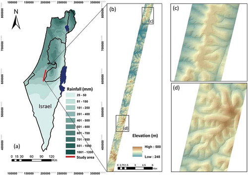
Figure 1. (a) The hyperspectral flight-line area overlaying the map of Israel with mean annual precipitation (mm/year) isohyets; (b) elevation throughout the flight line zooming into the northern (c), and southern (d) parts of the strip based on a digital elevation model (DEM) acquired from NASA’s Alaska Satellite Facility (ASF) (12.5-m resolution)

2.2. Data acquisition

2.2.1 Hyperspectral data acquisition and pre-processing

Data acquired for this study include a 43-km-long hyperspectral strip with 420 spectral wavelength bands in the VIS-NIR-SWIR (380–2500 nm) obtained by an AISA-FENIX airborne image spectrometer on 4 April 2017. The image was acquired at the end of the rainy season in a year with record low precipitation. The flight altitude was approximately 1000 m, allowing a 1-m spatial resolution. The hyperspectral images were first pre-processed with Caligeo-PRO software (Spectral Imaging Ltd. Oulu, Finland), resulting in geo-rectified radiance images. Second, the atmospheric and BRDF corrections were processed by ATCOR-4 (Schwilch et al. 2011). Finally, the noisy bands (the first 10 and the last 11 bands of the IS data) and the atmospheric water absorption bands (1340–1448 nm and 1792–2000 nm) were removed, resulting in 330 bands (Paz-Kagan et al. 2019). Then, bare soil, annual plants, and shaded regions were masked out by applying thresholds of 0.5 for the normalized difference vegetation index (NDVI) and 0.1 for the NIR spectral band (Paz-Kagan and Asner 2017). Finally, based on the land-use map developed by the Official Survey of Israel, all agricultural sites, roads, and urban areas were removed so that the land cover considered in the analysis included only woody vegetation cover (i.e. planted and natural trees and shrubs).

2.2.2 Field survey and ground truth data

Field observations were collected within the flight strip once every three weeks from February to May 2019. A total of 247 individual crowns of trees and shrubs were identified. Their locations were recorded using a tablet computer combined with a Bluetooth‐enabled GPS/GLONASS receiver and a global positioning system (GPS) with a mean accuracy of 2 m. The individual crowns were uploaded to the tablet in the field, allowing us to identify them on the image and mark their locations directly. Labels representing the crown identity were attached to pixels belonging to the specific species identified (at a 5-m diameter around each crown’s center). A spectral library of species characteristics was generated, composed of 5134 pixels. These pixels were subjected to a majority filter (5 × 5) to reduce noise and smooth the hyperspectral data (Lu et al. 2007; Paz-Kagan et al. 2017).

3. Methodology

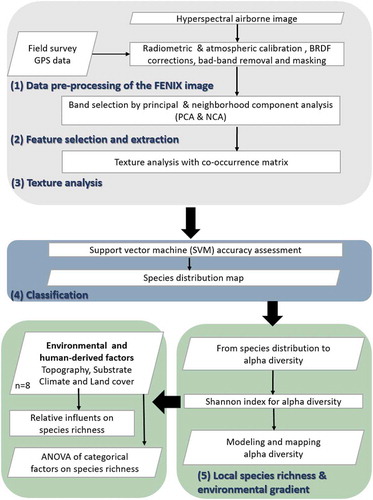
The methodology consists of five research stages (Figure 2): (1) pre-processing of the AISA-FENIX image, including atmospheric and radiometric calibrations, BRDF correction, masking procedure, and majority filter; (2) feature extraction and selection (FE&S): band selection by a combination of principal component and neighborhood component analyses; (3) texture parameterization with a co-occurrence matrix; (4) classification utilizing a support vector machine (SVM) of different band combinations and texture parameterizations and their accuracy assessments; and (5) mapping of the local species richness (i.e. alpha diversity) and analysis of their relationships with environmental and human-derived factors.

Figure 2. Study flowchart with the research stages implemented for species distribution and local species richness mapping along a climatic gradient

3.1 Feature extraction and selection

The FE&S method aims to improve prediction accuracy by selecting the essential spectral bands or features that contribute to species classification. FE&S are usually applied for several reasons: model simplification, reduction of training time, data dimensionality, and overfitting. Several studies have shown that hyperspectral data with a high spectral resolution are better than a small number of bands in identifying plant chemical compositions, potentially improving species identification (Torabzadeh, et al. 2014). However, high collinearity between the spectral bands and the noisy bands makes it essential to reduce their number by selecting only the diagnostic ones for spectral diversity (Wang and Gamon 2019). We used the principal component analysis (PCA) to evaluate bands number for reducing data dimensions and not as a method for feature (i.e. bands) selection . For band selection, we used the neighborhood component analysis (NCA) implemented on the original spectral bands (Yang et al.  2012). The PCA and NCA were applied in the Machine Learning Toolbox in Matlab 5.5 (Levy et al.  2019).

3.2 Texture analysis

Texture parameters reveal structural information related to crown properties, branching, and crown-internal shadows (Fassnacht et al. 2016). Previous studies showed that combining texture features with spectral information can improve species classification accuracy (Mallinis et al. 2008; Fassnacht et al. 2016). For example, Franklin et al. (2000) revealed that applying texture layers to species classification improved classification accuracy by 10–15%. We used eight well-known texture measures (Table 1), including mean, variance, homogeneity, contrast, dissimilarity, entropy, second moment, and correlation (Palubinskas and Reinartz 2011; Zhang et al. 2017; Culbert et al. 2012; Wood et al. 2012), as derived from the co-occurrence matrix utilized in ENVI 5.5 texture tools (ITT Visual Information Solutions, Boulder, CO, USA). The selection of the texture measures that best facilitate species classification was obtained using the previous section’s NCA technique.

Table 1. Texture expressions. $p\left(i,j\right)$ is the probability of a pixel’s (i, j) gray-level occurrence, $N_g$ is the number of distinct gray levels, and $\mu ,$ and $\sigma$indicate, the average and standard deviation within the kernel, respectively (Tahir et al. 2005)

Expression	Description	Expression	Description
Mean (1)	$\sum _{j=1}^{N_g}\sum _{j=1}^{N_g}i\times p\left(i,j\right)$	Variance (5)	$\sum _{j=1}^{N_g}\sum _{j=1}^{N_g}{\left(i-\mu \right)}^2\times p\left(i,j\right)$
Homogeneity (2)	$\sum _{j=1}^{N_g}\sum _{j=1}^{N_g}\frac{1}{1+{\left(i-j\right)}^2}\times p\left(i,j\right)$	Contrast (6)	$\sum _{j=1}^{N_g}\sum _{j=1}^{N_g}p\left(i,j\right)\times {\left(i-j\right)}^2$
Dissimilarity (3)	$\sum _{j=1}^{N_g}\sum _{j=1}^{N_g}p\left(i,j\right)\times \left|i-j\right|$	Entropy (7)	$\sum _{j=1}^{N_g}\sum _{j=1}^{N_g}p\left(i,j\right)\times \mathrm{l}\mathrm{o}\mathrm{g}\left(p\left(i,j\right)\right)$
Second Moment (4)	$\sum _{j=1}^{N_g}\sum _{j=1}^{N_g}{\left(p\left(i,j\right)\right)}^2$	Correlation (8)	$\frac{{\sum }_{j=1}^{N_g}{\sum }_{j=1}^{N_g}\left(ij\right)p\left(i,j\right)-{\mu }_x{\mu }_y}{{\sigma }_x{\sigma }_y}$

3.3 Support vector machine (SVM) classification

SVM is a well-known supervised machine-learning classification technique that offers significant advantages for species classification (Fassnacht et al. 2014; Paz-Kagan and Asner 2017). The ground truth data used for training the SVM model were grouped into nine dominant species (classes) and an additional category for other species related to tree and shrub species with a low abundance along the flight line. SVM classification was then implemented and tested for different spectral band combinations and texture measures. A linear SVM model was trained to find the optimal set of parameters to constrain computation time and avoid model overfitting using ENVI 5.5 software (Lamine et al. 2018). The kernel size and box remained constant to assess the model’s accuracy and enable us to compare the models with FE&S and texture analysis. The SVM classification accuracy was tested for the different spectral and textural feature combinations in an iterative process. The ground truth set was divided into training-testing datasets at a 50:50 split ratio selected randomly, followed by a post-classification accuracy assessment using the test group. The accuracy assessment included calculating the kappa coefficient and overall classification accuracy values for each species. The procedure was performed in the MATLAB machine learning toolbox 11.5 (Levy et al. 2019).

3.4 Effects of environmental and human-derived factors on local species richness

The local species richness mapping approach used here follows Féret and Asner (2014). The Shannon Index is a well-known index that combines species richness and evenness to estimate alpha (α) diversity (Wang et al. 2018). The SD map sample unit was divided into equally sized units by applying a kernel of 30 × 30 pixels to calculate the alpha diversity (Féret and Asner 2014). The Shannon Index Hʹ (Shanon and Weaver 1949) was calculated for each of these grid cells, using the following equation:

$H{ }^{\mathrm{\prime }}=-\sum _{i=1}^n{p}_i\times log\left(p_i\right)\left(9\right)$

where p_i represents the relative proportion of individual species, and i and n represent the total number of species for each 30 × 30 pixels (Paz‐Kagan et al. 2017).

3.5 Environmental and human-derived factors

To understand the determinants of local species diversity across the climatic gradient, we assessed the alpha diversity distributions with reference to available environmental and human-derived factors or information. The variables selected were:

• The topographical components were calculated from a digital elevation model (DEM) with a 4-m resolution from the Survey of Israel. Slope and aspect were calculated with the geo-morphometric and gradient metrics toolbox in ArcGIS (Rigol-Sanchez et al. 2015).

• The temperature map was based on land surface temperature (TIR radiance) from Landsat-8 image with a 100-m resolution acquired in proximity to the flight line time.

• The mean annual precipitation (MAP) map was based on 16 years of accumulated mean ‎yearly precipitation (mm per year). The Israel Meteorological Service developed the map, and the data collected from 131 stations around the country. ‎

• Substrata factors included soil type and lithology classification based on Official Survey of Israel data developed in 2004.

• The land-cover map was based on the Jewish National Fund (JNF) database.

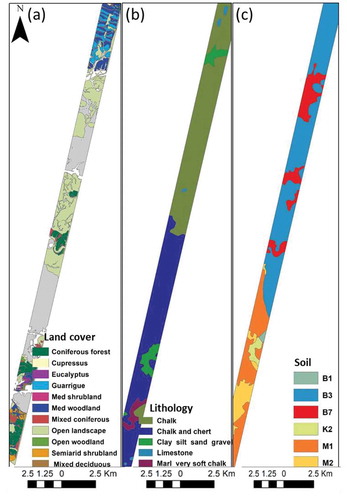
A detailed explanation of these input factors, their sources, and expected effects on species richness is given in Table 2, Figures 3 and Figures 4. The variables were all scaled up or down to have a similar spatial resolution of 30 m. The sensitivity of alpha diversity as an expression of the previously described habitat conditions was analyzed using Eureqa software (Dubčáková 2011). The sensitivity of the independent variable was calculated based on the partial derivative method (Mridula et al. 2018). In addition, the categorical factor was tested to evaluate alpha diversity differences. This analysis was based on 5000 pixels distributed randomly between the different categories, allowing a confidence level of 95%. The mean and standard error values were computed for each categorical variable, and their differences were compared. The statistical test was based on analysis of variance (ANOVA) and computed for the significant differences between the alpha diversity values for the categories’ factors based on Tukey’s honestly significant difference (HSD) test.

Table 2. Selected environmental and human-derived factors, their sources, and their expected effect on alpha diversity. ‎

Factor	Variable	Units	Source	The expected effect on alpha diversity
Environmental and human-derived	Land cover	Class	JNF forester maps	The spatial distribution and pattern of species diversity are affected by different land-cover types (Ohana-Levi et al. 2019)
	Land use	Class	Official Survey of Israel	Land-use activities transform natural areas into human-controlled landscapes, altering ‎species diversity and richness from the local to the global scale (Foley et al. 2005). The ‎land-use data in our study were used to mask agricultural and urban areas from the analysis.
Environmental	Elevation	m	Digital elevation model (DEM)	Elevation gradients are related to abiotic conditions, represent ‎complex interaction and variation. The typical distribution of species richness usually follows the elevation patterns (Beck et al. 2017).
	Aspect	Degree	Based on DEM	Slope steepness affects water distribution along a climatic gradient, where shallow slopes ‎are related to lower water discharge rates than steeper slopes, ‎altering species distribution and richness (Sternberg and Shoshany 2001).
	Slope	Degree	Based on DEM	The aspect was related to the radiation amount. The south-facing slopes receive higher ‎solar ‎radiation than the north-facing slopes in the northern hemisphere (Chhetri 2018). The ‎south-facing slopes are characterized by lower water availability and higher radiation, affecting ‎species distribution ‎between slopes-facing ‎ (Paz-Kagan et al. 2017).
	Temperature	C°	Land surface temperature (LST), derived from band 10 of Landsat-8	The temperature was found to be related to soil water content and is used for ‎‎estimating plant evapotranspiration. Water availability and temperature combination ‎are ‎often associated with species richness patterns along the elevation gradient ‎ (Beck et al. 2017).‎
	Mean annual precipitation	mm per year	16 years accumulated mean yearly precipitation from Israel Meteorological Service	The mean annual precipitation is related to water availability, plant water stress, ‎‎evapotranspiration rate, which affect species distribution and richness ‎ (O’Brien, et al.  2000).
	Soils	Class	Official Survey of Israel	Soil texture distribution influences the soil water holding capacity and soil moisture, which ‎results in soil water content distribution patterns affecting species distribution and ‎ richness (Ohana-Levi et al. 2019).
	Lithology	Class	Official Survey of Israel	Geology was related to soil chemistry, which influenced plant community ‎structure ‎ (Antonelli et al., 2018).

Figure 3. Environmental explanatory variables of local species richness: (a) aspect (degrees); (b) slope (degrees); (c) elevation (m); (d) land surface temperature (°C); (e) mean annual rainfall (mm/year)

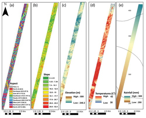
Figure 4. The categories of environmental and human-derived explanatory variables of local species richness: (a) land cover; (b) lithology; (c) soil type

4. Results

4.1 Feature extraction and selection

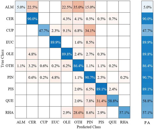
Table 3 presents the species distribution in the ground truth data as acquired during the field survey. As described earlier, a total of 247 woody crowns (i.e. trees and shrubs), with an average crown size of 20.2 m² and a total of 5134 pixels, were extracted from the hyperspectral image. The mean crown diameter for the nine dominant species (A. korschinskii, C. siliqua, E. camaldulensis, O. europaea, P. halepensis, P. lentiscus, and palaestina, Q. calliprinos, and R. lycioides) was approximately 5.7 m. The remaining low-abundance species (n = 14) were grouped into the “other” class. SVM mapping indicated that native shrubs (e.g. P. palaestina P. lentiscus, R. lycioides, and Q. calliprinos) were more frequently located in the northern part of the study area (Figure 5 (a)). The southern part is mainly occupied by planted species of P. halepensis and local C. sempervirens shrub species (Figure 5 (b)). The SVM classification for the test dataset showed a good performance without overfitting, with an overall accuracy of 86.1% using all 330 spectral bands. Figure 6 shows the confusion matrix for the nine dominant species along the flight line based on 330 spectral bands. The classification accuracy of six out of the nine dominant species showed high classification accuracy (C. silique (CER): 90%, E. camaldulensis (EUC): 89.9%, O. europaea (OLE): 89.9%, P. palaestina, and P. lentiscus (PIS): 89.1%, Q. calliprinos (QUE): 58.8%, and P. halepensis (PIN): 90.7%). The lowest accuracy was observed for A. korschinskii (ALM) (5%), represented by a relatively small number of crowns due to low abundance in the study area. The misclassification of C. sempervirens (CUP) (47.7%) was due to confusion with P. halepensis at a level of about 34%. The misclassification of R. lycioides (RHA) (57.1%) was due to confusion with other species (OTH) at about 28.6% (Fig .6).

Table 3. Training data for the support vector machine analysis of tree and shrub species mapped along the flight line. The classification was based on nine dominant species and one additional class of “other” that included less abundant species

Species name (abbreviation)	Number of crowns		Mean $\mathbf{a}\mathbf{n}\mathbf{d}\mathbf{S}\mathbf{D}$		Class
Amygdalus korschinskii (ALM)		11		28.7 $\pm$ 17.5	1
Ceratonia siliqua (CER)		29		28.8 $\pm$ 11.7	2
Eucalyptus camaldulensis (EUC)		20		18.6 $\pm$ 7.3	3
Cupressus sempervirens (CUP)		21		5.3 $\pm$ 0.8	4
Olea europaea (OLE)		22		$31.1\pm$ 17.3	5
Pinus halepensis (PIN)		44		17.8 $\pm$ 8.9	6
Pistacia lentiscus and palaestina (PIS)		22		28.2 $\pm$ 15.1	7
Quercus calliprinos (QUE)		19		21.7 $\pm$ 11.5	8
Rhamnus lycioides (RHA)		18		12.0 $\pm$ 4.5	9
Acacia saligna (ACA)		2		15.6 $\pm$ 6.3	Other
Atriplex halimus (ATR)		3		9.8 $\pm$ 2.5
Cercis siliquastrum (CEC)		2		17.7 $\pm$ 5.1
Melia azedarach (MEL)		3		14.9 $\pm$ 3.5
Mixed Dense dwarf shrub (DDS)		5		47.5 $\pm$ 12.4
Mixed Sparse dwarf shrub (SDS)		5		15.5 $\pm$ 6.2
Nerium oleander (NER)		3		14.7 $\pm$ 3.1
Phillyrea latifolia (PHY)		6		15.1 $\pm$ 5.6
Retama raetam (RET)		3		8.7 $\pm$ 3.1
Spartium junceum (SPA)		2		10.0 $\pm$ 1.0
Sarcopoterium spinosum (SAC)		5		4.5 $\pm$ 1.3
Ziziphus spina-christi (ZIZ)		2		26.5 $\pm$ 2.1
Total		247		20.2$\pm$ 13.4

Figure 5. Species distribution (SD) maps of the nine dominant species along the flight line. Native woodland was more abundant in the northern region (a), while planted trees were highly abundant in the southern region (b)

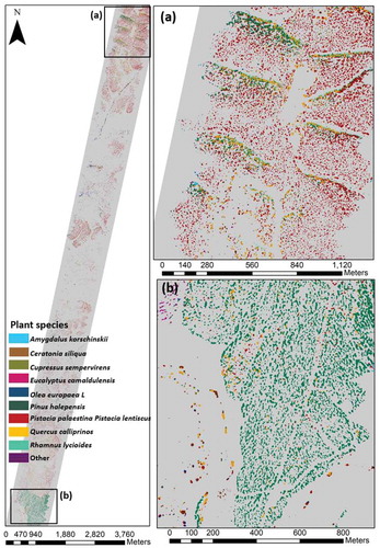
Figure 6. Confusion matrix for the nine dominant species along the flight line for the SVM model based on 330 spectral bands. The species classes are Amygdalus korschinskii (ALM), Ceratonia siliqua (CER), Eucalyptus camaldulensis (EUC), Cupressus sempervirens (CUP), Olea europaea (OLE), Pinus halepensis (PIN), Pistacia lentiscus and Pistacia palaestina (PIS), Quercus calliprinos (QUE), and Rhamnus lycioides (RHA). PA refers to prediction accuracy

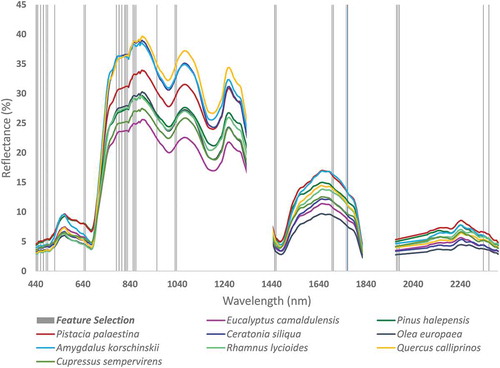
The PCA served to determine diagnostic wavelength bands for species identification, which yield combinations of 330, 33, 22, 15, and 11 spectral bands. We tested the classification accuracy assessment based on SVM models corresponding to the number of bands selected by the PCA models shown in Table 4. Although only 33 principal components (PC) were selected from the linear combinations of the original bands that were used instead of 330 spectral bands, the difference in accuracy was less than 2% (84.2%) and less than 7% (79.2%) for 15 spectral bands. This means that using only 10% of the spectral data (i.e. 33 original spectral bands) could yield a relatively accurate classification model based on linear transformation. Thus, we applied NCA to the original bands for selecting 33 bands and 15 bands, which included the following spectral bands (μm): 0.439, 0.443, 0.449, 0.456, 0.463, 0.466, 0.483, 0.555, 0.558, 0.634, 0.641, 0.647, 0.654, 0.658, 0.661, 0.675, 0.678, 0.682, 0.734, 0.778, 0.782, 1.070, 1.076, 1.330, 1.336, 1.342, 1.500, 1.506, 1.726, 1.732, 1.738, 2.375, and 2.399. The 15 features that were selected are highlighted in bold. Figure 7 shows the average spectral signatures of nine dominant species and the features that were selected. Despite the differences in their reflectance levels, the spectral signatures are relatively similar, demonstrating the main difficulty in species identification and highlighting the need to select specific absorption features (i.e. spectral bands). Table 5 shows SVM classification accuracy results for 330 and 33 selected spectral bands based on FE&S with their prediction accuracy and user accuracy for the nine dominant species. Appendix 1 shows the confusion matrix for the nine dominant species along the flight line based on 33 spectral bands.

Table 4. The accuracy assessment corresponding to the number of spectral bands selected by principal components analysis was based on the principal components (PCs)

Number of spectral bands	330	33	22	15	11
Overall Accuracy (%)	86.1	84.2	81.4	79.2	68.6

Table 5. The SVM classification accuracy for 330 spectral bands and 33 selected spectral bands was based on principal components analysis. PA refers to prediction accuracy, and UA refers to user accuracy

Species class	330 bands		33 bands
	PA (%)	UA (%)	PA (%)	UA (%)
ALM	5.0	25.0	5.1	33.3
CER	90.0	90.2	90.9	86.6
CUP	47.7	84.0	67.4	100.0
EUC	89.9	91.3	82.3	82.0
OLE	89.8	79.9	82.9	79.7
OTH	86.4	86.8	84.7	83.2
PIN	90.7	84.1	85.0	80.5
PIS	89.1	87.0	80.2	92.5
QUE	58.8	73.2	86.3	71.0
RHA	57.1	95.2	77.1	75.0
OA (%)	86.1		84.2

Figure 7. Mean spectral signatures of the nine dominant species woody species with band feature extraction and selection indicated in vertical gray lines

4.2 Texture analysis

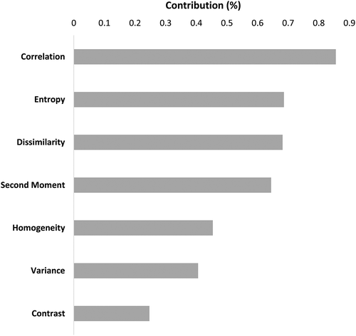
Texture analysis was applied to the seven dominant species, considering the 54 relatively large crowns of over 5 m in diameter (C. sempervirens and R. lycioides were excluded due to their small crown sizes). The crowns included, overall, 913 pixels and a total of 231 texture bands that were used for the analysis (33 bands multiplied by the seven texture measures: variance, homogeneity, contrast, dissimilarity, entropy, second moment, and correlation, excluding mean) (Zhang et al. 2008). The NCA was applied to the 231 bands to choose the essential texture measures, yielding the four texture measures: correlation, entropy, dissimilarity, and second moment. Appendix 2 shows the relative contribution of texture parameters to the classification accuracy. It was noted that the correlation measure was higher in classification accuracy than any of the other texture measures. The results showed that using only correlation parameter and 33 selected spectral bands, the overall accuracy reached 92.8% (Table 6). The results present the SVM classification accuracy assessment using different combinations of reflectance and texture measures. When reflectance was combined with only the correlation measure, the accuracy was high and almost as high as when reflectance was combined with all other texture parameterizations (Table 6). Consequently, combining the correlation measure with reflectance is sufficient to improve species classification. However, several of the texture expressions (e.g. contrast) impede species identification, negatively impacting the model performance (called “overfitting”). Table 6 shows the overall classification accuracy assessments using a combination of reflectance data following FE&S and texture analysis as applied on SVM results. The texture information for both kernel sizes 3 and 5 showed very similar accuracy, as seen in Table 6. Combining texture information with the reflectance data of 33 bands with texture bands calculated with a kernel size of 3 × 3 pixels improves the classification accuracy by more than 7.1% to 93.3 for the seven dominant species only (crown diameter higher than 5 m).

Table 6. Classification accuracy assessment using a combination of reflectance data, based on feature extraction and selection of the 33 spectral bands and texture analysis using SVMs. Note that these results refer only to large-canopy species (> 5 m)

	Reflectance for 33 spectral bands	All texture (3 × 3)	Combined reflectance & all texture (3 × 3)	Combined reflectance & only correlation (3 × 3)	Combined reflectance & only correlation (5 × 5)
Overall accuracy	86.2%	65.8%	93.3%	92.8%	90.2%

4.3 Environmental and human-derived factors

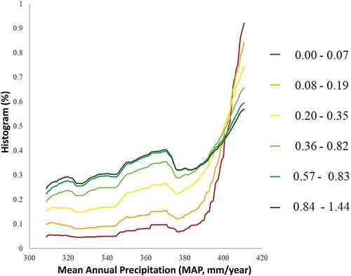
Figure 8 presents the results of the alpha diversity (based on equation 9) maps along the climatic gradient ranging between 0.01 and 1.44. In general, high index values were found in the high-density region on the north-facing slope and in the northern part of the flight line (Figure 8 (a)). The environmental factor with the highest sensitivity to the alpha diversity index was MAP, notably higher than slope, surface temperature, aspect, and elevation (Figure 9). Figure 10 shows the normalized histogram for each alpha range classified into six classes, characterizing the rainfall gradient. As the MAP increases, all alpha class frequencies increase, indicating that the richness is significantly associated with annual rainfall. Interestingly, most alpha classes showed a similar percentage near 400 mm.

Figure 8. Local species richness (alpha diversity) map based on the Shannon Index throughout the study sites: (a) native woodland in the northern region; and (b) planted trees in the southern region

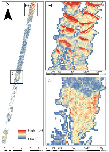
Figure 9. The five selected environmental factors’ sensitivities corresponding to the alpha diversity index along the climatic gradient. MAP stands for mean annual precipitation

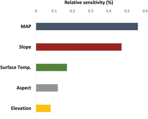
Figure 10. Normalized histogram for each range of alpha diversity versus mean annual precipitation (MAP) (mm/year) in the study area

Figure 11 shows soil (a) and lithology (b) differences in the alpha diversity response. Alpha diversity was significantly higher in the northern part of the climatic gradient. The dominant soil type in this region is light and brown Rendzina, and the lithology is characterized by chalk that covers most of the northern part. The vegetation cover type showed significantly higher species richness in the natural Mediterranean shrublands and the guarrigue plant community, where the lowest species richness was found in the open woodlands and the open landscapes (Figure 12). Utilizing the existing ecological map by the proportional cover of the Mediterranean shrubland was found relatively low in the study area, with an overall 2% cover. In contrast, the guarrigue (i.e. natural Mediterranean shrubland and woodland) covered more than 15% of the study area (Table 7).

Table 7. List of categorical factors of vegetation cover, soil, and lithology, their class description, and percentage cover in the study area

Parameter	Class	Percent cover (%)	Description
Vegetation cover	Cypresses	0.83	Planted cypresses
	Semi-arid shrubland	4.5	Semi-arid dwarf-shrubland (batha)
	Eucalyptus	1.65	Planted eucalyptus
	‎Mixed deciduous	1.62	Natural mixed coniferous and deciduous forest
	Guarrigue	15.75	Natural Mediterranean shrubland and woodland
	Med shrubland	2.05	Natural Mediterranean dwarf-shrubland (batha)
	Med woodland	27.39	Natural Mediterranean woodland
	Mixed coniferous	9.83	Mixed coniferous
	Open landscape	3.63	Open area with sparse woody vegetation
	Open woodland	2.64	Open woodland
	Coniferous forest	30.2	Planted coniferous (pine) forest
Lithology	Chalk	43.42	Chalk
	Chalk and chart	53.45	Chalk and chart
	Clay silt sand	2.02	Clay silt sand gravel (Alluvium soil)
	Limestone	0.29	Limestone
	Marl	0.817	Marl very soft chalk
Soil	B1	0.29	Brown Randzina
	B3	42	Light Randzina
	B7	0.54	Derek Gromosols
	K2	2.86	Gromosol dark brown soils
	M1	30.22	Loess soil
	M2	24.08	Light loess soils

Figure 11. The selected factors of lithology and soil type corresponding to alpha diversity. Significant differences are marked with asterisks (p ≤ 0.05). ns stands for no significant

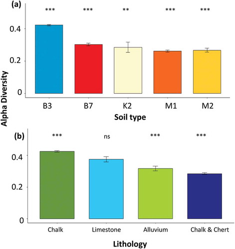
Figure 12. The selected factor of the land cover type corresponding to alpha diversity. Significant differences are marked with asterisks (p ≤ 0.05). ns stands for no significant

5. Discussion

The study aims were, first, to improve trees and shrub species classification using airborne hyperspectral imagery in heterogeneous Mediterranean environments, secondly, to map their richness, and thirdly, to assess habitat alpha diversity variation determinants. A detailed field survey was acquired for high spatial resolution hyperspectral strips for a Mediterranean region. One of the challenges of SD modeling in Mediterranean areas concerns spatial heterogeneity and the relatively small tree and shrub size. We showed that integrating textural analysis and FE&S improved the SD classification accuracy by more than 7% for the seven dominant species with a crown diameter larger than 5 m. We used the approach suggested by Féret and Asner (2014) of spectral diversity and tested its variation in response to habitat (i.e. climatic, topography, and substrate) and human-derived factors (i.e. land-cover factors). Mean annual precipitation was the most sensitive factor to alpha diversity, where alpha class frequency increased with the increase in MAP, representing species diversity associated with the annual rainfall gradient. Low alpha-diversity values were primarily related to MAP. The alpha diversity showed substantially higher species richness in the natural Mediterranean shrubland and the guarrigue, mainly located in the northern part of the climate gradient.

5.1 Feature selection and extraction

Finding the essential spectral bands (FE&S) for plant species detection plays a critical role in improving species classification accuracy and developing an analytical approach for SD mapping. Previous studies that applied FE&S to hyperspectral data showed general improvement in the classification accuracy (Alonzo et al.  2014; Fassnacht et al. 2016). SVM classification relies on specific bands related to the biochemical concentration and spectral features of leaf chemistry. These include spectral information on available water content (970, 1100, 1200 nm), chlorophyll pigments (500 nm), nitrogen (1500, 1700 nm), and carbon, cellulose, and lignin (2020, 2150, and 2350 nm, respectively) (Baldeck and Asner 2013; Asner and Martin 2015; Paz-Kagan and Asner 2017; Paz-Kagan et al. 2017). Fassnacht et al. (2016) summarize 13 studies that make use of IS and FE&S for species mapping, showing that the essential spectral bands mainly overlap with features related to water content and plant photosynthetic pigments. Our results concerning the essential wavelengths are in good agreement with these studies. Using the optimal number of spectral bands reduces the SD classification accuracy by about 2% (84.2), with only 10% of the spectral data (33 spectral bands). These results can help select the essential features (spectral bands) and contribute to model simplification by reducing training time, data dimensionality, and data overfitting. Moreover, FE&S is necessary to develop future satellite missions and select the relevant spectral bands to improve species classification ability (Rocchini et al. 2021, 2016). Such tasks may contribute to mapping woody species over vast regions by integrating airborne-based IS and satellite data.

5.2 Texture analysis

An additional aspect of species classification is the structural aspect of the tree or shrub. Texture analysis is also an essential topic in species classification both for ecology and remote sensing, especially in the Mediterranean and desert-fringe ecosystems (Shoshany 2000). The crown-structure parameters, such as size, density, and shadow effects, are all texture information that affects species classification (Fassnacht et al. 2016). In the last decade, high spatial resolution IS data (airborne-based) have been used mainly for SD mapping. However, these data depend on regional environmental characterization, vegetation coverage, and structure (Wang and Gamon 2019). Combining spectral band selection features and texture analysis improves the accuracy of species ‎identification ‎ (Mallinis et al. 2008). Several studies have shown that texture analysis can improve species classification accuracy by up to 10%–15% (Fassnacht et al. 2016). However, since texture analysis has multiscale perspectives and expressions, the kernel window size must be optimized for the study area. It is affected by site-specific species characteristics related to crown size, structure, and density (Fassnacht et al. 2016). Therefore, there was a trade-off between spatial resolution and species classification, mainly in areas where the tree and shrub sizes are relatively small. We showed that using only 33 spectral bands, with all the texture parameters, improved the classification accuracy by 7.1% and reached 93.3% classification accuracy for the seven dominant species with a crown diameter larger than 5 m. In addition, the classification accuracy was 92.8% using only correlation measures of texture parameters, and the 33 selected spectral bands showed almost as high accuracy as with all the texture parameters together (93.3%). Studies have shown that different texture features and window sizes could affect species classification accuracy (Fassnacht et al. 2016; Ferreira et al. 2019). Therefore, selecting appropriate texture analysis, careful selection of input bands, and establishing a suitable classification algorithm are essential tasks for species classification mapping (Ferreira et al. 2019). Consequently, we suggest that future studies should test the effect of vegetation structure on kernel window size and texture features analysis to reveal species classification accuracy cusses. In the current study, we used only two kernel sizes that are insufficient to draw a conclusion. However, the effect of different kernel sizes for texture combinations for species classification is proposed to be studied in the future. We recommend that future research efforts focus on integrating information from various sensors for species classification while understanding the causes of their advantages or disadvantages under certain conditions. Integrating additional information based on light detection and ranging (LiDAR) could significantly contribute to species classification (Marrs and Ni-Meister 2019; Asner and Martin 2008). LiDAR is increasingly utilized to collect data on the structural features of woody vegetation. The current technological development of higher resolution UAV images and hyperspectral images and LiDAR could make SD modeling more accessible in the coming years in areas with relatively small woody vegetation, such as in our case study (Wallace et al. 2016).

5.3 From species distribution to local species richness

Remote-sensing spectral diversity is based on a similar approach of alpha diversity that replaces ‎the species attributes with spectral data (Feilhauer and Schmidtlein 2009; Dogan and Dogan 2006). Several models were developed to map alpha diversity using spectral reflectance data, and we used the approach suggested by Féret and Asner (2011). Plant diversity is shaped in space and time more by climate aspects than by any other factor (Laliberté et al. 2020). In our study area, we found that the MAP had the highest sensitivity to alpha diversity. Water is a critical limiting resource in the Mediterranean to semi-arid regions, and its availability shapes plant diversity and primary productivity (Harrison et al. 2020). In these regions, the climate is rapidly changing toward higher temperatures and less water availability during the growing season (McLaughlin et al. 2017), thus making these areas drier under this combination (Harrison et al. 2020). Climate change is expected to alter plant diversity patterns by affecting phenology, species composition, and community structure, which has been well documented in the past due to direct and indirect effects across multiple scales (Titeux et al. 2017; Ihlow et al. 2012; Harrison et al. 2020). Therefore, given the rapidity of current environmental change, applying remote sensing techniques to monitor spectral diversity along climatic gradients is more crucial than ever. The second environmental factor affecting the alpha diversity index was the slope, which affects water distribution. Steep slopes increase the water discharge rates than shallow slopes, affecting ‎the local species pool. Slope and aspect were found to be connected to soil moisture and solar radiation. Studies ‎have shown that north-facing slopes substantially affect the composition, structure, and density of ‎plant community development in Mediterranean regions ‎ (Govigli et al. 2020). These factors were associated with the decrease in plant biomass along the Mediterranean gradient, corresponding with reductions in rainfall and increases in the water deficit (Kadmon and Danin 1999). The third environmental factor affecting alpha diversity was the land surface temperature, which indicated that the surface temperature increases when plant species diversity and cover decreases.

Climate change and species diversity are complex, and many aspects remain unclear (Bellard et al. 2012). However, the effect of human-derived factors increases this complexity. We found that the Mediterranean shrubland and the guarrigue areas, located mainly in the northern part of the elevation gradient, had the highest richness, while the planted forest had lower diversity. Human-derived factors raise additional aspects that need to be considered, such as identifying edge-effects, habitat fragmentation, and the interaction of invasive species, which all require further study (Paz‐Kagan et al. 2017; Paz-Kagan et al. 2019; Shoshany, 2002; Kutiel et al., 2000). The impact of land use and habitat fragmentation is widespread in the study area. Future study is needed to understand their effect on local and regional species richness (alpha and beta diversity). As land use and fragmentation intensify and become more widespread in these regions, their impact on ecosystem function, structure, and services will increase at the local and regional scales (Lambin et al. 2001). The combination of SD and richness and knowledge of land use and cover will improve the ability to understand their interaction with climate effects. Therefore, spectral diversity applications could become a valuable remote sensing tool for biodiversity alteration and‎ conservation strategies under climate and land-use changes.

6. Conclusions

For the last decade, extensive research has been dedicated to using remote sensing techniques for spectral species diversity estimation (Fassnacht et al. 2016). Spectral diversity modeling based on IS provides valuable information for conservation in highly heterogeneous areas such as the Mediterranean ecosystem. This information is especially relevant for natural woodland and shrublands in the Mediterranean regions with high species diversity and relatively small areas that remain undisturbed. In this paper, we investigated several knowledge gaps related to IS-based SD and richness mapping. SD mapping was recognized, and ways to improve its classification accuracy were suggested. These could help achieve more accurate SD mapping to support management strategies by identifying the hotspot regions of species diversity. The geographical pattern in alpha diversity was studied, and its relation to different environmental and human-derived factors was presented. We found that the alpha diversity increases with increased rainfall, despite the decrease in temperatures, consistent with other studies on climate-richness patterns. The geographical patterns identified here have all been documented previously, but such a long-dimension climate gradient is a unique case study that can aid in understanding the expected changes through “Space” thinking in similar regions.

Highlights

• Species diversity was tested using hyperspectral data along a climatic ‎gradient

• Bands selection for species distribution classification were tested using feature ‎selection

• Texture analysis was performed to obtain the structural information

• Alpha diversity was tested in response to environmental and human-driven factors

• The factor with the highest sensitivity to alpha diversity was mean annual ‎precipitation

Acknowledgements

The authors thank Mr. Ofer Cohen for his assistance with species identification and Mr. Alexander Goldberg for GPS measurements and field data collection. The support of the Helen and Norman Asher Space Research Fund (no.907014) is highly appreciated and the support of the VENuS research of the Israel Space Agency, Ministry of Science and Technology Israel (no. 3-14722).

Disclosure statement

The authors have declared that they have no competing interests.

Appendices 1.

Confusion matrix for the nine dominant species along the flight line for the support vector machine (SVM) model based on 33 spectral bands. The species classes: Amygdalus korschinskii (ALM), Ceratonia siliqua (CER), Eucalyptus camaldulensis (EUC), Cupressus sempervirens (CUP), Olea europaea (OLE), Pinus halepensis (PIN), Pistacia lentiscus and Pistacia palaestina (PIS), Quercus calliprinos (QUE), and Rhamnus lycioides (RHA). PA refers to prediction accuracy

Appendices 2.

The results of the relative contribution of texture parameters to the classification accuracy

References

- Alonzo, M., B. Bookhagen, and D. A. Roberts. 2014. “Urban Tree Species Mapping Using Hyperspectral and Lidar Data Fusion.” Remote Sensing of Environment. 148: 70–83.
- Antonelli, A., A. Zizka, F. A. Carvalho, R. Scharn, C. D. Bacon, D. Silvestro, and F. L. Condamine. 2018. “Amazonia is the primary source of Neotropical biodiversity.” Proceedings of the National Academy of Sciences 115 (23): 6034–6039.
- Asner, G., and R. Martin. 2015. “Spectroscopic Remote Sensing of Non-Structural Carbohydrates in Forest Canopies.” Remote Sensing 7 (4): 3526. doi:https://doi.org/10.3390/rs70403526.
- Asner, G. P., and R. E. Martin. 2008. “Airborne Spectranomics: Mapping Canopy Chemical and Taxonomic Diversity in Tropical Forests.” Frontiers in Ecology and the Environment 7 (October): 269–276. doi:https://doi.org/10.1890/070152.
- Asner, G. P., R. E. Martin, D. E. Knapp, R. Tupayachi, C. B. Anderson, F. Sinca, N. R. Vaughn, and W. Llactayo. 2017. “Airborne Laser-Guided Imaging Spectroscopy to Map Forest Trait Diversity and Guide Conservation.” Science 355 (6323): 385–389. doi:https://doi.org/10.1126/science.aaj1987.
- Baldeck, C., and G. Asner. 2013. “Estimating Vegetation Beta Diversity from Airborne Imaging Spectroscopy and Unsupervised Clustering.” Remote Sensing 5 (5): 2057. doi:https://doi.org/10.3390/rs5052057.
- Barredo, J. I., G. Caudullo, and A. Dosio. 2016. “Mediterranean Habitat Loss under Future Climate Conditions: Assessing Impacts on the Natura 2000 Protected Area Network.” Applied Geography 75. Elsevier: 83–92. doi:https://doi.org/10.1016/j.apgeog.2016.08.003.
- Baudena, M., A. Sánchez, C.-P. Georg, P. Ruiz-Benito, M. Á. Rodríguez, M. A. Zavala, and M. Rietkerk. 2015. “Revealing Patterns of Local Species Richness along Environmental Gradients with a Novel Network Tool.” Scientific Reports 5 (1). Nature Publishing Group: 1–15. doi:https://doi.org/10.1038/srep11561.
- Beck, J., M. Christy, M. J. C. Axmacher, L. A. Ashton, F. Bärtschi, G. Brehm, S. Choi, O. Cizek, R. K. Colwell, and F. Konrad. 2017. “Elevational Species Richness Gradients in A Hyperdiverse Insect Taxon: A Global Meta‐study on Geometrid Moths.” Global Ecology and Biogeography 26 (4). Wiley Online Library: 412–424. doi:https://doi.org/10.1111/geb.12548.
- Bellard, C., C. Bertelsmeier, P. Leadley, W. Thuiller, and F. Courchamp. 2012. “Impacts of Climate Change on the Future of Biodiversity.” Ecology Letters 15 (4). Wiley Online Library: 365–377.
- Chang, J., and M. Shoshany. 2017. “Radar Polarization and Ecological Pattern Properties across Mediterranean-to-Arid Transition Zone.” Remote Sensing of Environment 200. doi:https://doi.org/10.1016/j.rse.2017.08.032.
- Chang, J. G., M. Shoshany, and O. Yisok. 2018. “Polarimetric Radar Vegetation Index for Biomass Estimation in Desert Fringe Ecosystems.” IEEE Transactions on Geoscience and Remote Sensing PP. IEEE: 1–7. doi:https://doi.org/10.1109/TGRS.2018.2848285.
- Chhetri, P. K. 2018. “Predicting upslope expansion of sub-alpine forest in the Makalu Barun National Park, Eastern Nepal, with a hybrid cartographic model”. Journal of forestry research 29 (1): 129–137.
- Chiarucci, A., S. Fattorini,B. Foggi,S. Landi,L. Lazzaro,J. Podani,D. Simberloff. 2017. “Plant recording across two centuries reveals dramatic changes in species diversity of a Mediterranean archipelago‟. Scientific reports, 7(1): 1–11.
- Culbert, P. D., V. C. Radeloff, V. St-Louis, C. H. Flather, C. D. Rittenhouse, T. P. Albright, and A. M. Pidgeon. 2012. “Modeling Broad-Scale Patterns of Avian Species Richness across the Midwestern United States with Measures of Satellite Image Texture.” Remote Sensing of Environment 118. Elsevier: 140–150. doi:https://doi.org/10.1016/j.rse.2011.11.004.
- Da, S. S., J. R. G. Márquez, J. H. Sommer, A. Thiombiano, G. Zizka, S. Dressler, M. Schmidt, C. Chatelain, and W. Barthlott. 2018. “Plant Biodiversity Patterns along a Climatic Gradient and across Protected Areas in West Africa.” African Journal of Ecology 56 (3). Wiley Online Library: 641–652. doi:https://doi.org/10.1111/aje.12517.
- Danin, A., G. Orshan, and M. Zohary. 1975. “Vegetation of the Northern Negev and the Judean Desert of Israel.” Israel Journal of Botany.
- De Bello, F., J. Lepš, and S. Maria‐Teresa. 2006. “Variations in Species and Functional Plant Diversity along Climatic and Grazing Gradients.” Ecography 29 (6). Wiley Online Library: 801–810. doi:https://doi.org/10.1111/j.2006.0906-7590.04683.x.
- Dogan, H. M., and M. Dogan. 2006. “A New Approach to Diversity Indices–Modeling and Mapping Plant Biodiversity of Nallihan (A3-ankara/turkey) Forest Ecosystem in Frame of Geographic Information Systems.” Biodiversity and Conservation 15 (3). Springer: 855–878. doi:https://doi.org/10.1007/s10531-004-2937-4.
- Dubčáková, R. 2011. “Eureqa: Software Review.” Springer.
- Evenari, M., I. Noy-Meir, and D. W. Goodall. 1985. “Hot Deserts and Arid Shrublands.” Ecosystems of the World :12. Amsterdam, Netherlands: Elsevier.
- Fassnacht, F. E., C. Neumann, M. Förster, H. Buddenbaum, A. Ghosh, A. Clasen, P. K. Joshi, and B. Koch. 2014. “Comparison of Feature Reduction Algorithms for Classifying Tree Species with Hyperspectral Data on Three Central European Test Sites.” IEEE Journal of Selected Topics in Applied Earth Observations and Remote Sensing 7 (6). IEEE: 2547–2561. doi:https://doi.org/10.1109/JSTARS.2014.2329390.
- Fassnacht, F. E., H. Latifi, K. Stereńczak, A. Modzelewska, M. Lefsky, L. T. Waser, C. Straub, and A. Ghosh. 2016. “Review of Studies on Tree Species Classification from Remotely Sensed Data.” Remote Sensing of Environment 186: 64–87. doi:https://doi.org/10.1016/j.rse.2016.08.013.
- Feilhauer, H., and S. Schmidtlein. 2009. “Mapping Continuous Fields of Forest Alpha and Beta Diversity.” Applied Vegetation Science 12 (4). Wiley Online Library: 429–439. doi:https://doi.org/10.1111/j.1654-109X.2009.01037.x.
- Féret, J.-B., and G. P. Asner. 2011. “Spectroscopic Classification of Tropical Forest Species Using Radiative Transfer Modeling.” Remote Sensing of Environment 115 (9). Elsevier: 2415–2422. doi:https://doi.org/10.1016/j.rse.2011.05.004.
- Féret, J.-B., and G. P. Asner. 2014. “Mapping Tropical Forest Canopy Diversity Using High‐fidelity Imaging Spectroscopy.” Ecological Applications 24 (6). Wiley Online Library: 1289–1296. doi:https://doi.org/10.1890/13-1824.1.
- Ferreira, M. P., F. H. Wagner, L. E. O. C. Aragão, Y. E. Shimabukuro, and F. Carlos Roberto de Souza. 2019. “Tree Species Classification in Tropical Forests Using Visible to Shortwave Infrared WorldView-3 Images and Texture Analysis.” ISPRS Journal of Photogrammetry and Remote Sensing 149. Elsevier: 119–131. doi:https://doi.org/10.1016/j.isprsjprs.2019.01.019.
- Foley, J. A., R. DeFries, G. P. Asner, C. Barford, G. Bonan, S. R. Carpenter, F.S. Chapin, M. T. Coe, G. C. Daily, and H. K. Gibbs. 2005. “Global consequences of land use”. Science (80) 309: 570–574.
- Franklin, S. E., R. J. Hall, L. M. Moskal, A. J. Maudie, and M. B. Lavigne. 2000. “Incorporating Texture into Classification of Forest Species Composition from Airborne Multispectral Images.” International Journal of Remote Sensing 21 (1). Taylor & Francis: 61–79. doi:https://doi.org/10.1080/014311600210993.
- Gillespie, T. W., G. M. Foody, D. Rocchini, A. P. Giorgi, and S. Saatchi. 2008. “Measuring and Modelling Biodiversity from Space.” Progress in Physical Geography 32 (2): 203–221. doi:https://doi.org/10.1177/0309133308093606.
- Goetz, A. F. H., G. Vane, J. E. Solomon, and B. N. Rock. 1985. “Imaging Spectroscopy for Earth Remote Sensing.” Science 228 (4704): 1147–1153. doi:https://doi.org/10.1126/science.228.4704.1147.
- Govigli, M., V. J. R. Healey, J. L. G. Wong, K. Stara, R. Tsiakiris, and J. M. Halley. 2020. “When Nature Meets the Divine: Effect of Prohibition Regimes on the Structure and Tree Species Composition of Sacred Forests in Northern Greece.” Web Ecology 20 (2). Copernicus GmbH: 53–86. doi:https://doi.org/10.5194/we-20-53-2020.
- Harrison, J. L., A. B. Reinmann, A. S. Maloney, N. Phillips, S. M. Juice, A. J. Webster, and P. H. Templer. 2020. “Transpiration of Dominant Tree Species Varies in Response to Projected Changes in Climate: Implications for Composition and Water Balance of Temperate Forest Ecosystems.” Ecosystems: 1–16.
- Harrison, S., M. J. Spasojevic, and L. Daijiang 2020. “Climate and Plant Community Diversity in Space and Time.” Proceedings of the National Academy of Sciences 117 ( 9). National Acad Sciences: 4464–4470.
- He, K. S., B. A. Bradley, A. F. Cord, D. Rocchini, M. Tuanmu, S. Schmidtlein, W. Turner, M. Wegmann, and P. Nathalie. 2015. “Will Remote Sensing Shape the Next Generation of Species Distribution Models?” Remote Sensing in Ecology and Conservation 1 (1). Wiley Online Library: 4–18. doi:https://doi.org/10.1002/rse2.7.
- Ihlow, F., J. Dambach, J. O. Engler, M. Flecks, T. Hartmann, S. Nekum, H. Rajaei, and R. Dennis. 2012. “On the Brink of Extinction? How Climate Change May Affect Global Chelonian Species Richness and Distribution.” Global Change Biology 18 (5). Wiley Online Library: 1520–1530. doi:https://doi.org/10.1111/j.1365-2486.2011.02623.x.
- Kadmon, R., and A. Danin. 1999. “Distribution of Plant Species in Israel in Relation to Spatial Variation in Rainfall.” Journal of Vegetation Science 10 (3). Wiley Online Library: 421–432. doi:https://doi.org/10.2307/3237071.
- Kutiel, P., H. Kutiel, and H. Lavee. 2000. “Vegetation Response to Possible Scenarios of Rainfall Variations along a Mediterranean–Extreme Arid Climatic Transect.” Journal of Arid Environments 44 (3). Elsevier: 277–290. doi:https://doi.org/10.1006/jare.1999.0602.
- Laliberté, E., A. K. Schweiger, P. Legendre, and F. He. 2020. “Partitioning Plant Spectral Diversity into Alpha and Beta Components.” Ecology Letters 23 (2). Wiley Online Library: 370–380. doi:https://doi.org/10.1111/ele.13429.
- Lambin, E. F., B. L. Turner, H. J. Geist, S. B. Agbola, A. Angelsen, J. W. Bruce, O. T. Coomes, R. Dirzo, G. Fischer, and C. Folke. 2001. “The Causes of Land-Use and Land-Cover Change: Moving beyond the Myths.” Global Environmental Change 11 (4). Elsevier: 261–269. doi:https://doi.org/10.1016/S0959-3780(01)00007-3.
- Lamine, S., G. P. Petropoulos, S. K. Singh, S. Szabó, N. E. I. Bachari, P. K. Srivastava, and S. Suman. 2018. “Quantifying Land Use/Land Cover Spatio-Temporal Landscape Pattern Dynamics from Hyperion Using SVMs Classifier and FRAGSTATS®.” Geocarto International 33 (8). Taylor & Francis: 862–878. doi:https://doi.org/10.1080/10106049.2017.1307460.
- Levy, M., D. Raviv, and J. Baker. 2019. “Data Center Predictions Using Matlab Machine Learning Toolbox.” In 2019 IEEE 9th Annual Computing and Communication Workshop and Conference (CCWC), 458–464. IEEE. Las-Vegas, NA, USA.
- Li, L., Y. Zhang, W. Jianshuang, L. Shicheng, B. Zhang, Z. Jiaxing, H. Zhang, M. Ding, and B. Paudel. 2019. “Increasing Sensitivity of Alpine Grasslands to Climate Variability along an Elevational Gradient on the Qinghai-Tibet Plateau.” Science of the Total Environment 678. Elsevier: 21–29. doi:https://doi.org/10.1016/j.scitotenv.2019.04.399.
- Lu, D., Q. Weng, E. Laliberté, A. K. Schweiger, and P. Legendre. 2007. “A Survey of Image Classification Methods and Techniques for Improving Classification Performance.” International Journal of Remote Sensing 28 (October): 823–870. doi:https://doi.org/10.1080/01431160600746456.
- Mallinis, G., N. Koutsias, M. Tsakiri-Strati, and M. Karteris. 2008. “Object-Based Classification Using Quickbird Imagery for Delineating Forest Vegetation Polygons in a Mediterranean Test Site.” ISPRS Journal of Photogrammetry and Remote Sensing 63 (2). Elsevier: 237–250. doi:https://doi.org/10.1016/j.isprsjprs.2007.08.007.
- Marrs, J., and W. Ni-Meister. 2019. “Machine Learning Techniques for Tree Species Classification Using Co-Registered LiDAR and Hyperspectral Data.” Remote Sensing 11 (7). Multidisciplinary Digital Publishing Institute: 819. doi:https://doi.org/10.3390/rs11070819.
- Matesanz, S., and F. Valladares. 2014. “Ecological and Evolutionary Responses of Mediterranean Plants to Global Change.” Environmental and Experimental Botany 103. Elsevier: 53–67. doi:https://doi.org/10.1016/j.envexpbot.2013.09.004.
- McLaughlin, B. C., D. D. Ackerly, P. Zion Klos, J. Natali, T. E. Dawson, and S. E. Thompson. 2017. “Hydrologic Refugia, Plants, and Climate Change.” Global Change Biology 23 (8). Wiley Online Library: 2941–2961. doi:https://doi.org/10.1111/gcb.13629.
- Mittermeier, R. A., W. R. Turner, F. W. Larsen, T. M. Brooks, and C. Gascon. 2011. “Global Biodiversity Conservation: The Critical Role of Hotspots.” In Biodiversity Hotspots, 3–22. Berlin, Heidelbrg, Germany: Springer.
- Mohammad, A. G., and S. H. Alseekh. 2013. “The Effect of Sarcopoterium Spinosum on Soil and Vegetation Characteristics.” Catena 100. Elsevier: 10–14. doi:https://doi.org/10.1016/j.catena.2012.07.013.
- Mridula, M. R., A. S. Nair, K. Satheesh Kumar, and J.-B. Durand. 2018. “Genetic Programming Based Models in Plant Tissue Culture: An Addendum to Traditional Statistical Approach.” PLoS Computational Biology 14 (2). Public Library of Science San Francisco, CA USA: e1005976. doi:https://doi.org/10.1371/journal.pcbi.1005976.
- Myers, N., R. A. Mittermeier, C. G. Mittermeier, G. A B da Fonseca, and K. Jennifer. 2000. “Biodiversity Hotspots for Conservation Priorities.” Nature 403 (6772): 853–858. doi:https://doi.org/10.1038/35002501.
- Naveh, Z., and R. H. Whittaker. 1980. “Structural and Floristic Diversity of Shrublands and Woodlands in Northern Israel and Other Mediterranean Areas.” Vegetatio 41 (3). Springer: 171–190. doi:https://doi.org/10.1007/BF00052445.
- O’Brien, E. M. 1993. “Climatic Gradients in Woody Plant Species Richness: Towards an Explanation Based on an Analysis of Southern Africa’s Woody Flora.” Journal of Biogeography 20 (2). JSTOR: 181–198. doi:https://doi.org/10.2307/2845670.
- O’Brien, E. M., R. Field, and R. J. Whittaker. 2000. “Climatic Gradients in Woody Plant (Tree and Shrub) Diversity: Water‐energy Dynamics, Residual Variation, and Topography.” Oikos 89 (3). Wiley Online Library: 588–600. doi:https://doi.org/10.1034/j.1600-0706.2000.890319.x.
- Ohana-Levi, N., T. Paz-Kagan, N. Panov, A. Peeters, A. Tsoar, and A. Karnieli. 2019. “Time Series Analysis of Vegetation-Cover Response to Environmental Factors and Residential Development in a Dryland Region.” GIScience and Remote Sensing 56 (3): 3. doi:https://doi.org/10.1080/15481603.2018.1519093.
- Palmer, M. W., P. G. Earls, B. W. Hoagland, P. S. White, and T. Wohlgemuth. 2002. “Quantitative Tools for Perfecting Species Lists.” Environmetrics: The Official Journal of the International Environmetrics Society 13 (2). Wiley Online Library: 121–137. doi:https://doi.org/10.1002/env.516.
- Palubinskas, G., and P. Reinartz. 2011. “Multi-Resolution, Multi-Sensor Image Fusion: General Fusion Framework.” In 2011 Joint Urban Remote Sensing Event, 313–316. Munich, Germany: IEEE.
- Paz-Kagan, T., and G. P. Asner. 2017. “Drivers of Woody Canopy Water Content Responses to Drought in a Mediterranean-Type Ecosystem:.” Ecological Applications 27 (7): 2220–2233. doi:https://doi.org/10.1002/eap.1603.
- Paz-Kagan, T., M. Silver, N. Panov, and A. Karnieli. 2019. “Multispectral Approach for Identifying Invasive Plant Species Based on Flowering Phenology Characteristics.” Remote Sensing 11 (8). Multidisciplinary Digital Publishing Institute: 953. doi:https://doi.org/10.3390/rs11080953.
- Paz-Kagan, T., N. Ohana-Levi, M. Shachak, E. Zaady, and A. Karnieli. 2017. “Ecosystem Effects of Integrating Human-Made Runoff-Harvesting Systems into Natural Dryland Watersheds.” Journal of Arid Environments 147: 133–143. doi:https://doi.org/10.1016/j.jaridenv.2017.07.015.
- Paz‐Kagan, T., T. Caras, I. Herrmann, M. Shachak, and A. Karnieli. 2017. “Multiscale Mapping of Species Diversity under Changed Land Use Using Imaging Spectroscopy.” In Ecological Applications27 (5): 1466–1484.
- Pena, M. A., and S. H. Altmann. 2009. “Use of Satellite-Derived Hyperspectral Indices to Identify Stress Symptoms in an Austrocedrus Chilensis Forest Infested by the Aphid Cinara Cupressi.” International Journal of Pest Management 55 (3). Taylor & Francis: 197–206. doi:https://doi.org/10.1080/09670870902725809.
- Rigol-Sanchez, J. P., N. Stuart, and A. Pulido-Bosch. 2015. “ArcGeomorphometry: A Toolbox for Geomorphometric Characterisation of DEMs in the ArcGIS Environment.” Computers & Geosciences 85. Elsevier: 155–163. doi:https://doi.org/10.1016/j.cageo.2015.09.020.
- Rocchini, D., D. S. Boyd, J. Féret, G. M. Foody, K. S. He, A. Lausch, H. Nagendra, M. Wegmann, and P. Nathalie. 2016. “Satellite Remote Sensing to Monitor Species Diversity: Potential and Pitfalls.” Remote Sensing in Ecology and Conservation 2 (1). Wiley Online Library: 25–36. doi:https://doi.org/10.1002/rse2.9.
- Rocchini, D., J. L. Hernández-Stefanoni, and K. S. He. 2015. “Advancing Species Diversity Estimate by Remotely Sensed Proxies: A Conceptual Review.” Ecological Informatics 25. Elsevier: 22–28. doi:https://doi.org/10.1016/j.ecoinf.2014.10.006.
- Rocchini, D., N. Salvatori, C. Beierkuhnlein, A. Chiarucci, F. De Boissieu, M. Förster, X. G.-L. Carol, et al. 2021. “From Local Spectral Species to Global Spectral Communities: A Benchmark for Ecosystem Diversity Estimate by Remote Sensing.” Ecological Informatics 61 :101195. doi:https://doi.org/10.1016/j.ecoinf.2020.101195.
- Roitberg, E., and M. Shoshany. 2017. “Can Spatial Patterns along Climatic Gradients Predict Ecosystem Responses to Climate Change? Experimenting with Reaction-Diffusion Simulations.” PloS One 12 (4): e0174942.
- Roitberg, E., M. Shoshany, and Y. Agnon. 2016. “The Response of Shrubland Patterns’ Properties to Rainfall Changes and to the Catastrophic Removal of Plants in Semi-Arid Regions Predicted by Reaction–Diffusion Simulations.” Ecological Informatics 32. Elsevier: 156–166. doi:https://doi.org/10.1016/j.ecoinf.2016.02.001.
- Rosso, P. H., S. L. Ustin, and A. Hastings. 2005. “Mapping Marshland Vegetation of San Francisco Bay, California, Using Hyperspectral Data.” International Journal of Remote Sensing 26 (23). Taylor & Francis: 5169–5191. doi:https://doi.org/10.1080/01431160500218770.
- Rysavy, A., M. Seifan, M. Sternberg, and T. Katja. 2014. “Shrub Seedling Survival under Climate Change–Comparing Natural and Experimental Rainfall Gradients.” Journal of Arid Environments 111. Elsevier: 14–21. doi:https://doi.org/10.1016/j.jaridenv.2014.07.004.
- Schwilch, G., B. Bestelmeyer, S. Bunning, W. Critchley, J. Herrick, K. Kellner, H. P. Liniger, et al. 2011. “Experiences in Monitoring and Assessment of Sustainable Land Management.” Land Degradation & Development 22 (2): 214–225. doi:https://doi.org/10.1002/ldr.1040.
- Seligman, N., and H. Zalmen. 2003. “Persistence in Sarcopoterium Spinosum Dwarf-Shrub Communities.” Plant Ecology 164 (1). Springer: 95–107. doi:https://doi.org/10.1023/A:1021289412812.
- Shanon, C. E., and W. Weaver. 1949. The Mathematical Theory of Information. Urbana:: University Of.
- Shmida, A., and R. H. Whittaker. 1984. “Convergence and Non-Convergence of Mediterranean Type Communities in the Old and the New World.” In Being Alive on Land, 5–11. Dordrecht, Netherlands: Springer.
- Shoshany, M. 2000. “Satellite Remote Sensing of Natural Mediterranean Vegetation: A Review within an Ecological Context.” Progress in Physical Geography 24 (2). Sage Publications Sage CA: Thousand Oaks, CA: 153–178. doi:https://doi.org/10.1177/030913330002400201.
- Shoshany, M. 2002. “Landscape fragmentation and soil cover changes on south-and north-facing slopes during ecosystems recovery: an analysis from multi-date air photographs”. Geomorphology 45: 3–20.
- Spasojevic, M. J., J. B. Grace, S. Harrison, E. I. Damschen, and R. Salguero-Gómez. 2014. “Functional Diversity Supports the Physiological Tolerance Hypothesis for Plant Species Richness along Climatic Gradients.” Journal of Ecology 102 (2). Wiley Online Library: 447–455. doi:https://doi.org/10.1111/1365-2745.12204.
- Sternberg, M., and M. Shoshany. 2001. “Aboveground Biomass Allocation and Water Content Relationships in Mediterranean Trees and Shrubs in Two Climatological Regions in Israel.” Plant Ecology 157 (2): 173–181. doi:https://doi.org/10.1023/A:1013916422201.
- Tahir, M. A., A. Bouridane, and F. Kurugollu. 2005. “An FPGA Based Coprocessor for GLCM and Haralick Texture Features and Their Application in Prostate Cancer Classification.” Analog Integrated Circuits and Signal Processing 43 (2). Springer: 205–215. doi:https://doi.org/10.1007/s10470-005-6793-2.
- Titeux, N., D. Maes, T. Van Daele, T. Onkelinx, R. K. Heikkinen, H. Romo, G. Enrique, M. L. Munguira, W. Thuiller, and C. A M van Swaay. 2017. “The Need for Large‐scale Distribution Data to Estimate Regional Changes in Species Richness under Future Climate Change.” Diversity & Distributions 23 (12). Wiley Online Library: 1393–1407. doi:https://doi.org/10.1111/ddi.12634.
- Torabzadeh, H., F. Morsdorf, and M. E. Schaepman. 2014. “Fusion of Imaging Spectroscopy and Airborne Laser Scanning Data for Characterization of Forest Ecosystems–A Review.” ISPRS Journal of Photogrammetry and Remote Sensing 3. Elsevier: 25–35. doi:https://doi.org/10.1016/j.isprsjprs.2014.08.001.
- Tsiourlis, G., P. Konstantinidis, and P. Xofis. 2007. “Taxonomy and Ecology of Phryganic Communities with Sarcopoterium Spinosum (L.) Spach of the Aegean (Greece).” Israel Journal of Plant Sciences 55 (1). Taylor & Francis: 15–34. doi:https://doi.org/10.1560/IJPS.55.1.15.
- Ustin, S. L. 2013. “Remote Sensing of Canopy Chemistry.” Proceedings of the National Academy of Sciences 110 (3): 804–805.
- Van der Meer, F. D., and S. M. De Jong. 2011. Imaging Spectrometry: Basic Principles and Prospective Applications. Vol. 4. Dordrecht, Netherlands: Springer Science & Business Media.
- Wallace, L., A. Lucieer, Z. Malenovský, D. Turner, and V. Petr. 2016. “Assessment of Forest Structure Using Two UAV Techniques: A Comparison of Airborne Laser Scanning and Structure from Motion (Sfm) Point Clouds.” Forests 7 (3). Multidisciplinary Digital Publishing Institute: 62. doi:https://doi.org/10.3390/f7030062.
- Wang, R., and J. A. Gamon. 2019. “Remote Sensing of Terrestrial Plant Biodiversity.” Remote Sensing of Environment 3. Elsevier: 111218. doi:https://doi.org/10.1016/j.rse.2019.111218.
- Wang, R., J. A. Gamon, J. Cavender‐Bares, P. A. Townsend, and A. I. Zygielbaum. 2018. “The Spatial Sensitivity of the Spectral Diversity–Biodiversity Relationship: An Experimental Test in a Prairie Grassland.” Ecological Applications 28 (2). Wiley Online Library: 541–556. doi:https://doi.org/10.1002/eap.1669.
- Whittaker, R. J., K. J. Willis, and R. Field. 2001. “Scale and Species Richness: Towards a General, Hierarchical Theory of Species Diversity.” Journal of Biogeography 28 (4). Wiley Online Library: 453–470. doi:https://doi.org/10.1046/j.1365-2699.2001.00563.x.
- Wood, E. M., A. M. Pidgeon, V. C. Radeloff, and N. S. Keuler. 2012. “Image Texture as a Remotely Sensed Measure of Vegetation Structure.” Remote Sensing of Environment 121. Elsevier: 516–526. doi:https://doi.org/10.1016/j.rse.2012.01.003.
- Yang, W., K. Wang, W. Zuo. 2012. Neighborhood component feature selection for high-dimensional data. Journal of Computers 7(1): 161–168.
- Zhang, F., Y. Shao, W. Tian, and S. Wang. 2008. “Oil Spill Identification Based on Textural Information of SAR Image.” In IGARSS 2008-2008 IEEE International Geoscience and Remote Sensing Symposium, Boston, MA, USA, 4: IV-1308-IV–1311. doi:https://doi.org/10.1109/IGARSS.2008.4779971.
- Zhang, X. M., G. J. He, Z. M. Zhang, Y. Peng, and T. F. Long. 2017. “Spectral-Spatial Multi-Feature Classification of Remote Sensing Big Data Based on a Random Forest Classifier for Land Cover Mapping.” Cluster Computing 20 (3). Springer: 2311–2321. doi:https://doi.org/10.1007/s10586-017-0950-0.