Pre-trained feature aggregated deep learning-based monitoring of overshooting tops using multi-spectral channels of GeoKompsat-2A advanced meteorological imagery

ABSTRACT

Overshooting tops (OTs) play a crucial role in carrying tropospheric water vapor to the lower stratosphere. They are closely related to climate change as well as local severe weather conditions, such as lightning, hail, and air turbulence, which implies the importance of their detection and monitoring. While many studies have proposed threshold-based detection models using the spatial characteristics of OTs, they have shown varied performance depending on the seasonality and study areas. In this study, we propose a pre-trained feature-aggregated convolutional neural network approach for OT detection and monitoring. The proposed approach was evaluated using multi-channel data from Geo-Kompsat-2A Advanced Meteorological Imager (GK2A AMI) over East Asia. The fusion of a visible channel and multi-infrared channels enabled the proposed model to consider both physical and spatial characteristics of OTs. Six schemes were evaluated according to two types of data pre-processing methods and three types of deep learning model architectures. The best-performed scheme yielded a probability of detection (POD) of 92.1%, a false alarm ratio (FAR) of 21.5%, and a critical success index (CSI) of 0.7. The results were significantly improved when compared to those of the existing CNN-based OT detection model (POD increase by 4.8% and FAR decrease by 29.4%).

KEYWORDS:

• Feature-aggregated deep learning
• Geostationary satellite
• Geo-Kompsat-2A Advanced Meteorological Imager (GK2A AMI)
• Overshooting tops

1. Introduction

Overshooting tops (OTs) are domelike extreme convective cloud tops penetrating above the equilibrium level with strong updrafts. They can enter through the tropopause and even into the lower stratosphere, and transport surface thermal energy to the higher troposphere as well as the lower stratosphere (Holton et al. 1995; Wang et al. 2009; Bedka 2011). The strong updraft of water vapor causes the changes of atmospheric conditions, often resulting in severe weather events such as lightning, hails, and heavy rainfall. OTs and severe weather events have a significant spatial relationship with over 30 minutes of time lag, which suggests the usefulness of the information of OTs for forecasting of severe weather conditions (Bedka et al. 2010; Dworak et al. 2012; Wu et al. 2020). OTs also induce the exchange of water vapor and greenhouse gases between the troposphere and stratosphere (Holton et al. 1995; Wang et al. 2009; Liu and Zipser 2005), which affects the change of water vapor balance, a crucial factor of climate change (Holton et al. 1995; Setvák et al. 2008). Using a chemical-climate model, it is revealed that the stratospheric water vapor explains about 10% of the impact of carbon dioxide on climate change (Dessler et al. 2013). The water vapor penetrating into the lower stratosphere generates air turbulence which could be a serious threat to flight operations. Turbulence accounts for 71% of all air carrier weather-related accidents between 2000 and 2011 (Fultz and Ashley 2016). Therefore, the monitoring of OTs is important for not only predicting severe weather conditions but also mitigating aviation damages.

Since OTs exhibit relatively consistent spatial characteristics in satellite-based visible and infrared images, satellite remote sensing is one of the most reliable methods for monitoring OTs. There are several studies for the detection and monitoring of OTs using remote sensing data. Satellite-based visible channels (i.e. centered at 0.6 μm) can clearly obtain bumpy, dome-shaped spatial patterns of OTs with a relatively high spatial resolution (i.e. ≤500 m) during the daytime, while water vapor absorption (6–7 μm) and infrared window (10–12 μm) channels provide the information of water vapor contents in the upper atmosphere for both day and nighttime. In water vapor and infrared channels, OT regions have a lower brightness temperature than surrounding non-OT regions. The widely used methods are based on brightness temperature difference (BTD) between water vapor (WV) and infrared window (IRW) channels (i.e. WV-IRW BTD), and IRW-based spatial characteristics (i.e. IRW-texture method). The WV-IRW BTD determines whether the region is a convective point for OT detection, but still has difficulty in distinguishing OT regions from convective clouds without OTs (Bedka et al. 2012; Setvák et al. 2013). The IRW-texture method quantifies the spatial characteristics of an OT using its brightness temperature gradient on an IRW channel (Bedka et al. 2010). OTs have a specific spatial characteristic in IRW channel images, namely that the center has the lowest brightness temperature with the surrounding anvil cloud. Therefore, the spatial texture around an OT should be accounted for.

The existing methods of satellite-based OT detection can be divided into two types: 1) threshold-based discriminative approaches and 2) nonlinear discriminative models using the physical and spatial characteristics of OTs. While the threshold-based approaches have been widely used, it is hard to generalize the approaches often resulting in high false alarms because the thresholds are sensitive depending on the spatial and temporal domains under investigation (Bedka et al. 2012; Setvák et al. 2013; Bedka et al. 2010; Sun et al. 2018). To mitigate the limitation of the fixed threshold-based algorithms, a pattern-based algorithm for estimating the probability of OTs using IRW and visible (VIS) channels was proposed (Bedka and Khlopenkov 2016). The approach consists of six steps for VIS data processing and eight steps for IRW data processing. While it showed relatively better performance than the existing simple threshold-based method, it requires a long and complex process for monitoring OTs and the use of visible images, which makes the method restricted to daytime only.

Recently, a machine learning based OT detection algorithm was proposed (Kim et al. 2017). Using multi-infrared channels of Himawari-8 Advanced Himawari Imager (AHI), they extracted several parameters which represent the physical and spatial characteristics of OT candidate regions (e.g. brightness temperature of 11.2 μm, BTDs between IRW and WV, standard deviation, and differences with surrounding pixels). Their random forest-based OT detection model based on the parameters provided a higher detection ratio and fewer false alarms when compared to the previous threshold-based models. More recently, a convolutional neural network (CNN)-based automatic OT detection approach was proposed (Kim, Lee, and Im 2018). The two-dimensional CNNs were adopted for identifying the specific pattern of OTs using the Himawari-8 AHI based two-banded image set consisting of visible (0.64 μm) and IRW channel images (11.2 μm). To combine two channels with different resolutions into the two-banded image set, an IRW image with a spatial resolution of 2 km were downscaled to 0.5 km. The CNN-based approach well captured the spatial characteristics of OTs based on the two channels. However, the approach did not use other potential channels for OT detection such as water vapor, often resulting in relatively high false alarms. In addition, the downscaling process resulted in huge computational demand. Researchers continue to try modeling that incorporates multi-resolution satellite images to preserve their raw information (Chen et al. 2015; Lee and Nam 2017).

In this study, we proposed a feature-aggregated convolutional neural network model using visible channel and multi-infrared channels keeping their original spatial resolution. Geo-Kompsat 2A (GK2A) Advanced Meteorological Imager (AMI), a new generation meteorological satellite sensor launched by South Korea in December 2018, was used for this study. Since most tropopause-penetrating deep convections in East Asia occur in the summer monsoon season, i.e. June-July-August (Latrach 2013; Xian and Fu 2015; Punge et al. 2017), the present study focused on the monsoon season. The purpose of this study was to investigate the application of feature-aggregated deep learning for the detection and monitoring of OTs using GK2A AMI over East Asia. Our proposed feature aggregated deep learning-based OTs detection model has two major novelties: 1) it considers the spatial and physical characteristics of OTs simultaneously in a deep learning approach and 2) it is the first attempt to use three-dimensional convolutional neural networks with multiple input features for OT detection and monitoring. We also evaluated the deep learning model without using visible images to examine the feasibility of the model for monitoring OTs at night.

2. Data

2.1. Geostationary meteorological satellite sensor data

We drew upon GK2A AMI data observed at 16 channels covering from visible to thermal infrared wavelengths every 10 minutes with the spatial resolution of 0.5 to 2 km since June 2019. The specification of GK2A AMI is shown in Table 1. In this study, we used a red visible channel (0.64 μm) with the highest horizontal resolution and six-infrared channels (6.2, 8.6, 10.4, 11.2, 12.4, and 13.3 μm) to identify deep convective regions and distinguish the cloud type (Bedka et al. 2012; Setvák et al. 2013; Bedka and Khlopenkov 2016; Kim et al. 2017; Han et al. 2015). We selected East Asia including the Korean peninsula, Japan, and the East side of China as a study region, focusing on the operational use of the proposed OT detection algorithm in the future. The GK2A AMI data were obtained from the National Meteorological Satellite Center (NMSC) of the Korea Meteorological Administration (KMA).

Table 1. The specification of GeoKompsat-2A Advanced Meteorological Imager (GK2A AMI) with the channels used for this study marked with circle

Channel	Center Wavelength (μm)	Spatial resolution (km)	Use for this study
Visible	0.47	1
	0.64	0.5	O
Near-to-mid Infrared	0.86	1
	1.38	2
	1.61	2
	2.26	2
Thermal Infrared	3.9	2
	6.2	2	O
	6.95	2
	7.34	2
	8.6	2	O
	9.61	2
	10.5	2	O
	11.2	2	O
	12.4	2	O
	13.3	2	O

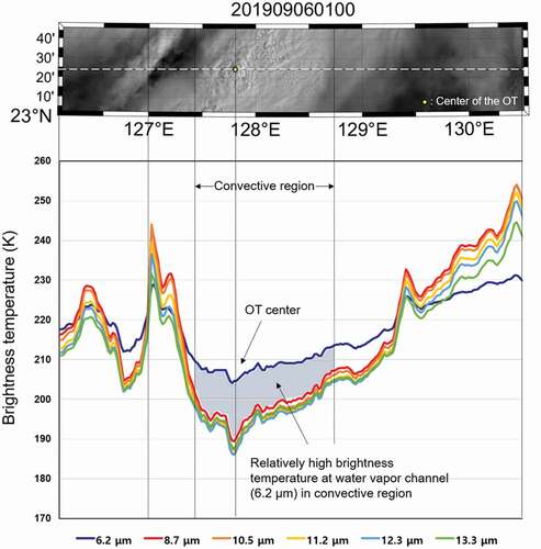
Since OTs are driven by strong updrafts in convective clouds, they have physical characteristics similar to convective clouds. It is revealed that the brightness temperatures at the water vapor infrared channel (5.7–7.1 μm) were 6–8 K higher than the infrared window channel (10.5–12.5 μm) in convective clouds (Schmetz et al. 1997). Figure 1 shows the pattern of brightness temperatures around an OT measured at six-infrared channels that were used in this study. While long-wave infrared channels (10.5, 11.2, 12.4, and 13.3 μm) have similar or higher brightness temperatures than those of the water vapor infrared channel (6.2 μm) over non-convective areas, they show significantly lower values than the water vapor channel in the convective clouds. In addition, there are higher deviations in brightness temperatures of the long-wave infrared channels over weak convective regions than strong convective clouds.

Figure 1. The brightness temperature of six infrared channels around an OT region. The upper figure shows the visible channel-based OT region, and the bottom graph shows the brightness temperature changes by channel. The water vapor infrared channel at 6.2 μm has over 6–8 K higher brightness temperature than the long-wave infrared channels in a convective region. The collection date and time of the scene are expressed as YYYYMMDDhhmn where YYYY is the year, MM is the month, DD is the day, hh is the hour and mm is the minute of the data collection

3. Methodology

3.1. Collecting OT/non-OT samples

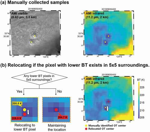
OT and non-OT samples have typically been collected through visual interpretation of relatively high resolution visible images with corresponding infrared data (Bedka et al. 2010). The OT and non-OT samples were collected using GK2A AMI red and long-wave infrared channel data over East Asia from June to November 2019 for training, validation, testing of the proposed approach. Figure 2 shows an example of OT cases collected on 5 September 2019 using GK2A AMI. Since OTs show specific structural characteristics (i.e. dome-like protruding structure with consistent wave-form at visible channels and center-toward brightness temperature descending at infrared channels in isolated regions), we can extract OT reference data in the following ways. First, OT regions that show a dome-shaped structure with surrounding anvil clouds were visually identified from visible channel images (0.64 μm) with high spatial resolution. Subsequently, brightness temperature images at the long-wave infrared wavelength (11.2 μm) were used to check whether the center of the OT regions has much lower brightness temperature than the surrounding anvil clouds. The initially identified center was relocated to a lower brightness temperature region in a 5 × 5 window-buffered area (approximate 20 km x 20 km) when necessary.

Figure 2. Examples of constructing reference data of overshooting tops using the GeoKompsat-2A Advanced Meteorological Imager visible and infrared images collected at 04:00 UTC on 5 September 2019. (a) Collecting OT samples manually based on the spatial characteristics using both channels and (b) relocating the collected samples to the pixel with lower brightness temperature (BT) in 5 × 5 surrounding pixels if necessary. The collection date and time of each scene are expressed as YYYYMMDDhhmn where YYYY is the year, MM is the month, DD is the day, hh is the hour, and mm is the minute of the data collection

We selected distinct OT occurrence cases for training deep learning models (more details in Appendix A). Non-OT samples were randomly collected in the cloud region with no OT, considering various types of clouds (e.g. cirrus, cirrocumulus, and cumulonimbus clouds). A total of 699 OT samples and 7685 non-OT samples for training and validation purposes were collected from 183 scenes from June to September 2019, a season when OTs generally occur in the study area. The collected reference samples were randomly divided into 8:2 for training and validation data, respectively. The validation data were used to optimize the parameters during training the models. Additional six test scenes for both summer (June to August in 2019 and 2020) and autumn (October to November in 2019) seasons were used to evaluate the proposed models. The six scenes were not used for training and therefore completely independent data for accuracy assessment. The 374 cases of OTs are collected for evaluating the scene-based test performances.

3.2. Data augmentation

Data-driven empirical models, including machine learning, have shown various performances depending on the quality and quantity of training data (Yu et al. 2017). In particular, deep learning algorithms have many parameters to be optimized, which require a number of training samples with high quality. Since GK2A AMI is a relatively new satellite sensor, the samples collected from June to September might not be enough to be used as training data. Therefore, we augmented the training data to successfully train the proposed deep learning model.

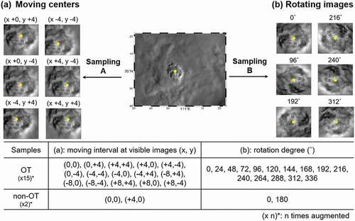
There are several augmentation methods that have been proposed for deep learning applications (Bloice, Stocker, and Holzinger 2017; Frid-Adar et al. 2018; Okafor, Schomaker, and Wiering 2018). We tested two widely used data augmentation methods for image-based deep learning applications (Figure 3): center moving (Sampling A (Kim, Lee, and Im 2018)) and image rotating (Sampling B) based image augmentation. The OT and non-OT samples were augmented fifteen times and twice, respectively. In the sampling A process, the center of the input image of a sample was moved in fourteen-directions (i.e. (x + 0, y + 4), (+4,+4), (+4,0), (+4,-4), (0,-4), (−4,-4), (−4,0), (−4,+4), (−8,+4), (−8,0), (−8,-4), (+8,+4), (+8,0), and (+8,-4)) for OT samples and one-direction (i.e. (x + 4, y + 0)) for non-OTs horizontally and vertically with four-pixel intervals (≒ 2 km) based on visible images. In the sampling B process, the input image of a sample was rotated with a 24-degree interval for OTs and a 180-degree interval for non-OTs. Through this oversampling process, all training samples were augmented from 699 of OTs and 7,685 of non-OTs to 10,485 of OTs and 15,370 of non-OTs

Figure 3. Two types of data augmentation methods. (a) The image augmentation based on the moving approach (Kim, Lee, and Im 2018). The number after “x” means the horizontal moving while the number after “y” indicates the vertical moving of the image center. (b) The image rotation-based augmentation method with maintaining the center of the input image as the center of an OT. OT samples were augmented by fifteen-times and non-OT samples were augmented twice. The collection date and time of the scene are expressed as YYYYMMDDhhmn where YYYY is the year, MM is the month, DD is the day, hh is the hour, and mm is the minute

3.3. Input data preparation

In order to consider both image-based texture recognition and multi-infrared channel-based physical characteristics, the size of input images should be large enough to cover an OT region and the relative differences of brightness temperature among multi-spectral infrared channels should be maintained. Since an OT generally has a diameter less than 15 km (Bedka et al. 2012), we determined the patch size as 31 × 31 in the visible channel (about 15 km × 15 km) and 7 × 7 in the infrared channels (about 14 km x 14 km). In addition, six-infrared channels were stacked and spatially normalized with a min-max approach for preserving the deviations of brightness temperatures among the infrared channels. After chopping 31 × 31 sized images of the visible channel data and 7 × 7 sized images of infrared channel data based on OT/non-OT samples, three-types of input datasets were constructed (Figure 4): 1) Input set 1 consists of 31×31-pixel visible channel images and downscaled 31 × 31 single infrared window channel (11.2 μm) images which was proposed in Kim, Lee, and Im (2018), 2) Input set 2 consists two groups of the input images, one with single visible images and the other with six-banded infrared images (i.e. 6.2, 8.6, 10.4, 11.2, 12.4, and 13.3 μm), and 3) Input set 3 consists two groups of input images, one with single-banded visible images and the other with two-banded infrared images (i.e. 6.2 and 11.2 μm). While the six-banded infrared channels in Input set 2 are widely used for detecting convective cloud region (Bedka et al. 2012; Setvák et al. 2013; Bedka and Khlopenkov 2016; Kim et al. 2017; Han et al. 2015), the two-banded infrared channels in Input set 3 include the infrared window channel and the water vapor channel which have independent characteristics over the OT surrounding regions.

Figure 4. Three types of input data. Input set 1 consists of visible images (0.64 μm) with a 31 × 31 pixel window and the downscaled long wave infrared images (11.2 μm) with the same window size. Input set 2 consists of visible images with a 31 × 31 pixel window and all six infrared images with a 7 × 7 pixel window. Input set 3 consists of visible images with a 31 × 31 window, and two infrared (6.2 and 11.2 μm) images with a 7 × 7 window. The collection date and time of the scene are expressed as YYYYMMDDhhmn where YYYY is the year, MM is the month, DD is the day, hh is the hour, and mm is the minute

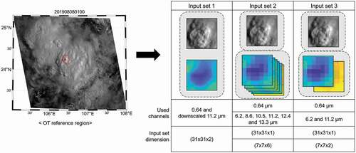
While the infrared channel images in Input set 1 were downscaled to 0.5 km for stacking with high-resolution visible images using bicubic resampling, Input sets 2 and 3 preserved the original resolution of the infrared channels, which can effectively reduce the computing cost for training multi-infrared channel images.

3.4. Feature aggregated deep learning with convolutional neural networks (CNNs)

CNNs are one of the state-of-the-art deep learning algorithms for pattern recognition. The hierarchical networks of CNNs that consist of convolutional layers, pooling layers, and fully connected layer(s) extract feature vectors from multi-dimensional input data. Therefore, they have been widely used for recognizing not only 2-dimensional images (e.g. animal photos, hand writing numbers, and satellite images) but also 3-dimensional structures such as a structure magnetic resonance imaging (MRI) of the brain, human action recognition (LeCun et al. 1989; Ji et al. 2012; Sothe et al. 2020). Remote sensing data have been analyzed using CNNs for monitoring environments or human activities (Ao et al. 2019; Yang et al. 2019; Duarte et al. 2020; Park et al. 2019; Zhao et al. 2020; Ahishali et al. 2021). Furthermore, CNNs have been used in the atmospheric and climate domains such as predicting El-Nino by analyzing numerical model-based image patterns and estimating tropical cyclone intensity by recognizing satellite-based images (Kim, Lee, and Im 2018; Pradhan et al. 2017; Ham, Kim, and Luo 2019; Lee et al. 2020a, 2020b).

Convolutional layers are the most essential part of CNNs. The dot-product operation between the moving window and the given images is conducted to find the hidden features. These filters are randomly initiated and tuned during the training. Finally, each filter can represent the specific feature of the dataset. In pooling layers, the size of the image is reduced to extract the local representative values such as the maximum or average from sub-windows. Pooling operation can bring multiple advantages, including the robustness from the noise, the invariance to scale difference (Boureau et al. 2010), and the significantly reduced computational cost. The convolutional and pooling layers conduct the spatial feature extraction, keeping the spatial information from the original images. In the fully connected layer, this information is converted into 1-D vectors to conduct classification. The stacking of the non-linear activation functions is done to make CNNs non-linear. The rectified linear unit (ReLU) is typically used as the activation function in the convolutional and fully connected layers. ReLU can simply make the network non-linear with the identity function and zero (Nair and Hinton 2010). As ReLU returns zero with negative input values, weights cannot be updated during the training once converted into zero, which is called the dying ReLU problem. Leaky ReLU can mitigate this problem returning a linear function with a small slope (i.e. $\alpha$; typically 0.1–0.01) at the negative input range (Maas, Hannun, and Ng 2013). Both ReLU and Leaky ReLU were used in our models as activation functions (Table 2).

Table 2. Architectures of the three models. C means convolutional layer, P means pooling layer, H means hidden layer and D means drop out. The number(*number) after @ means horizontal (*depth) size of filter. The following numbers after C, P, and H mean the filter number of the convolutional layers, the size of the pooling layers, and the hidden node of the fully connected layer, respectively. In all models, the first convolutional layer was activated with the “Leaky ReLU” function with an $\alpha$ of 0.01 and the others were activated with the “ReLU” function. The models classify whether each input is OT or not

Model architecture	Input structure (height * width * depth)	Convolutional networks		Fully connected layer	Output
		CNN type	Architecture of CNNs
Model 1 (w/ Input set 1)	(31 * 31 * 2)	2D	C32@3, C32@3, P2, D0.25, C64@3, C64@3, P2, D0.25	H1024, H256	OT/ NonOT
Model 2 (w/ Input set 2)	(31 * 31 * 1)	2D	C64@5, P2, D0.25, C128@3, P2, C272@3, D0.25	H512, H128
	(7 * 7 * 6)	2D	C64@3, D0.25, C128@2, P2, C192@2, D0.25
Model 3 (w/ Input set 3)	(31 * 31 * 1)	2D	C64@5, P2, D0.25, C128@3, P2, C272@3, D0.25	H192, H64
	(7 * 7 * 2)	3D	C64@3*1, C128@2*1, C192@2*1, D0.25

A softmax classifier, cross-entropy fuction, and adam optimization were used in the proposed CNN models. The softmax classifier takes the output of the last fully connected layer and calculates the normalized probability of every class (Dunne and Campbell 1997). Finally, the class with maximum probability is assigned to the estimated result of the model. The cross-entropy loss can compute the loss between the estimated value and reference value using the probability vector from the softmax function. When the loss is calculated, the optimization process is conducted to minimize the loss value by the iterative approach. Adaptive moment estimation (Adam) optimization has been widely used, showing good performance and fast convergence compared to other methods (Kingma and Ba 2014).

While CNNs have the strength in analyzing image data, input data should have the same spatial resolution. To mitigate this limitation, a feature aggregation deep learning approach was proposed for learning multi-level and multi-scale input datasets (Lee and Nam 2017). The multi-scaled datasets were pre-trained through multiple neural networks, and the extracted features were aggregated to be used as input data for the post-deep learning process. The feature aggregated deep learning-based model proposed in Lee and Nam (2017) allows to preserve the original structures of input data and makes the model more efficient. Since the image data used in the present study have different spatial resolutions (i.e. 0.5 km for VIS and 2 km for IRs), we adopted the CNN-based pre-trained feature aggregate deep learning approach for developing OT discriminative model with an efficient use of the multi-dimensional input data.

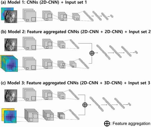
In this study, we compared three-types of deep learning-based OT detection models including one approach proposed in Kim, Lee, and Im (2018). Figure 5 and Table 2 summarize the architectures of the three models according to the types of input data. The hyper-parameters, such as kernel number, kernel size, pooling size, drop-out rate, and layer depth, were fixed through a grid-search method, and finally we identified the relatively optimized architecture for each input set. The input dataset applied to each model architecture was selected through pre-optimization training results according to computational efficiency and classification performance. While model 1 is a typical two-dimensional CNN (2D-CNN) with input set 1, model 2 and model 3 are feature aggregated deep learning with multi-dimensional CNNs based on input set 2 and input set 3, which consist of two types of input data with different horizontal dimensions (i.e. 31 × 31 for VIS images and 7 × 7 for IR images). While model 2 consists of two 2D-CNN algorithms, model 3 consists of one 2D-CNN and one 3D-CNN algorithms. While 2D-CNNs have two-dimensional kernels in the convolutional layers, 3D-CNNs have three-dimensional kernels in the convolutional layers. When passing the convolutional layers, the output is calculated with the sum of the dotted product between inputs and kernels. Therefore, while 2D-CNNs merge the features from multi-layers of an input dataset, 3D-CNNs could preserve the layered features. The details of the model architecture with hyper-parameters are described in Table 2.

Figure 5. Three types of deep learning architectures used in this study. (a) model 1: The 2D-CNN architecture using input set 1, (b) model 2: The feature-aggregated deep learning model consisting of two 2D-CNN models using input set 2, and (c) model 3: The feature-aggregated deep learning model consisting of 2D-CNN and 3D-CNN in parallel using input set 3.

The three types of models (i.e. model 1, model 2, and model 3) were constructed using two types of augmented input datasets (i.e. sampling A and sampling B). According to the sampling method and model architecture, we tested six schemes: scheme A1: model 1 with sampling A, scheme A2: model 2 with sampling A, scheme A3: model 3 with sampling A, scheme B1: model 1 with sampling B, scheme B2: model 2 with sampling B, and scheme B3: model 3 with sampling B. Scheme A1 is modeled on the architecture proposed in the previous study (Kim, Lee, and Im 2018), serving as a control model. The schemes are summarized in Table 3.

Table 3. Schemes according to sampling methods and model architectures

Scheme	Sampling method	Model architecture
A1 (Kim, Lee, and Im 2018)	Sampling A (Center moving)	Model 1
A2		Model 2
A3		Model 3
B1	Sampling B (Image rotation)	Model 1
B2		Model 2
B3		Model 3

3.5. Accuracy assessment

The constructed models were evaluated using six test scenes (i.e. 29 July 2019 00:00 UTC, 2 August 2019 01:00 UTC, 9 October 2019 01:00 UTC, 6 November 2019 02:00 UTC, 5 June 2020 02:00 UTC and 5 August 2020 00:00 UTC over the East Asia region observed by GK2A AMI), which were not used for training the models. To evaluate the performance of the proposed deep learning models, three statistical metrics were used: the probability of detection (POD), the false alarm rate (FAR), and the critical success index (CSI).

(1) $POD=\frac{A}{\left(A+B\right)}\ast 100$(1)

(2) $FAR=\frac{C}{\left(A+C\right)}\ast 100$(2)

(3) $CSI=\frac{A}{\left(A+B+C\right)}$(3)

where A is the number of correctly detected cases, B represents the number of not-detected but observed cases, and C means the number of falsely detected cases. POD shows how well the model detected the targets while FAR represents how falsely the model performed. The CSI is an index to indicate the general performance of the classification model considering both POD and FAR. The POD and FAR values range from 0% to 100%, which means that the higher the POD and the lower the FAR, the better performance of the model. The CSI ranges from 0 to 1, and the closer to 1, the higher model accuracy. In this study, the CSI index was mainly used to judge the overall performances and to compare the six schemes (i.e. schemes A1, A2, A3, B1, B2, and B3).

Since OTs are a part of the atmospheric convective processes, the difference between WV (6.2 μm) and IRW (11.2 μm) brightness temperatures can be used to present the convective level (Schmetz et al. 1997; Ai et al. 2017). By classifying the difference using specific thresholds, we zoned the regions according to the convection level (Han et al. 2015; Schmetz et al. 1997): The region where the difference is over 6 is considered as an “extreme convection” region, between 3 and 6 corresponds to “strong convection,” between 0 and 3 is considered as “moderate convection,” and between −5 and 0 corresponds to “weak convection.” Here, we proposed the ratio of false alarms to correctly detected OTs (hereafter FCR) according to the level of convective clouds. It was used to identify how the model performance changed depending on the levels of convection. The ratio is calculated as:

(4) $FCR=\frac{\mathrm{\#}\hspace{0.17em}of\hspace{0.17em}faslsely\hspace{0.17em}detected\hspace{0.17em}OTs}{\mathrm{\#}\hspace{0.17em}of\hspace{0.17em}correctly\hspace{0.17em}detected\hspace{0.17em}OTs}$(4)

A low FCR value implies that the model well classifies the OT and non-OT regions. On the other hand, a high FCR value at a specific convective level indicates that the model has poor performance with a high false alarm ratio compared to the OT occurrence rate at the region.

4. Results and discussion

4.1. Overshooting tops classification results

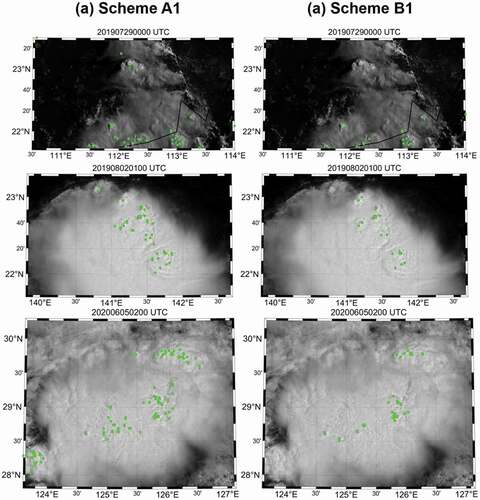
Figure 6 shows the evaluation results of six schemes using six test scenes, and Table 4 summarizes the overall performance of each scheme. Among all schemes, the sampling B method (i.e. schemes B1, B2 and B3) resulted in significantly improved CSI scores than the sampling A method (i.e. schemes A1, A2, and A3). While the sampling B-based models showed the PODs similar to the sampling A-based models, they resulted in a significant improvement in terms of FAR, up to 20.3%, 29.0%, and 40.6% of reduction in schemes B1, B2, and B3, respectively. Figure 7 shows the OT detection results by schemes A1 and B1. While scheme B1 tended to detect the center pixels of OTs relatively well, scheme A1 often resulted in the over-estimation of OT regions including non-convective areas (e.g. cirrus and edge of the cloud).

Table 4. Overall performance of the OT detection models by scheme using the six test scenes. The best results are shown in bold

Scheme	POD (%)	FAR (%)	CSI
Scheme A1 (Kim, Lee, and Im 2018)	87.3	50.9	0.3
Scheme A2	86.8	64.2	0.3
Scheme A3	88.9	49.9	0.4
Scheme B1	90.6	41.4	0.4
Scheme B2	86.4	45.5	0.4
Scheme B3	92.1	21.5	0.7

Figure 6. Test results by scheme (i.e. schemes A1, A2 A3, B1, B2 and B3) using six test scenes collected in the summer (i.e. 29 July 2019 00:00 UTC, 2 August 2019 01:00 UTC, 5 June 2020 02:00 UTC and 5 August 2020 00:00 UTC) and autumn seasons (i.e. 9 October 2019 01:00 UTC and 6 November 2019 02:00 UTC) in 2019 and 2020. The collection date and time of each test scene are expressed as YYYYMMDDhhmn; YYYY is the year, MM is the month, DD is the day, hh is the hour, and mm is the minute of the data collection

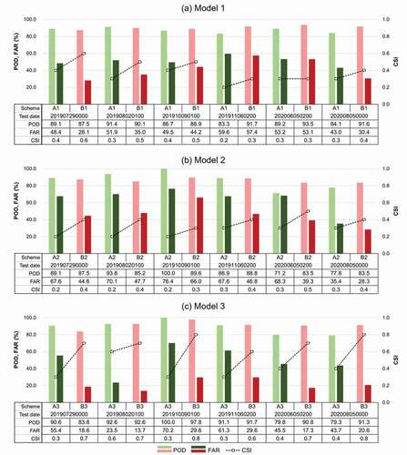
Figure 7. OT detection results of schemes A1 and B1 using the images collected on 29 July 2019 00:00 UTC, 2 August 2019 01:00 UTC and 5 June 2020 02:00 UTC. Green dots show the OTs detected by each scheme. The collection date and time of each scene are expressed as YYYYMMDDhhmn where YYYY is the year, MM is the month, DD is the day, hh is the hour, and mm is the minute of the data collection

Model performance varied by model architecture. For both sampling approaches, model 3 (i.e. schemes A3 and B3) showed the best performance while model 2 (i.e. schemes A2 and B2) yielded the worst. Although models 2 and 3 have a similar neural network architecture with pre-trained feature aggregated deep learning, they showed a large difference in their performance especially in terms of FAR. While model 2 was trained based on one visible and six-infrared images (i.e. 6.2, 8.7, 10.5, 11.2, 12.3, and 13.3 μm), model 3 was trained with one visible and two-infrared channels (i.e. 6.2 and 11.2 μm). We tested 2D-CNNs and 3D-CNNs in models 2 and 3 for analyzing the six-infrared images and two-infrared images to find out the contribution of the architectures for model performance. When testing with the six-infrared channel images, the 2D-CNNs based model showed slightly higher or similar performance than the 3D-CNNs based model. On the other hand, when testing with the two-infrared channel images, the 3D-CNNs based model resulted in significantly high performance than the 2D-CNNs based model. As mentioned in section 2.1, the infrared channels excluding water vapor (6.2 μm) show similar trends around real-OT regions, which may induce confusion on training the parameters of the CNN-based model. On the other hand, model 3 could focus on the salient information to configure convective cloud based on the differences of WV and IRW channel data, which could effectively train both spatial and physical characteristics OTs such as convective levels. In addition, the three-dimensional kernels of 3D-CNNs helped considering the distinct infrared channels independently without any merging process. Figure 8 shows the monitoring results according to three types of deep learning architectures with image rotating pre-processing (i.e. sampling B). Through the evaluation of the models, scheme B3 resulted in the best performance especially in terms of FAR. When compared to scheme A1, the architecture proposed by previous study (Kim, Lee, and Im 2018), the POD slightly increased by 4.8% from 87.3% to 92.1%, FAR decreased by about 29% from 50.9% to 21.5%.

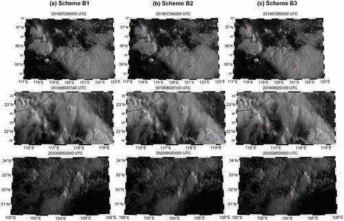
Figure 8. OT detection results using the images collected on 29 July 2019 00:00 UTC, 2 August 2019 01:00 UTC and 5 August 2020 00:00 UTC. The dot marks colored with green, blue and red represent the detection results by schemes B1, B2 and B3, respectively. The collection date and time of each scene are expressed as YYYYMMDDhhmn where YYYY is the year, MM is the month, DD is the day, hh is the hour, and mm is the minute of the data collection

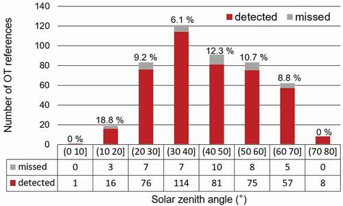
4.2. Validation according to solar zenith angles

Solar zenith angle (SZA) is the angle between a perpendicular line to the Earth’s ground and sun rays. The spatial characteristics of OTs such as OT-induced shadows at visible channels change depending on the angel of the sun (Bedka and Khlopenkov 2016). Therefore, it is necessary to verify the detection performances according to SZAs. Figure 9 shows the scheme B3 model performance for the OT references using the test scenes in summer (i.e. 29 July 2019 00:00 UTC, 2 August 2019 01:00 UTC and 5 June 2020 02:00 UTC, 5 August 2020 00:00 UTC). Over 80% of OTs occurred in the region with SZAs from 20 to 60 degrees, and the model achieved a detection rate of 91.5%. The model produced a detection rate of 93.3% for SZAs with less than 20 degrees and more than 60 degrees. Overall, the model performance did not show a notable bias depending on SZAs, which implies that our CNN-based model shows robust detection performance according to SZAs.

Figure 9. The number of OT occurrences detected and missed using scheme B3 in the summer (i.e. 29 July 2019 01:00 UTC, 2 August 2019 01:00 UTC, 5 June 2020 02:00 UTC and 5 August 2020 00:00 UTC) according to solar zenith angles (SZAs)

4.3. Consecutive monitoring of overshooting tops

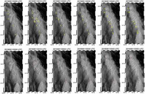
The continuous detection of OTs is also possible when using geostationary satellite data with high temporal resolution (e.g. 10 min). Figure 10 shows the scheme B3-based hourly OT monitoring results on 23 July 2020. All hourly day time scenes (i.e. from 21:00 UTC to 11:00 UTC in summer over East Asia) were used for evaluating the monitoring performance. On average, the model resulted in a POD of 92.4%, FAR of 15.7%, and CSI of 0.8, which were consistent with the scheme B3 results shown in Figure 6 and Table 4. It indicates that our CNN-based model can be used for the operational monitoring of OTs. Figure 11 shows consecutive scenes at a 10-min interval from 11 August 2019, 00:00 UTC to 00:50 UTC and Table 5 summarizes the consecutive monitoring results during this period. There were thirteen OT cases from occurrence to disappearance in this region over the course of 1 hour. The ‘Case 1ʹ was generated around 00:00 UTC and disappeared between 00:10 and 00:20 UTC with the shortest lifetime among the thirteen cases. Since the ‘Case 1ʹ was in the early generation stage at 00:00 UTC, the proposed model did not detect the region as an OT. Similarly, the ‘Case 13ʹ at 00:40 UTC was also in the early stage, our model was not able to identify the spatial characteristics of typical OTs. On the other hand, the “Case 7,” which was generated between 00:00 and 00:10 UTC and disappeared around 00:40 UTC, had relatively low detection performance in the extinction stage. About 70% of the OT cases (9 cases among 13 cases) shows 100% of detection probability in this period. Since the OTs in the early generation and extinction phases do not always have the typical structural characteristics of OTs, such as a dome-like protrusion structure with surrounding anvil clouds, it is often difficult to classify them as OTs.

Table 5. Consecutive monitoring results of the 13 OT cases from 11 August 2019 00:00 UTC to 05:00 UTC. While the gray shading indicates the occurrence period of each OT, “O” and “X” represent the case detected and missed by the model (scheme B3), respectively. The case numbers correspond to the OT identification numbers in Fig. 11

Time (UTC)	11/08/2019						Probability of detection in this period
	00:00	00:10	00:20	00:30	00:40	00:50
Case 1	X	O					50%
Case 2	O	O	O	O			100%
Case 3	O	O	O				100%
Case 4	O	O	O	O			100%
Case 5	O	O	O	O	O	O	100%
Case 6		O	O	O			100%
Case 7		O	O	X	X		50%
Case 8				X	O		50%
Case 9					O	O	100%
Case 10					O	O	100%
Case 11					O	O	100%
Case 12					O	O	100%
Case 13					X	O	50%

Figure 10. Hourly validation results based on the scenes of 23 July 2020 using scheme B3. The detecting performances were evaluated using POD, FAR and CSI indices. Since the visible channel images were not available at nighttime (i.e. 12:00 to 20:00 UTC in summer over East Asia), hourly observations during 00:00 UTC – 11:00 UTC and 21:00 UTC – 23:00 UTC were used

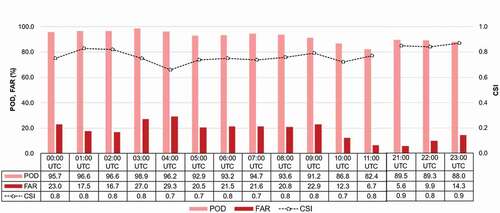
Figure 11. Monitoring the lifetime of OTs with a 10-minute interval on 11 August 2019 from 00:00 UTC to 00:50 UTC. The top images show reference OTs identified from the period in yellow, while the bottom images show the OTs detected by scheme B3 in magenta. During this period, a total of 13 OTs (numbered in the top images) were observed in this region. OTs with both number and alphabet mean that they were generated from the same updraft system (i.e. ‘5ʹ, “5a” and “5b”) or merged to the same updraft system (i.e. “6a,” “6b,” “6 c” and ‘6ʹ). The collection date and time of each scene are expressed as YYYYMMDDhhmn where YYYY is the year, MM is the month, DD is the day, hh is the hour, and mm is the minute of the data collection

4.4. Visualization of the deep learning-based OT detection model

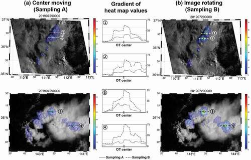
As the interest of deep learning has increased in the meteorological domain, many deep learning-based studies have been conducted (Deo and Şahin 2015; Tebbi and Haddad 2016; Liu et al. 2016; Lagerquist, McGovern, and Gagne II 2019; McGovern et al. 2019). However, since deep learning-based models have been regarded as “black box” models, it is difficult to interpret the influence of input variables on OT detection. In order to overcome such a limitation, several visualization methods have been proposed in previous research (Simonyan, Vedaldi, and Zisserman 2013; Zhou et al. 2016; Selvaraju et al. 2017; Li and Itti 2010). A class activation mapping (CAM) is a widely used visualizing method for CNNs-based models. It enables to analyze which regions of input images have contributed more to classification (Zhou et al. 2016). A CAM can be extracted as the sum of the last feature maps of convolutional layers, and a so-called heat map is created to show the regions on which the model is focused while training. The CAM-based visualizing method has been used for understanding the CNN based model and it shows reasonable results in meteorological domain (Miller et al. 2018; Ham, Kim, and Luo 2019; Lee et al. 2020a).

Figure 12 shows the heat maps based on schemes A3 and B3. While there were relatively low deviations of heat map values between the OT center and surrounding pixels in the sampling A-based model results, OT centers were more clearly highlighted in the sampling B-based model results. It means that the sampling A-based model is likely to fail to distinguish OTs from non-OT regions. Sampling A could induce an increase in the proportion of the surroundings of OTs within input images as it shifts the center of OTs. Thus, the method might blur the information of the center of OTs with surrounding areas, less focusing on the center of OTs, resulting in misclassification. On the other hand, as sampling B keeps the center position of OTs located at the center of the input images, the steeper up-gradient of the heat map values were found toward the OT centers, which then better distinguished the dome-like OT center patterns from the surrounding pixels than the sampling A-based models.

Figure 12. Heat maps based on schemes A3 (a) and B3 (b). The blue to red color scheme shows the attention level by the deep learning models: The more reddish, the more attention. The scheme B3’s heat map shows a much steeper gradient toward the OT centers than the scheme A3’s ones. The date and time of each scene are expressed as YYYYMMDDhhmn where YYYY is the year, MM is the month, DD is the day, hh is the hour and mm is the minutes of the data collection

4.5. Test results according to the convection level

To examine the detection performance according to the four convection levels (i.e. extreme, strong, moderate, and weak convections), the six test scenes were used. Figure 13a shows the convection ratios determined based on the differences in the brightness temperatures between WV and IRW. Figure 13b illustrates the FCR (Eq. (4(4) $FCR=\frac{\mathrm{\#}\hspace{0.17em}of\hspace{0.17em}faslsely\hspace{0.17em}detected\hspace{0.17em}OTs}{\mathrm{\#}\hspace{0.17em}of\hspace{0.17em}correctly\hspace{0.17em}detected\hspace{0.17em}OTs}$(4) )) as a function of the convective level for schemes B1, B2, and B3 in the summer and autumn seasons. Because the three models yielded similar PODs, we compared the FCR for the four convection phases. To verify the seasonality of the performance, we divided the six test scenes into summer (i.e. 29 July 2019 00:00 UTC, 2 August 2019 01:00 UTC, 5 June 2020 02:00 UTC and 5 August 2020 00:00 UTC) and autumn cases (i.e. 6 October 2019 01:00 UTC and 9 November 2019 02:00 UTC).

Figure 13. (a) The convective level classification using the difference of brightness temperature (BTD) between water vapor (WV) and infrared window (IRW) channels. The region with difference of WV and IRW over 6 is defined as “Extreme convection,” between 3 to 6 is defined as “Strong convection,” between 0 to 3 is defined as “Moderate convection” and between −5 to 0 is considered as “Weak convection.” (b) The FCRs (falsely to correctly detected ratio) of OTs by the convective level and scheme (i.e. Scheme B1, B2 and B3)

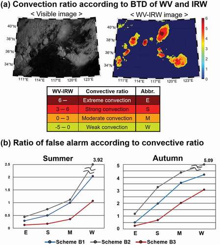
Overall, the stronger the convection, the lower the FCR for both seasons in all schemes. When compared to schemes B1 and B2, the FCR of scheme B3 showed the lowest value in all convective levels. It implies that the relative convective level that can be extracted from the difference of WV and IRW and the spatial distribution of water vapor that can be extracted from VIS and IRW play an important role in OT detection. Scheme B3 provided the most robust performance in both seasons among the schemes, which implies the potential use of the proposed model for other seasons. Meanwhile, scheme B2 produced higher FCR values in all convective levels, which is consistent with the scene-based evaluation results (see Figure 6), showing especially high FCR in weak convective regions. It means that most of the false alarms from scheme B2 occurred in weak convective regions.

The differences in FCRs were generally larger in autumn than in summer. Since extreme convection mostly occurs in summer over East Asia (Latrach 2013; Xian and Fu 2015; Punge et al. 2017), the training data were collected during the summer season. It might result in somewhat degraded performance in autumn. Nevertheless, scheme B3 has a discriminative ability of simultaneously considering WV and IRW, which helps the model mitigate the seasonality of the performance. Note that the use of IRW data only for OT detection can be sensitive to seasons.

4.6. Overshooting top detection at nighttime

Since OTs can be identified based on their dome-like protrusion shape in the visible channel and the center-focused gradient of brightness temperature in IR channels, most studies for OT detection have used both visible and IR data (e.g. Bedka and Khlopenkov 2016; Setvák et al. 2013; Kim, Lee, and Im 2018). However, the visible channel cannot be used at night and dawn (11:00 UTC – 22:00 UTC in June-July-August over East Asia). In order to evaluate the performance of the proposed model (scheme B3 with the best performance) at certain times, we additionally tested the model without using the visible image. The model was trained using two IR channels (i.e. 6.2 and 11.2 μm) with the same architecture of scheme B3. The nighttime model was then applied to two scenes collected at night (i.e. 29 July 2019 20:00 UTC and 8 August 2019 20:00 UTC).

Figure 14 shows the test results of the model trained without visible images for two scenes at nighttime (i.e. 29 July 2019 20:00 UTC and 8 August 2019 20:00 UTC). Although it is hard to identify OT regions from IR images with high confidence, we can still use the gradient descent of brightness temperatures from the surrounding areas to define OT reference regions. In general, the OT-like regions were correctly detected as OTs, as shown in red-dashed circles in the right-hand panel of Figure 14.

Figure 14. The test results of 29 July 2019 20:00 UTC and 8 August 2019 20:00 UTC using the model trained without the visible channel. The background images are derived from IRW (11.2 μm) channel with brightness temperature (BT). The yellow dots indicate detection results from the model. The right figures are the zoomed-in images of the white-lined boxes in the left figures. The dashed red circles in the right figures indicate OT candidate regions with high confidence. The date and time of each scene are expressed as YYYYMMDDhhmn where YYYY is the year, MM is the month, DD is the day, hh is the hour, and mm is the minute of the data collection

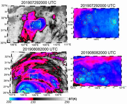
It was found that non-OT-like regions, with no local gradient descending of brightness temperatures over strong convective regions, especially a typhoon eyewall on 8 August 2019 20:00 UTC (lower left in the left-hand panel of Figure 14), were misclassified as OTs. This may be because the model mainly focused on the water vapor contents with convective levels as well as the spatial distribution of water vapor with coarse resolution. Such misclassified areas might have correctly detected when the information from visible images of high spatial resolution was incorporated. Although the nighttime model tended to result in more false alarms when compared to the model with VIS images, it still showed the potential of OT monitoring at nighttime.

5. Conclusion

In this research, we proposed a deep learning-based OT detection model using multi-channel data from GK2A AMI. Six schemes considering two data augmentation approaches and three deep learning architectures were investigated to determine the optimum model for OT detection and monitoring over East Asia. The results showed that scheme B3 produced the best performance with a POD of 92.1%, a FAR of 21.5%, and a CSI of 0.7. When compared to the previous deep learning model (scheme A1), the POD increased by 4.8% and FAR decreased by 29.4%. Image rotation-based data augmentation (sampling B) performed better than the center-moving method (sampling A) regardless of the deep learning architectures based on the model performance and heat map analysis. Both water vapor and infrared data were very useful to detect OTs, but not all six infrared channels were necessary for OT detection. The consecutive monitoring of the OT cases was also investigated using time-series images with the 10-minute interval. While 9 cases out of the 13 (~70%) were correctly detected during the one hour of the experiment, four cases at early generation or extinction phases were missed.

While the proposed model produced promising results, there are still some limitations, which should be improved in further research: 1) it is hard to estimate stage of OTs using binary classification. More training data at early OT generation and extinction phases can further improve the consecutive monitoring of OTs; 2) the proposed model tends to over-detect OTs especially in the strong convective areas at nighttime. A nighttime model based only on infrared channels can improve the operational monitoring of OTs, although it is difficult to evaluate the models using reference data at night. Downscaling of infrared channels might improve the performance of OT detection at nighttime; and 3) although various combinations of model architecture were evaluated, they were not fully optimized. We should examine more diverse model architectures especially when 3D-CNNs are used with much more hyper-parameters to be optimized than 2D-CNNs.

Disclosure statement

No potential conflict of interest was reported by the authors.

Supplementary material

Supplemental data for this article can be accessed here.

Correction Statement

This article has been republished with minor changes. These changes do not impact the academic content of the article.

Additional information

Funding

This work was supported by the Ministry of Science and ICT (MSIT), South Korea (IITP-2021-2018-0-01424), and a grant (no. 20009742) of Ministry-Cooperation R&D program of Disaster-Safety, funded by Ministry of Interior and Safety (MOIS), South Korea. J. Lee is partially supported by Basic Science Research Program through the National Research Foundation of Korea (NRF) funded by the Ministry of Education of South Korea (no. 2020R1A6A3A13077532).

References

- Ahishali, M., S. Kiranyaz, T. Ince, and M. Gabbouj. 2021. “Classification of Polarimetric SAR Images Using Compact Convolutional Neural Networks.” GIScience & Remote Sensing 58 (1): 28–47. doi:https://doi.org/10.1080/15481603.2020.1853948.
- Ai, Y., J. Li, W. Shi, T. J. Schmit, C. Cao, and W. Li. 2017. “Deep Convective Cloud Characterizations from Both Broadband Imager and Hyperspectral Infrared Sounder Measurements.” Journal of Geophysical Research: Atmospheres 122 (3): 1700–1712.
- Ao, W., Y. Fu, X. Hou, and F. Xu. 2019. “Needles in a Haystack: Tracking City-scale Moving Vehicles from Continuously Moving Satellite.” IEEE Transactions on Image Processing 29: 1944–1957. doi:https://doi.org/10.1109/TIP.2019.2944097.
- Bedka, K., J. Brunner, R. Dworak, W. Feltz, J. Otkin, and T. Greenwald. 2010. “Objective Satellite-based Detection of Overshooting Tops Using Infrared Window Channel Brightness Temperature Gradients.” Journal of Applied Meteorology and Climatology 49 (2): 181–202. doi:https://doi.org/10.1175/2009JAMC2286.1.
- Bedka, K. M. 2011. “Overshooting Cloud Top Detections Using MSG SEVIRI Infrared Brightness Temperatures and Their Relationship to Severe Weather over Europe.” Atmospheric Research 99 (2): 175–189. doi:https://doi.org/10.1016/j.atmosres.2010.10.001.
- Bedka, K. M., R. Dworak, J. Brunner, and W. Feltz. 2012. “Validation of Satellite-based Objective Overshooting Cloud-top Detection Methods Using CloudSat Cloud Profiling Radar Observations.” Journal of Applied Meteorology and Climatology 51 (10): 1811–1822. doi:https://doi.org/10.1175/JAMC-D-11-0131.1.
- Bedka, K. M., and K. Khlopenkov. 2016. “A Probabilistic Multispectral Pattern Recognition Method for Detection of Overshooting Cloud Tops Using Passive Satellite Imager Observations.” Journal of Applied Meteorology and Climatology 55 (9): 1983–2005. doi:https://doi.org/10.1175/JAMC-D-15-0249.1.
- Bloice, M. D., C. Stocker, and A. Holzinger. 2017. “Augmentor: An Image Augmentation Library for Machine Learning.” Journal of Open Source Software 2(19), 432. doi:https://doi.org/10.21105/joss.00432.
- Boureau, Y. L., F. Bach, Y. LeCun, and J. Ponce. 2010, June. Learning Mid-level Features for Recognition.Paper presented at the 2010 IEEE computer society conference on computer vision and pattern recognition (pp. 2559–2566). IEEE, San Francisco, June 13-18.
- Chen, C., Y. Li, W. Liu, and J. Huang. 2015. “SIRF: Simultaneous Satellite Image Registration and Fusion in a Unified Framework.” IEEE Transactions on Image Processing 24 (11): 4213–4224. doi:https://doi.org/10.1109/TIP.2015.2456415.
- Deo, R. C., and M. Şahin. 2015. “Application of the Artificial Neural Network Model for Prediction of Monthly Standardized Precipitation and Evapotranspiration Index Using Hydrometeorological Parameters and Climate Indices in Eastern Australia.” Atmospheric Research 161: 65–81. doi:https://doi.org/10.1016/j.atmosres.2015.03.018.
- Dessler, A. E., M. R. Schoeberl, T. Wang, S. M. Davis, and K. H. Rosenlof. 2013. “Stratospheric Water Vapor Feedback.” Proceedings of the National Academy of Sciences 110 (45): 18087–18091. doi:https://doi.org/10.1073/pnas.1310344110.
- Duarte, D., F. Nex, N. Kerle, and G. Vosselman. 2020. “Detection of Seismic Façade Damages with Multi-temporal Oblique Aerial Imagery.” GIScience & Remote Sensing 57 (5): 670–686. doi:https://doi.org/10.1080/15481603.2020.1768768.
- Dunne, R. A., and N. A. Campbell 1997, June. On the Pairing of the Softmax Activation and Cross-entropy Penalty Functions and the Derivation of the Softmax Activation Function. In Proc. 8th Aust. Conf. on the Neural Networks, Melbourne: Citeseer, 181, 185.
- Dworak, R., K. Bedka, J. Brunner, and W. Feltz. 2012. “Comparison between GOES-12 Overshooting-top Detections, WSR-88D Radar Reflectivity, and Severe Storm Reports.” Weather and Forecasting 27 (3): 684–699. doi:https://doi.org/10.1175/WAF-D-11-00070.1.
- Frid-Adar, M., I. Diamant, E. Klang, M. Amitai, J. Goldberger, and H. Greenspan. 2018. “GAN-based Synthetic Medical Image Augmentation for Increased CNN Performance in Liver Lesion Classification.” Neurocomputing 321: 321–331. doi:https://doi.org/10.1016/j.neucom.2018.09.013.
- Fultz, A. J., and W. S. Ashley. 2016. “Fatal Weather-related General Aviation Accidents in the United States.” Physical Geography 37 (5): 291–312. doi:https://doi.org/10.1080/02723646.2016.1211854.
- Ham, Y. G., J. H. Kim, and J. J. Luo. 2019. “Deep Learning for Multi-year ENSO Forecasts.” Nature 573 (7775): 568–572. doi:https://doi.org/10.1038/s41586-019-1559-7.
- Han, H., S. Lee, J. Im, M. Kim, M. I. Lee, M. H. Ahn, and S. R. Chung. 2015. “Detection of Convective Initiation Using Meteorological Imager Onboard Communication, Ocean, and Meteorological Satellite Based on Machine Learning Approaches.” Remote Sensing 7 (7): 9184–9204. doi:https://doi.org/10.3390/rs70709184.
- Holton, J. R., P. H. Haynes, M. E. McIntyre, A. R. Douglass, R. B. Rood, and L. Pfister. 1995. “Stratosphere‐troposphere Exchange.” Reviews of Geophysics 33 (4): 403–439. doi:https://doi.org/10.1029/95RG02097.
- Ji, S., W. Xu, M. Yang, and K. Yu. 2012. “3D Convolutional Neural Networks for Human Action Recognition.” IEEE Transactions on Pattern Analysis and Machine Intelligence 35 (1): 221–231. doi:https://doi.org/10.1109/TPAMI.2012.59.
- Kim, M., J. Im, H. Park, S. Park, M. I. Lee, and M. H. Ahn. 2017. “Detection of Tropical Overshooting Cloud Tops Using Himawari-8 Imagery.” Remote Sensing 9 (7): 685. doi:https://doi.org/10.3390/rs9070685.
- Kim, M., J. Lee, and J. Im. 2018. “Deep Learning-based Monitoring of Overshooting Cloud Tops from Geostationary Satellite Data.” GIScience & Remote Sensing 55 (5): 763–792. doi:https://doi.org/10.1080/15481603.2018.1457201.
- Kingma, D. P., and J. Ba. 2014. “Adam: A Method for Stochastic Optimization.” arXiv Preprint arXiv:1412.6980. Advance online publication.
- Lagerquist, R., A. McGovern, and D. J. Gagne II. 2019. “Deep Learning for Spatially Explicit Prediction of Synoptic-scale Fronts.” Weather and Forecasting 34 (4): 1137–1160. doi:https://doi.org/10.1175/WAF-D-18-0183.1.
- Latrach, M. M. 2013. La grêle en Tunisie: Diagnostic et gestion d’un risque agricole émergent. (Doctoral dissertation, Université Paul Valéry-Montpellier III).
- Le Cun, Y., B. Boser, J. S. Denker, D. Henderson, R. E. Howard, W. Hubbard, and L. D. Jackel. 1989, January. “Handwritten Digit Recognition with a Back-propagation Network.” Paper presented at the Proceedings of the 2nd International Conference on Neural Information Processing Systems (pp. 396–404), Cambridge, January 1.
- Lee, J., J. Im, D. H. Cha, H. Park, and S. Sim. 2020a. “Tropical Cyclone Intensity Estimation Using Multi-dimensional Convolutional Neural Networks from Geostationary Satellite Data.” Remote Sensing 12 (1): 108. doi:https://doi.org/10.3390/rs12010108.
- Lee, J., and J. Nam. 2017. “Multi-level and Multi-scale Feature Aggregation Using Pretrained Convolutional Neural Networks for Music Auto-tagging.” IEEE Signal Processing Letters 24 (8): 1208–1212. doi:https://doi.org/10.1109/LSP.2017.2713830.
- Lee, J., C. Yoo, J. Im, Y. Shin, and D. Cho. 2020b. “Multi-task Learning Based Tropical Cyclone Intensity Monitoring and Forecasting through Fusion of Geostationary Satellite Data and Numerical Forecasting Model Output.” Korean Journal of Remote Sensing 36 (5_3): 1037–1051.
- Li, Z., and L. Itti. 2010. “Saliency and Gist Features for Target Detection in Satellite Images.” IEEE Transactions on Image Processing 20 (7): 2017–2029.
- Liu, C., and E. J. Zipser. 2005. “Global Distribution of Convection Penetrating the Tropical Tropopause.” Journal of Geophysical Research: Atmospheres 110 (D23). doi:https://doi.org/10.1029/2005JD006063.
- Liu, Y., E. Racah, J. Correa, A. Khosrowshahi, D. Lavers, K. Kunkel, and W. Collins. 2016. “Application of Deep Convolutional Neural Networks for Detecting Extreme Weather in Climate Datasets.” arXiv Preprint arXiv:1605.01156. Advance online publication.
- Maas, A. L., A. Y. Hannun, and A. Y. Ng. 2013, June. Rectifier Nonlinearities Improve Neural Network Acoustic Models. In Proc. Icml 30(1):3.
- McGovern, A., R. Lagerquist, D. J. Gagne, G. E. Jergensen, K. L. Elmore, C. R. Homeyer, and T. Smith. 2019. “Making the Black Box More Transparent: Understanding the Physical Implications of Machine Learning.” Bulletin of the American Meteorological Society 100 (11): 2175–2199. doi:https://doi.org/10.1175/BAMS-D-18-0195.1.
- Miller, J., U. Nair, R. Ramachandran, and M. Maskey. 2018. “Detection of Transverse Cirrus Bands in Satellite Imagery Using Deep Learning.” Computers & Geosciences 118: 79–85. doi:https://doi.org/10.1016/j.cageo.2018.05.012.
- Nair, V., and G. E. Hinton. 2010, January. “Rectified Linear Units Improve Restricted Boltzmann Machines.” Paper presented at ICML, Haifa, June 21-24.
- Okafor, E., L. Schomaker, and M. A. Wiering. 2018. “An Analysis of Rotation Matrix and Colour Constancy Data Augmentation in Classifying Images of Animals.” Journal of Information and Telecommunication 2 (4): 465–491. doi:https://doi.org/10.1080/24751839.2018.1479932.
- Park, M. G., G. H. Kwak, and N. W. Park. 2019. “A Convolutional Neural Network Model with Weighted Combination of Multi-scale Spatial Features for Crop Classification.” Korean Journal of Remote Sensing 35 (6_3): 1273–1283.
- Pradhan, R., R. S. Aygun, M. Maskey, R. Ramachandran, and D. J. Cecil. 2017. “Tropical Cyclone Intensity Estimation Using a Deep Convolutional Neural Network.” IEEE Transactions on Image Processing 27 (2): 692–702. doi:https://doi.org/10.1109/TIP.2017.2766358.
- Punge, H. J., K. M. Bedka, M. Kunz, and A. Reinbold. 2017. “Hail Frequency Estimation across Europe Based on a Combination of Overshooting Top Detections and the ERA-INTERIM Reanalysis.” Atmospheric Research 198: 34–43. doi:https://doi.org/10.1016/j.atmosres.2017.07.025.
- Schmetz, J., S. A. Tjemkes, M. Gube, and L. Van De Berg. 1997. “Monitoring Deep Convection and Convective Overshooting with METEOSAT.” Advances in Space Research 19 (3): 433–441. doi:https://doi.org/10.1016/S0273-1177(97)00051-3.
- Selvaraju, R. R., M. Cogswell, A. Das, R. Vedantam, D. Parikh, and D. Batra. 2017. “Grad-cam: Visual Explanations from Deep Networks via Gradient-based Localization.” Paper presented at the Proceedings of the IEEE international conference on computer vision, 618–626, Venice, October 22-29.
- Setvák, M., K. Bedka, D. T. Lindsey, A. Sokol, Z. Charvát, J. Šťástka, and P. K. Wang. 2013. “A-Train Observations of Deep Convective Storm Tops.” Atmospheric Research 123: 229–248. doi:https://doi.org/10.1016/j.atmosres.2012.06.020.
- Setvák, M., D. T. Lindsey, R. M. Rabin, P. K. Wang, and A. Demeterová. 2008. “Indication of Water Vapor Transport into the Lower Stratosphere above Midlatitude Convective Storms: Meteosat Second Generation Satellite Observations and Radiative Transfer Model Simulations.” Atmospheric Research 89 (1–2): 170–180. doi:https://doi.org/10.1016/j.atmosres.2007.11.031.
- Simonyan, K., A. Vedaldi, and A. Zisserman. 2013. “Deep inside Convolutional Networks: Visualising Image Classification Models and Saliency Maps.” arXiv Preprint arXiv:1312.6034. Advance online publication.
- Sothe, C., C. M. De Almeida, M. B. Schimalski, L. E. C. La Rosa, J. D. B. Castro, R. Q. Feitosa, and A. M. G. Tommaselli. 2020. “Comparative Performance of Convolutional Neural Network, Weighted and Conventional Support Vector Machine and Random Forest for Classifying Tree Species Using Hyperspectral and Photogrammetric Data.” GIScience & Remote Sensing 57 (3): 369–394. doi:https://doi.org/10.1080/15481603.2020.1712102.
- Sun, L. X., X. Y. Zhuge, and Y. Wang. 2018. “A Contour-based Algorithm for Automated Detection of Overshooting Tops Using Satellite Infrared Imagery.” IEEE Transactions on Geoscience and Remote Sensing 57 (1): 497–508. doi:https://doi.org/10.1109/TGRS.2018.2857486.
- Tebbi, M. A., and B. Haddad. 2016. “Artificial Intelligence Systems for Rainy Areas Detection and Convective Cells’ Delineation for the South Shore of Mediterranean Sea during Day and Nighttime Using MSG Satellite Images.” Atmospheric Research 178: 380–392. doi:https://doi.org/10.1016/j.atmosres.2016.04.013.
- Wang, P. K., M. Setvák, W. Lyons, W. Schmid, and H. M. Lin. 2009. “Further Evidences of Deep Convective Vertical Transport of Water Vapor through the Tropopause.” Atmospheric Research 94 (3): 400–408. doi:https://doi.org/10.1016/j.atmosres.2009.06.018.
- Wu, X., T. Yuan, K. Qie, and J. Luo. 2020. “Geographical Distribution of Extreme Deep and Intense Convective Storms on Earth.” Atmospheric Research 235: 104789. doi:https://doi.org/10.1016/j.atmosres.2019.104789.
- Xian, T., and Y. Fu. 2015. “Characteristics of Tropopause‐penetrating Convection Determined by TRMM and COSMIC GPS Radio Occultation Measurements.” Journal of Geophysical Research: Atmospheres 120 (14): 7006–7024.
- Yang, H., B. Yu, J. Luo, and F. Chen. 2019. “Semantic Segmentation of High Spatial Resolution Images with Deep Neural Networks.” GIScience & Remote Sensing 56 (5): 749–768. doi:https://doi.org/10.1080/15481603.2018.1564499.
- Yu, X., X. Wu, C. Luo, and P. Ren. 2017. “Deep Learning in Remote Sensing Scene Classification: A Data Augmentation Enhanced Convolutional Neural Network Framework.” GIScience & Remote Sensing 54 (5): 741–758. doi:https://doi.org/10.1080/15481603.2017.1323377.
- Zhao, S., X. Liu, C. Ding, S. Liu, C. Wu, and L. Wu. 2020. “Mapping Rice Paddies in Complex Landscapes with Convolutional Neural Networks and Phenological Metrics.” GIScience & Remote Sensing 57 (1): 37–48. doi:https://doi.org/10.1080/15481603.2019.1658960.
- Zhou, B., A. Khosla, A. Lapedriza, A. Oliva, and A. Torralba. 2016. “Learning Deep Features for Discriminative Localization.” In Proceedings of the IEEE conference on computer vision and pattern recognition, 2921–2929, Las Vegas, June 27-30.