Deep Forest classifier for wetland mapping using the combination of Sentinel-1 and Sentinel-2 data

ABSTRACT

Wetlands are among the most important, yet in danger ecosystems and play a vital role for the well-being of humans as well as flora and fauna. Over the past few years, state-of-the-art deep learning (DL) tools have gained attention for wetland classification within the remote sensing community. However, the DL methods could have complex structure and their efficiency greatly depends on the availability of a large number of training data. Inspired by DL methods, yet with less complexity, the Deep Forest (DF) classifier is an advanced tree-based deep learning tool with a great capability for several remote sensing applications. Despite the effectiveness of DF classifiers, few research studies have investigated the potential of such a powerful technique for classification of remote sensing, with no documented research for wetland classification. Accordingly, the potential of the DF algorithm for the classification of wetland complexes has been investigated in this study. In particular, three well-known classifiers, namely Extreme Gradient Boosting (XGB), Random Forest (RF), and Extra Tree (ET), were used as the tree-based classifier to build DF, for which the hyper parameter tuning is carried out to ensure the optimum classification accuracy. Three well-known tree-based classification algorithms, namely Decision Tree (DT), Conventional Random Forest (CRF), and Conventional Extreme Gradient Boosting (CXGB), as well as a Convolutional Neural Network (CNN) are used as benchmark tools to compare the results obtained from the DF classifiers for wetland mapping. The results demonstrated that the DF-XGB classifier outperforms both DF-RF and DF-ET in terms of classification accuracy albeit with a longer training time. The results also confirmed the superiority of all three DF-based classifiers compared to the CRF and DT classifiers. For example, the DF-XGB improved the F1-score by 14%, 13%, 7%, 3%, and 1% for fen, swamp, marsh, bog, and shallow water, respectively, compared to the optimized CRF. The results indicated that the DF algorithm has great capability to be applied over large areas to support regional and national wetland mapping and monitoring.

KEYWORDS:

• Deep Forest
• wetland mapping
• Sentinel-1
• Sentinel-2
• random forest
• extreme gradient boosting
• newfoundland

1. Introduction

Wetlands are among the most valuable ecosystems of natural environments (Convention Ramsar 2016). They are defined as the water saturated habitats that create hydric soil suitable for the growth of water-tolerant plants (Rubec 2018). These valuable ecosystems significantly contribute to the water supply, controlling floods, the provision of fiber and fish, treatment of water, regulation of climate, recreation and protection of coastal habitat (Board 2005). Despite these benefits, both anthropogenic and climatic factors threaten the existence of such vital habitats. As such, this highlights the necessity for the effective management and monitoring of wetlands using advanced tools for their protection.

It is reported that 14% of lands in Canada are covered by wetlands and this accounts for 25% of all global wetlands (Tiner 2015), which further magnifies the importance of wetland preservation in Canada. Currently, Canada has two systems for wetland classification, including the Canadian Wetland Classification System (CWCS) and the Enhanced Wetland Classification System (EWCS). Based on the CWCS, wetlands in Canada are categorized into bog, fen, marsh, swamp, and shallow water. These classes have been developed based on their ecological characteristics (Amani et al. 2018). Characteristics of such wetland classes can be properly studied through their spectral responses in different parts of the electromagnetic spectrum. Previous studies reported the success of wetland mapping by integrating multi-source remote sensing data collected from optical and Synthetic Aperture Radar (SAR) sensors, given their sensitivity to different characteristics of wetland vegetation (Amani et al. 2018). Although hyperspectral data contain detailed spectral information useful for classifying spectrally similar wetland classes, this mapping technique is impractical given the cost and difficulties associated with data collection (Amani et al. 2018).

Compared to hyperspectral images, wetland mapping using multi-spectral satellite data is more practical given the high availability and accessibility of such data (Berhane et al. 2018; Maxwell, Warner, and Fang 2018). Additionally, there are various sensors such as Landsat and Sentinel-2 that provide free of charge multi-spectral data that are intensively researched for Land Use Land Cover (LULC) and wetland mapping (Jamali 2020b, 2020a; Mahdianpari et al. 2017; Oduro Appiah et al. 2021). The synergic use of Sentinel 1 and Sentinel 2 has shown its superiority over the use of a single source optical imagery for LULC and wetland mapping (Mahdianpari et al. 2019; Slagter et al. 2019). For instance, despite the great results obtained from single source optical data, a synergic methodology developed based on integrating Sentinel 1 SAR data and Sentinel 2 optical data was more efficient for wetland mapping in Canada (Mahdianpari et al. 2019) and South Africa (Slagter et al. 2019).

The selection of a proper machine learning classifier, based on in-house resources, such as the availability of training data and computational power, and the complexity and dimensionality of the satellite imagery to be classified, is another important criterion for the success of wetland classification using remote sensing tools. For example, traditional classifiers, such as maximum likelihood are unable to sufficiently classify multi-dimensional remote sensing data. However, this can be addressed by classifiers, such as Decision Tree (DT), Random Forest (RF), and Support Vector Machines (SVM). Despite the success of these supervised classifiers for remote sensing image classification, a state-of-the-art Deep Forest (DF) algorithm has recently gained attention for a few remote sensing applications (Zhang and Song 2021). The DF method is a non-Neural Network (NN) approach proposed by Zhou and Feng (2017) to achieve a performance comparable with deep learning algorithms which is employed in different fields such as engineering (Liu et al. 2021), biochemistry (Yu et al. 2021), and physics (Zhiyuan et al. 2021). For example in remote sensing, for SAR target classification, Zhang, Hongjun, and Zhou (2020) used the multi-Grained Cascade Forest (gcForest) method. In their research, they used the Moving and Stationary Target Acquisition and Recognition (MSTAR) database, which consists of 10 different classes of military vehicles. According to their results, the gcForest classifier could achieve good classification results (accuracies higher than 90%) with the original parameters. For SAR image change detection, Wenping et al. (2019) proposed a methodology based on a combination of multi-scale fusion of SAR imagery and the gcForest classifier. The proposed approach achieved a high kappa values of higher than 80% for four different complex datasets.

Deep learning methods, specifically the Convolutional Neural Network (CNN) have currently outperformed other shallow machine learning algorithms such as RF in remote sensing applications (Jamali et al. 2021b). Due to their high capabilities in image/object classification and recognition, they have been successfully used in different fields including health (Song et al. 2021), computer science/vision (Altwaijry and Al-Turaiki 2021), civil engineering (Davis et al. 2021), and remote sensing (Sun et al. 2021). Currently, ensemble deep learning methods have shown great success in achieving high classification accuracies in remote sensing (Jamali et al. 2021a; Zhang et al. 2018). However, they have several shortcomings such as the need for huge number of training data for very deep CNNs and the fact that they have been specifically developed for computer science fields not for remote sensing applications.

Despite the promising results obtained from the advanced DF method for a few remote sensing studies, the capability of this state-of-the-art algorithm has not yet been examined for wetland classification. Accordingly, the objective of this paper is to evaluate and demonstrate the performance of the DF algorithm for the classification of wetland complexes. In particular, we used the gcForest method as our DF classifier and the classification results of DF are compared with three well-known tree-based classifiers, namely DT, Conventional RF (CRF), and Conventional Extreme Gradient Boosting (CXGB), as well as one CNN-based classifier. The effect of hyper-parameters tuning for optimizing the CRF, CXGB and DF classifiers is also examined. Additionally, for the DF algorithm (i.e. gcForest), we use three different classifiers of Extreme Gradient Boosting (DF-XGB), RF (DF-RF), and Extra Tree (DF-ET) and we evaluated their results in terms of accuracy and time. To the best of our knowledge, the DF classifier has not been used and evaluated in the classification of wetlands.

2. Methods

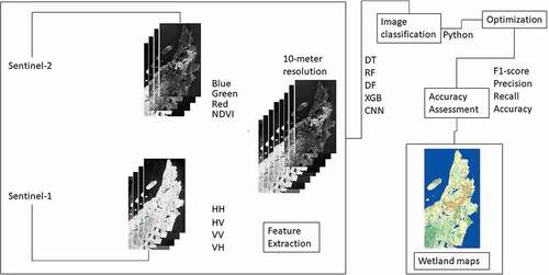
Figure 1 presents the flowchart of the developed methodology in this research. As illustrated, the Methodology can be summarized in four major steps: (1) preparing data and extracting features from Sentinel-1 and −2 imagery, (2) applying tree-based classifiers, including DT, CRF, and DF algorithms, (3) optimizing the parameters of tree-based algorithms in the python programming language, and (4) classifying wetlands and measuring the accuracy indices. These steps are discussed in more details in the following sections.

Figure 1. The flowchart of the methodology used in this research which includes feature extraction, image classification, optimization, accuracy assessment, and wetland mapping procedures

2.1. Study area and remote sensing data

The study site is the Avalon area located at the very eastern portion of Newfoundland, Canada (Figure 2). The Avalon peninsula is approximately 9220 sq. km² with cold winters (winters are not severe) and cool to warm summers. The St. John’s city with an approximate population of 226000 is located on the Avalon peninsula and is the largest city and the capital of Newfoundland. In the study area, wetland habitat and other natural ecosystems can be found. All wetland classes, featured by CWCS, including bog, fen, marsh, swamp, and shallow water are present in the Avalon pilot site, wherein peatlands (i.e. bog and fen) are the most dominant classes. The ground truth data was collected in the summers of 2015 to 2017 by a group of wetland biologists familiar with the study area. Prior to training data collection, possible wetland regions were identified using Google Earth and RapidEye imagery. As a guide for delineation of wetland polygons, Global Positioning System (GPS) points, notes, and photos were taken during field data collection. Moreover, multi-season, multi-year Google Earth imagery were used to improve the accuracy of wetland polygons delineation.

Figure 2. The location of the study area located in Newfoundland, Canada

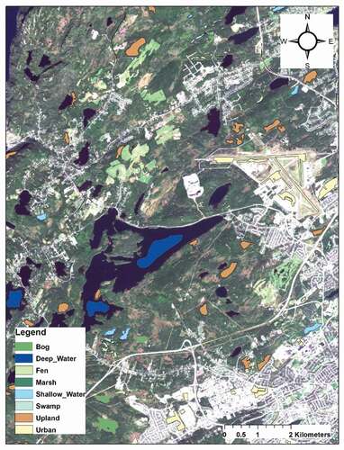
Figure 3 presents several samples of wetland and non-wetland polygons used as the ground truth data.

Figure 3. Examples of ground truth data in the Avalon pilot site (several samples of wetland and non-wetland polygons are used as the ground truth data)

The number of training and testing pixels are presented in Table 1. For reference data preparation, a stratified random sampling technique was used to divide ground truth data into 50% as training and 50% as testing in the Python programming language.

Table 1. Training and testing pixel of wetland samples in the study area of the Avalon, Canada

Class	Number of training pixels	Number of testing pixels
Bog	12,507	12,507
Fen	4012	4012
Marsh	3136	3136
Swamp	2319	2319
Shallow Water	5423	5423
Urban	16,778	16,778
Deep Water	20,557	20,557
Upland	20,852	20,851

In this study, Sentinel-2A level-1 C captured on June 5^th, 2020, is used as the optical imagery. Finding a cloud-free Sentinel-2 imagery was challenging given a nearly permanent cloudy condition within the study area, so the objective was to find images with less than 10% clouds. In addition to the optical imagery bands, several spectral indices, as suggested by previous wetland studies, were used for improving the classification accuracy (Amani et al, 2018; Mahdianpari et al. 2019). For the SAR imagery, a dual-polarized (VV/VH) level-1 Ground Range Detected (GRD) Sentinel-1 image with the ascending orbit captured on June 6^th, 2020, and two dual-polarized (HH/HV) with the descending orbit captured on June 4^th, 2020, were used. We used two dual polarized (HH/HV) images, as the Avalon pilot site was fully covered by the two descending SAR images. In addition to the normalized backscattering coefficients obtained from the SAR imagery, several polarimetric features were also extracted (see Table 2). Notably, the Copernicus Open Access Hub website (https://scihub.copernicus.eu/) was used for SAR and optical data access.

Table 2. Spectral bands, indices, the normalized backscattering coefficients, and polarization features extracted from optical and SAR imagery utilized in this research

Data	Normalized backscattering coefficients/Spectral bands	Polarization features/spectral indices
Sentinel-1	${\sigma }_{VV}^0$, ${\sigma }_{VH}^0$, ${\sigma }_{HH}^0$, ${\sigma }_{HV}^0$	${\sigma }_{HH}^0+{\sigma }_{HV}^0$${\sigma }_{VH}^0+{\sigma }_{VV}^0$$median3by3({\sigma }_{HH}^0$) $median3by3({\sigma }_{HV}^0$) $median3by3({\sigma }_{VH}^0$) $median3by3({\sigma }_{VV}^0$)$median3by3\left({\sigma }_{VH}^0+{\sigma }_{VV}^0\right)$
Sentinel-2	B2, B3, B4, B5, B6, B7, B8, B8A, B11, B12	$EVI=2.4\ast \frac{NIR-R}{\left(NIR+R\right)+1}$$DVI=\left(NIR-R\right)$$RENDVI=\frac{\left(NIR-RE\right)}{\left(NIR+RE\right)}$$NDWI=\frac{\left(NIR-SWIR\right)}{\left(NIR+SWIR\right)}$

2.2. Deep Forest

DF is a non-Neural Network approach proposed by Zhou and Feng (2017) to achieve a performance comparable with deep learning algorithms. As the efficiency and performance of deep learning models greatly depend on the availability of many labeled data, which is problematic for several remote sensing tasks, the main objective for developing DF was to design a non-differentiable deep learning module, capable of dealing with small-scale data (i.e. limited number of training data). It is worth mentioning that due to advances in the deep learning technology, there are a large number of deep learning models that can be efficiently trained from scratch or use transfer learning technique in case there are limited labeled resources. Moreover, there are some Generating Adversarial Network (GAN) models that can create ground truth instances for different applications using a limited number of available ground truths.

One advantage of DF is that its complexity is data-dependent rather than manually designed. Consequently, DF can be used with a low level of model complexity and thus, decreasing the cost of model training, an essential factor for limited amount of training data. Effective characteristics of deep learning methods, includes layer-by-layer processing, sufficient model complexity, and in-model feature transformation. This is in contrast with decision trees, which only employ the original feature representation in their overall learning process without creating any new features (i.e. there is no in-model feature transformation).

The DF can be defined as an ensemble decision tree method that uses a Cascade structure enabling representation learning by several forests where multi-grain scanning can enhance its representational capabilities. In other words, DF is a structural/contextual aware algorithm. It is worth noting that the Cascade structure is developed to employ the effectiveness of layer-by-layer processing in Deep Neural Networks (DNNs). The overall procedure of DF, including multi-grained scanning and Cascade forest, is illustrated in Figure 4 (Zhou and Feng 2017). As illustrated, DF has a similar structure to neural networks albeit with a main difference of rather than building based on neurons layers, whereas DF contains many RFs. Consequently, it can be considered as a multi-layer decision tree ensemble. On the other hand, it has fewer hyper-parameters to be fine-tuned compared to DNNs.

Figure 4. The gcForest overall procedure (gcForest includes multi-grained scanning and Cascade forest layers) (Zhou and Feng 2017)

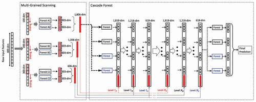
As shown in Figure 5, in each level of Cascade Forest, there are several forests (it can be considered as ensemble of several ensembles) and in each level, for the diversity, there can be different forests. For example, in one level of Cascade Forest, there can be two RF and one XGB classifier. Results obtained by previous levels will be used in the next level, similar to the effective layer-by-layer characteristic of DNN algorithms. It is worth highlighting that as the DF is a contextual or structural aware algorithm, based on the training data, Cascade Forest levels can be automatically determined. As such, it has good performance for tasks with limited number of training data. Finally, results of different forests in the last level of Cascade Forest will be ensembled.

Figure 5. The cascade forest structure (different types of forests such as random forest and extra trees are used in the Cascade Forest)

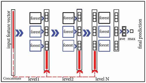
Additionally, the multi-Grained scanning is designed to enhance the Cascade Forest with the use of sliding windows that scan raw features. They are specifically designed for image and sequential data analysis to increase the accuracy of the DF method. It is worth noting that the multi-Grained scanning searches for spatial relationship similar to that of Convolutional Neural Network (CNN) for image data and Recurrent Neural Network (RNN) for sequential data. Notably, although in the original paper the RF method was used as the classifier in the Cascade Forest, we evaluate the performance of the DF algorithm for three different tree-based classifiers of RF (DF-RF), ET (DF-ET), and XGB (DF-XGB).

2.3. Convolutional neural network

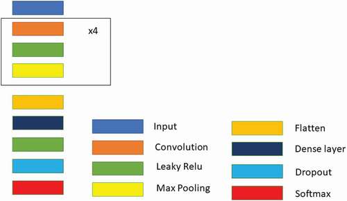
Rather than using an empirical feature design, representation is utilized for the learning process of deep learning algorithms. Deep learning methods are regarded as highly efficient approaches as they automatically learn from internal feature representations (Ji et al. 2018). In remote sensing, CNNs are widely used as they have obtained highly accurate results in complex and high dimensional environments (Mahdianpari et al. 2018; Jamali et al. 2021a). Generally, CNNs have three different layers namely convolutional, pooling, and fully connected. The convolutional layer is the main body of a CNN architecture. It uses several filters that slide through the image. Convolution is regarded as a mathematical operation that merges the input image and filters. To reduce the number of parameters and dimensionality of CNNs, after the convolutional layer, the pooling layer is utilized. It is worth highlighting that the pooling layer reduces the training time and avoids the overfitting issue in CNN methods. Finally, after feature extraction in previous layers, fully connected layer which is like Neural Networks (NNs), is used to classify data into different classes (Jamali et al. 2021a). To compare the results of the tree-based algorithms, specifically the DF method, a CNN method is developed as well in Python (Figure 6 and Table 3). It is worth highlighting that for the convolutional layer, linear activation function is used where padding is set to same.

Table 3. The structure of the developed CNN in this study

Layer Type	Kernel size/ Number of kernels
Convolutional Layer	(2, 2, 64)
Leaky Relu	Alpha = 0.1
Max Pooling	(2, 2)
Convolutional Layer	(3, 3, 128)
Leaky Relu	Alpha = 0.1
Max Pooling	(2,2)
Convolutional Layer	(3, 3, 256)
Leaky Relu	Alpha = 0.1
Max Pooling	(2, 2)
Convolutional Layer	(3, 3, 512)
Leaky Relu	Alpha = 0.1
Max Pooling	(2, 2)
Flatten	~
Dense layer (Linear)	20
Leaky Relu	Alpha = 0.1
Drop out	0.3
Dense layer (Softmax)	8

Figure 6. The developed CNN architecture in this study

2.4. Pre-processing of satellite imagery

The optical image of Sentinel-2 is atmospherically and radiometrically corrected using sen2cor tool (Louis et al. 2016) in the SNAP software. Geocoded backscatter intensity images were extracted from three Sentinel-1 images using SNAP. As such, orbital metadata was updated, and then Sentinel-1 imagery were radiometrically calibrated. This was followed by the conversion of unitless backscattering intensity images into normalized backscatter coefficients ${\sigma }^0$ in dB values, which is the standard unit for the representation of SAR backscattering. Next, a Lee Sigma filter with a window size of 7 by 7 was applied to reduce the inherent speckle noises within SAR imagery. Finally, the imagery was geometrically corrected with the Range-Doppler terrain correction method.

2.5. Accuracy assessment

The classification results are evaluated in terms of several accuracy indices, including mean overall accuracy, precision, recall, and F1-score statistical indices (Equations 1(1) $Auracy=\frac{\left(Truepositive+Truenegative\right)}{Totalnumberofpixels}$(1) –4(4) $F1-score=2\ast \frac{\mathrm{P}\mathrm{r}\mathrm{e}\mathrm{c}\mathrm{i}\mathrm{s}\mathrm{i}\mathrm{o}\mathrm{n}\ast \mathrm{R}\mathrm{e}\mathrm{c}\mathrm{a}\mathrm{l}\mathrm{l}}{\mathrm{P}\mathrm{r}\mathrm{e}\mathrm{c}\mathrm{i}\mathrm{s}\mathrm{i}\mathrm{o}\mathrm{n}+\mathrm{R}\mathrm{e}\mathrm{c}\mathrm{a}\mathrm{l}\mathrm{l}}$(4) ).

(1) $Auracy=\frac{\left(Truepositive+Truenegative\right)}{Totalnumberofpixels}$(1)

(2) $Precision=\frac{\mathrm{T}\mathrm{r}\mathrm{u}\mathrm{e}\mathrm{p}\mathrm{o}\mathrm{s}\mathrm{i}\mathrm{t}\mathrm{i}\mathrm{v}\mathrm{e}}{\left(Truepositive+Falsepositive\right)}$(2)

(3) $Recall=\frac{\mathrm{T}\mathrm{r}\mathrm{u}\mathrm{e}\mathrm{p}\mathrm{o}\mathrm{s}\mathrm{i}\mathrm{t}\mathrm{i}\mathrm{v}\mathrm{e}}{\left(Truepositive+Falsenegative\right)}$(3)

(4) $F1-score=2\ast \frac{\mathrm{P}\mathrm{r}\mathrm{e}\mathrm{c}\mathrm{i}\mathrm{s}\mathrm{i}\mathrm{o}\mathrm{n}\ast \mathrm{R}\mathrm{e}\mathrm{c}\mathrm{a}\mathrm{l}\mathrm{l}}{\mathrm{P}\mathrm{r}\mathrm{e}\mathrm{c}\mathrm{i}\mathrm{s}\mathrm{i}\mathrm{o}\mathrm{n}+\mathrm{R}\mathrm{e}\mathrm{c}\mathrm{a}\mathrm{l}\mathrm{l}}$(4)

3. Results

3.1. Hyper-parameter tuning

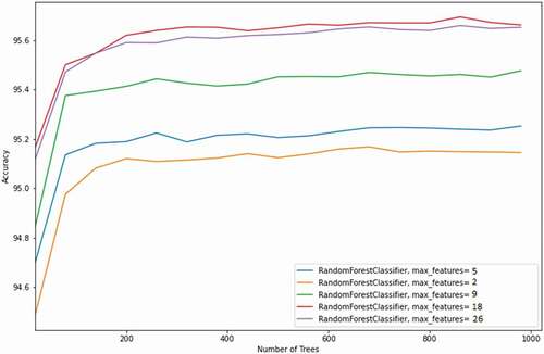
For the CRF algorithm, different values for the nTree were used and five different values, including 2, 5, 9, 18, and 28, were considered as the maximum number of features. Notably, the optimal classifier was obtained by setting the maximum number of features as 18. It is worth mentioning that generalization error can be influenced by the number of randomly selected features (i.e. the maximum number of features). The strength of individual trees will improve by increasing the maximum number of features, although it increases the correlation between trees which may reduce the generalization strength of a forest. The value of the maximum number of features as discussed in the previous sections highly depends on the complexity of the input data. As a result, the value of the maximum number of features should be measured as a tuning parameter for different issues (Friedman, Trevor, and Robert 2001). Setting the maximum number of features to 28 achieved better results than that of 9, 5, and 2. As illustrated in Figure 7, accuracy substantially improved by increasing nTree from 20 to 200, after which the classification accuracy is relatively stable. As indicated in Figure 7, the optimal classification model with an accuracy value of 95.66% was obtained with the nTree of 860, although it only improved the classification accuracy by 0.07% compared to the CRF model with nTree of 200.

Figure 7. Classification accuracy of the CRF classifier for different values of the number of trees and the maximum number of features

For optimizing the results of the DF and CXGB classifiers, different values for the nTree and the maximum of depth were considered. The classification results obtained by four classifiers, namely RF (DF-RF), XGB (DF-XGB), Extra Trees (DF-ET), and CXGB, implemented in the python programming language were evaluated (Figure 8 and Figure 9). First, the maximum depth was set to 5, and the classification accuracy of the DF and CXGB were evaluated based on different nTree. As illustrated in Figure 8, the highest classification accuracy was obtained by the DF-XGB classifier with an accuracy of 97.63%, followed by the CXGB with an accuracy of 96.71% with the nTree of 500. Increasing the nTree substantially improved the classification accuracy obtained by the DF-XGB and CXGB. The XGB classifier requires a high number of trees for reaching its full potential. Notably, to improve the classification accuracy of an XGB classifier with a low maximum of depth (e.g. less than 5), the nTree should be substantially increased. Results indicated that the accuracy of the DF-RF and DF-ET classifiers were approximately stable by increasing the nTree from 100 to 500. The reason for better classification accuracy of DF-XGB and CXGB by increasing the nTree should be due to their ensemble methodology. The CRF and ET classifiers are bagging methods in which each tree is constructed independently and at the end of the training process, trees are ensembled, while the XGB classifier is a boosting method building one tree at a time. The XGB algorithm has a forward stage-wise manner which uses a weak learner to overcome the shortcomings of the previous weak learners (i.e. existing trees). In other words, the XGB algorithm starts the tree ensemble from the beginning of the classification process, while the CRF and ET methods do the tree ensemble at the end of the training process. As a result, the DF-XGB and CXGB classifiers produce better classification accuracy over the DF-RF and DF-ET while increasing the nTree.

Figure 8. Classification accuracies obtained by the Deep Forest for different values of the number of trees for DF-RF, DF-XGB, and DF-ET (the maximum of depth was set to 5)

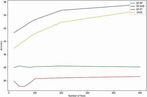
Figure 9. Classification accuracies obtained by the Deep Forest for different values of the maximum depth for classifiers of DF-RF, DF-XGB, and DF-ET classifiers (the number of trees was set to 200)

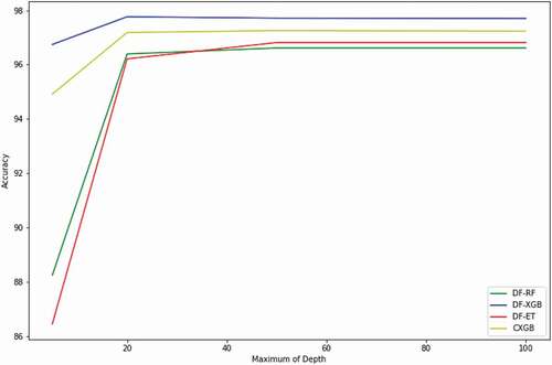
We evaluated the classification accuracies of the DF and CXGB algorithms for different maximum of depth. In all four cases, accuracies improved by increasing substantially the maximum of depth from 5 to 20, after which minimal changes in accuracies were observed (Figure 9). In particular, by increasing the maximum of depth, results showed that the highest accuracy of 97.71% was achieved by the DF-XGB, followed by the CXGB (with an accuracy of 97.25%) classifiers with a maximum of depth of 50. Additionally, the DF-ET method was superior compared to DF-RF when the maximum of depth varied between 50 and 100. Notably, results of DF-RF and DF-ET classifiers were considerably improved by increasing the maximum of depth from 5 to 20. The DF-XGB and CXGB classifiers had consistent results while increasing the maximum of depth. The reason can be explained by different ensemble methods of the DF-ET and DF-RF classifiers (i.e. Bagging method) over the DF-XGB and CXGB classifiers (i.e. Boosting method) as mentioned before. With an equal nTree, a higher complexity (i.e. a higher number of the maximum of depth) has more influence on the Bagging methods of DF-RF and DF-ET compared to the Boosting methods of DF-XGB and CXGB.

3.2. Classification maps

In this section, results of the optimized DT, CRF, CXGB, the developed CNN, and DF are evaluated and discussed in terms of statistical indices, including F1-score, precision, and recall. The presented results in Table 3 were achieved by the optimized tree-based classifiers and the CNN classifier. The results demonstrated a high level of agreement between the ground truth and predicated non-wetland classes of urban, deep water, and upland areas for the three classifiers. This is attributed to the availability of the more training samples for these classes compared to wetland classes. Creating training samples for non-wetland classes due to their less possible spectral similarity, is much easier. Generally, even non-expert users can differentiate and recognize these non-wetland classes in the optical imagery. However, wetland classes are hardly distinguishable even in the field due to their similar visual appearances and in the satellite imagery due to their similar spectral signatures. This necessitates knowledge-expertise for delineating wetland training data, which could be labor-intensive and costly.

As shown in Table 4, the DF classifier outperforms the other tree-based classifiers of the DT, CRF, and CXGB, as well as the developed CNN classifier with F1-score of 0.97, 0.96, 0.90, 0.90, 0.87 for bog, shallow water, fen, marsh, and swamp wetland classes, respectively. In addition, the CXGB classifier is superior to the other algorithms with F1-score of 0.97, 0.96 0.88, 0.87, and 0.83 for the recognition of bog, shallow water, marsh, fen, and swamp, respectively. The developed CNN has better performance against the CRF method for the classification of marsh and shallow water with F1-score of 0.88 and 0.96, respectively. However, the CRF classifier is superior to the developed CNN algorithm for the classification of fen and swamp wetland classes with F-1 score of 0.76 and 0.74, respectively. The CRF classifier had better performance over the DT algorithm with F1-score of 0.95, 0.94, 0.83, 0.76, and 0.74, for discriminating shallow water, bog, marsh, fen, and swamp classes, respectively. Finally, the DT classifier with F1-scores of 0.92, 0.90, 0.71, 0.62, and 0.60 had the least performance for classifying wetland classes of shallow water, bog, marsh, fen, and swamp, respectively (Table 4).

Table 4. Results evaluation of the developed algorithms for the classification of wetlands in terms of F1-score, precision, and recall statistical indices

	Bog	Fen	Marsh	Swamp	Shallow water	Urban	Deep Water	Upland	Accuracy
DT									92.50
F1-score	0.90	0.62	0.71	0.60	0.92	0.98	0.99	0.95
Precision	0.90	0.63	0.71	0.60	0.93	0.98	0.99	0.95
Recall	0.90	0.62	0.71	0.60	0.92	0.99	0.99	0.95
CRF									95.66
F1-score	0.94	0.76	0.83	0.74	0.95	0.99	0.99	0.97
Precision	0.96	0.70	0.78	0.68	0.97	0.99	0.99	0.98
Recall	0.93	0.83	0.88	0.81	0.93	0.99	0.99	0.96
CXGB									97.25
F1-score	0.97	0.87	0.88	0.83	0.96	1	1	0.98
Precision	0.97	0.84	0.85	0.77	0.97	1	1	0.99
Recall	0.96	0.9	0.91	0.89	0.95	0.99	1	0.97
CNN									96.03
F1-score	0.94	0.7	0.88	0.71	0.96	1	1	0.97
Precision	0.95	0.62	0.89	0.62	0.97	1	0.99	1
Recall	0.92	0.81	0.86	0.81	0.95	1	1	0.95
DF-XGB									97.76
F1-score	0.97	0.90	0.90	0.87	0.96	0.99	0.99	0.99
Precision	0.97	0.90	0.88	0.85	0.97	0.99	0.99	0.99
Recall	0.98	0.91	0.91	0.89	0.96	0.99	0.99	0.98

As shown in Table 5, all tree-based classifiers were successful for distinguishing the non-wetland classes. For the DT classifier, there were several misclassifications between the swamp and upland classes. This could be due to their similar spectral reflectance between these two wetland classes given their dominant tree-based structure. As indicated in Table 5, confusion occurred between bog, fen, and marsh classes, particularly between the first two classes. The reason is due to their similar spectral reflectance. These wetland classes may have similar vegetation patterns, such as wet soils, saturated vegetation, and some emergent vegetation, making classification of these classes challenging. Overall, the classification results revealed more advanced classification technique can improve accuracies of wetland classification. For example, an ensemble of tree classifiers in the CXGB and CRF models outperformed the single DT classifier, whereas an ensemble of forests in DF attained the higher accuracy compared to the CRF. For instance, precision values achieved by the DT classifier for marsh, fen, and swamp classes was equal to 0.72, 0.62, and 0.60, respectively. Based on the F-1 score, classification accuracies were noticeably improved for the classes of marsh, fen, and swamp by increasing the number of trees in the CRF classifier reaching 0.83, 0.76, and 0.74, respectively. The DF classifier significantly improved the classification accuracies of fen, marsh, and swamp classes with F-1 score values of 0.90, 0.90, and 0.87, respectively (Table 5). Notably, the higher classification accuracy of the bog class compared to the other wetland classes is possibly due to the higher number of training samples for bog compared to other wetland classes.

Table 5. The confusion matrix of the developed algorithms for the classification of wetlands

DT	Bog	Fen	Marsh	Swamp	Shallow water	Urban	Deep water	Upland
Bog	11,227	824	149	150	14	38	0	105
Fen	804	2522	162	198	3	49	0	274
Marsh	172	160	2239	102	335	31	2	95
Swamp	153	205	124	1402	1	7	0	427
Shallow water	15	4	281	3	5037	1	82	0
Urban	59	50	52	10	1	16,492	0	114
Deep Water	0	0	1	0	98	0	20,458	0
Upland	76	309	124	460	1	91	0	19,791
CRF	Bog	Fen	Marsh	Swamp	Shallow water	Urban	Deep water	Upland
Bog	12,055	218	57	93	18	9	0	57
Fen	753	2816	50	119	0	11	0	263
Marsh	83	129	2437	44	314	47	1	81
Swamp	76	113	69	1584	0	0	0	477
Shallow water	10	0	98	0	5240	1	74	0
Urban	25	13	16	2	0	16,715	0	7
Deep Water	0	0	0	0	36	0	20,521	0
Upland	26	92	28	107	0	103	0	20,496
CXGB	Bog	Fen	Marsh	Swamp	Shallow water	Urban	Deep water	Upland
Bog	12,193	154	39	52	14	5	0	50
Fen	380	3386	42	66	0	9	0	129
Marsh	60	70	2653	42	235	27	1	48
Swamp	58	73	50	1791	0	0	0	347
Shallow water	7	0	93	0	5258	1	64	0
Urban	5	7	13	3	0	16,745	0	5
Deep Water	0	0	0	0	21	0	20,536	0
Upland	17	53	23	51	0	43	0	20,665
CNN	Bog	Fen	Marsh	Swamp	Shallow water	Urban	Deep water	Upland
Bog	11,918	452	40	80	5	0	0	12
Fen	876	2475	119	162	1	1	0	378
Marsh	27	49	2785	42	170	10	1	52
Swamp	135	84	91	1447	1	0	0	561
Shallow water	5	0	174	0	5238	0	6	0
Urban	0	2	6	1	0	16,720	0	43
Deep Water	0	0	0	0	115	0	20,442	0
Upland	0	4	9	46	0	34	0	20,759
DF-XGB	Bog	Fen	Marsh	Swamp	Shallow water	Urban	Deep water	Upland
Bog	12,148	212	38	56	11	4	0	38
Fen	207	3613	34	70	0	7	0	81
Marsh	36	52	2761	41	195	15	0	36
Swamp	41	62	35	1967	0	0	0	214
Shallow water	7	0	120	0	5250	1	45	0
Urban	1	2	13	3	0	16,735	0	24
Deep Water	0	0	0	0	31	0	20,526	0
Upland	9	47	23	83	0	21	0	20,669

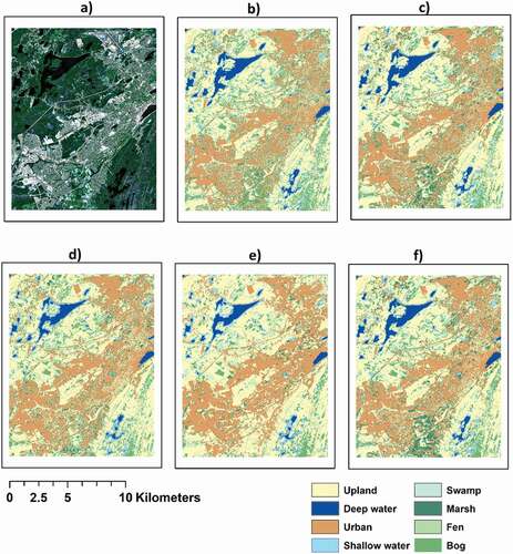
Wetland maps obtained from the best performed tree-based classifiers are illustrated in Figure 10.

Figure 10. Wetland classification maps of the Avalon pilot study using a) study area in true color b) Decision Tree, c) Conventional Random Forest, d) Conventional Extreme Gradient Boosting, e) the developed Convolutional Neural Network, and f) Deep Forest (DF-XGB)

4. Discussion

In this section, the classification accuracies of the CRF classifier obtained from different datasets are evaluated and discussed. Results obtained from the Sentinel-1 imagery showed that there is a high level of agreement between ground truth data and the predicted classes for non-wetland classes of deep water and upland. Based on the F-1 score, the CRF classifier based on SAR data poorly classified fen, marsh, and swamp classes. Classification results obtained from single source optical data were much better compared to single source SAR data, specifically for discriminating the wetland classes of bog, fen, marsh, swamp, and shallow water. However, the synergic use of Sentinel-1 and Sentinel-2 produced the highest results in terms of accuracy, F1-score, precision, and recall statistical indices (Table 6). The results are in line with the previous research studies regarding the superiority of Sentinel 2 over Sentinel 1 and superiority of a synergic use of Sentinel 1 and Sentinel 2 over a single source of SAR or optical imagery for the wetland classification.

Table 6. Classification results of the CRF algorithm obtained from single source SAR (S1), optical (S2), and multi-source (S1 and S2) data

Data sets	Bog	Fen	Marsh	Swamp	Shallow water	Urban	Deep water	Upland	Accuracy
S1									79.33
F1-score	0.72	0.3	0.38	0.21	0.66	0.78	0.94	0.87
Precision	0.79	0.22	0.27	0.13	0.6	0.75	0.99	0.94
Recall	0.66	0.45	0.62	0.52	0.73	0.82	0.9	0.8
S2									94.14
F1-score	0.92	0.63	0.79	0.62	0.94	0.99	0.99	0.96
Precision	0.96	0.55	0.74	0.54	0.94	0.99	0.99	0.98
Recall	0.89	0.74	0.84	0.72	0.94	0.99	0.99	0.94
S1 and S2									95.66
F1-score	0.94	0.76	0.83	0.74	0.95	0.99	0.99	0.97
Precision	0.96	0.7	0.78	0.68	0.97	0.99	0.99	0.98
Recall	0.93	0.83	0.88	0.81	0.93	0.99	0.99	0.96

The inclusion of SAR data improved the accuracy of fen, swamp, marsh, and bog by 13%, 12%, 4%, and 2% compared to single source optical data based on the F1-score (see S2 vs S1 and S2 in Table 6). Regarding SAR features, ${\sigma }_{HV}^0$ observations are useful for the classification of wetlands as these cross-polarized observations are generated by the volume scattering within vegetation canopies. Consequently, ${\sigma }_{HV}^0$ observations are sensitive to vegetation structure. The ${\sigma }_{VV}^0$ observations are sensitive to soil moisture and are useful for discriminating wetland vegetation classes at their early stages, given the dominant surface scattering mechanisms at this time. Another ideal SAR observation for the identification of wetlands is ${\sigma }_{HH}^0$, which is sensitive to double-bounce scattering for flooded vegetation. Furthermore, ${\sigma }_{HH}^0$ is less sensitive to water surface roughness compared to ${\sigma }_{VV}^0$, which can be used for the recognition of water bodies from non-water classes (Mahdianpari et al. 2019, 2017).

To investigate the optimal number of Cascade Forest levels for wetland mapping, we evaluated the performance of the DF-ET classifier for different maximum number of Cascade Forest levels. As evident in Table 7, the highest level of accuracy was achieved by setting the maximum cascade level to two with an accuracy of 95.51%, after which the classification accuracy is stable. It can be explained that the optimal DF-ET model was reached by two Cascade levels, after which increasing the number of the Cascade Forest levels had no effect on the classification results. It is worth highlighting that the optimal Cascade Forest Level depends on the available training data.

Table 7. Accuracy of Deep Forest with classifier of Extra Trees for different Cascade levels (in percent)

Maximum Cascade levels	Accuracy
1	94.81
2	95.51
3	95.51
4	95.51
5	95.51
10	95.51

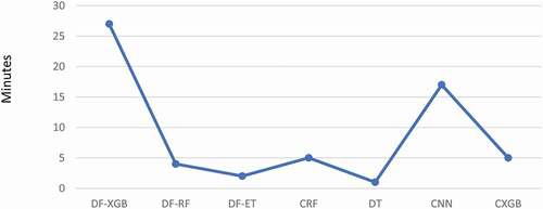
An important factor for the selection of the best-suited algorithm for wetland classification is the cost of a specific classifier in terms of processing time. As illustrated by Figure 11, although the DF-XGB had the best performance relative to other tree-based methods, it required the longest training time of 27 minutes. DT, on the other hand, required the least training time of less than a minute, given its less complexity compared to other examined methods in this study. The developed CNN, the optimized CXGB, the optimized CRF, and DF-RF required training time of 17, 5, 5, 4 minutes, respectively. The DF-ET required about 2 minutes for its training and achieved a greater wetland classification accuracy compared to both DF-RF and CRF.

Figure 11. Training time of the tree-based classifiers of Deep Forest (DF-ET, DF-RF, and DF-XGB), Conventional Random Forest, Conventional Extreme Gradient Boosting, and the developed Convolutional Neural Network

For the cost complexity, considering $n$ number of training samples, $m_{try}$ number of features, and $n_{tree}$ number of trees, the training time complexity of building a tree is approximately equal to $O\left(m_{try}\times n\times logn\right)$. As such, the computation cost of building a Forest with $n_{tree}$ trees would be about $O\left(n_{tree}\times m_{try}\times n\times logn\right)$. For the DF classifier as there are several Cascade levels and each Cascade layer has several forests, time complexity will be multiplied by the number of levels and the number of forests in each Cascade level.

Based on the results and considering the complexity and dynamic nature of wetlands in the study area of the Avalon, the DF algorithm had a high capability of correctly differentiating between different wetland classes (with F-1 scores higher than 0.87 for all wetland classes). Results of the trained algorithms in the study area of the Avalon were used for the prediction of the wetland and non-wetland classes in a more complex region of the Grand Falls with different spatial and temporal characteristics where the DF-XGB classifier had better performance in terms of accuracy (Appendix A).

5. Conclusion

In this study, we used the DF classifier which is a non-neural deep learning method and evaluated its performance against three other well-known tree-based algorithms of the DT, CRF, and CXGB for the classification of high-resolution complex wetland mapping in the pilot site of Avalon. Results showed that the DF algorithm had better performance over the optimized CXGB by 14%, 13%, 7%, 3%, and 1% for the classification of fen, swamp, marsh, bog, and shallow water wetland classes, respectively. In addition, the results of CXGB were improved by 4%, 3%, and 2% for the classification of swamp, fen, and marsh by the DF-XGB, respectively.

The CRF, CXGB and DF methods obtained better classification accuracy to a certain level of complexity. We trained the DF classifier with the use of tree different algorithms of XGB, Extra Trees, and RF where the DF-XGB classifier was superior to the other two methods in terms of classification accuracy, however the DF-ET was superior in terms of training time. The DF-XGB and CXGB classifiers had significant superiority with a low level of complexity over the DF-RF and DF-ET classifiers where the maximum depth was set to 5 and the nTree was set to 20. Increasing the level of complexity of DF specifically, increasing the maximum of depth significantly improved the results of both DF-RF and DF-ET classifiers where they obtained a level of classification accuracy comparable with the DF-XGB and CXGB methods. Moreover, with a lower number of depths, the DF-RF classifier was superior to the DF-ET method. Increasing the number of depths significantly improved the results achieved by the DF-ET classifier outperforming the DF-RF method (Figures 7 and Figures 8). Additionally, in this study we utilized a synergic use of SAR and optical imagery of Sentinel 1 and Sentinel 2 imagery where results confirmed that extracted SAR backscattering coefficients and polarization features could substantially improve the results of wetland classification. In terms of the F1-score statistical index, results of wetland classes of fen, swamp, marsh, and bog obtained by the optical image of Sentinel 2 was improved by 13%, 12%, 4%, and 2% with the inclusion of SAR extracted features (Table 5). Although the DF-XGB method was superior to the other classifiers, its higher level of time cost would be a burden for applications with limited processing resources. As a result, in the future, to achieve better classification results for wetland mapping, we will focus on the ensemble of DF-ET classifier (that has a lower training time) with well-known CNNs with low hyperparameters.

Code, data, and materials availability

The codes generated and analyzed during the current study are available in GitHub (https://github.com/aj1365/DeepForest-Wetland-Paper).

Disclosure statement

No potential conflict of interest was reported by the author(s).

Appendix A.

To demonstrate the spatiotemporal transferability of the proposed algorithm, we evaluated the capability of pre-trained ML methods on a different pilot site located in Grand Fall, NL, with a complex wetland structure and relatively different climatic and biologic characteristics (see Figure A1 and Table A1).

Figure A1. Wetland classification maps of the Grand Falls area using a) study area in true color b) Decision Tree, c) Conventional Random Forest, d) Conventional Extreme Gradient Boosting, e) the developed Convolutional Neural Network, and f) Deep Forest (DF-XGB)

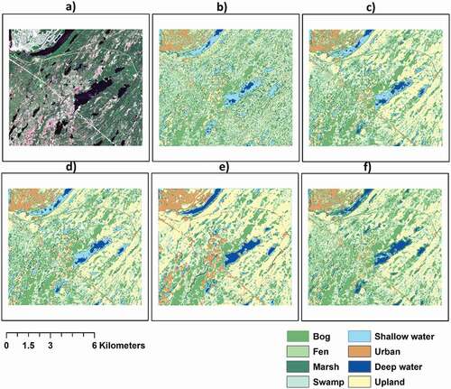
Table A1. The confusion matrix of the pre-trained algorithms (trained on the Avalon dataset) for the classification of wetlands evaluated in Grand Falls

DT	Bog	Fen	Marsh	Swamp	Shallow water	Urban	Deep water	Upland
Bog	20,550	3140	1089	380	116	495	0	774
Fen	9634	3223	1158	424	53	1306	0	1248
Marsh	739	828	2309	325	1807	982	486	751
Swamp	388	1012	639	991	2	11	0	1157
Shallow water	95	32	686	14	1485	5	217	6
Urban	737	874	634	117	5	8984	0	606
Deep Water	0	0	28	0	712	0	7377	0
Upland	82	1283	2497	996	0	7	0	11,052
CRF	Bog	Fen	Marsh	Swamp	Shallow water	Urban	Deep water	Upland
Bog	23,885	1307	642	145	33	235	0	297
Fen	11,914	2580	815	315	0	737	0	685
Marsh	846	683	3390	185	1043	1026	552	502
Swamp	329	578	405	1114	0	2	0	1772
Shallow water	84	8	1013	8	1163	3	257	4
Urban	643	473	448	54	0	10,180	0	159
Deep Water	0	0	13	0	625	0	7479	0
Upland	6	169	36	176	0	11	0	15,519
CXGB	Bog	Fen	Marsh	Swamp	Shallow water	Urban	Deep water	Upland
Bog	24,064	784	736	169	56	282	0	453
Fen	11,732	1821	1016	316	8	763	0	1390
Marsh	725	511	3160	217	1403	931	703	577
Swamp	297	682	428	1071	0	2	0	1720
Shallow water	58	8	421	15	1546	4	485	3
Urban	322	302	314	29	2	10,748	0	240
Deep Water	0	0	49	0	344	0	7724	0
Upland	2	376	43	264	0	4	0	15,228
CNN	Bog	Fen	Marsh	Swamp	Shallow water	Urban	Deep water	Upland
Bog	23,704	934	331	607	83	203	0	682
Fen	9607	4922	570	796	38	143	0	970
Marsh	380	515	3786	298	745	1115	1033	405
Swamp	193	37	554	792	0	65	0	2559
Shallow water	49	0	766	12	940	23	742	8
Urban	37	167	409	67	1	10,501	0	780
Deep Water	8601	0	0	0	0	0	8117	0
Upland	137	4	30	3	0	9	0	15,735
DF-XGB	Bog	Fen	Marsh	Swamp	Shallow water	Urban	Deep water	Upland
Bog	24,401	1041	527	78	32	130	0	335
Fen	12,472	2459	611	198	2	316	0	988
Marsh	740	901	3731	172	456	996	790	441
Swamp	362	779	361	1042	0	1	0	1655
Shallow water	85	15	1032	9	836	3	556	4
Urban	846	500	361	32	0	10,055	0	163
Deep Water	0	0	444	0	64	0	7609	0
Upland	2	279	22	231	0	4	0	15,379

References

- Altwaijry, N., and I. Al-Turaiki. 2021. “Arabic Handwriting Recognition System Using Convolutional Neural Network.” Neural Computing & Applications 33 (7): 2249–2261. doi:https://doi.org/10.1007/s00521-020-05070-8.
- Amani, M., B. Salehi, S. Mahdavi, and B. Brisco. 2018. “Spectral Analysis of Wetlands Using Multi-Source Optical Satellite Imagery.” ISPRS Journal of Photogrammetry and Remote Sensing 144: 119–136. doi:https://doi.org/10.1016/j.isprsjprs.2018.07.005.
- Berhane, T. M., C. R. Lane, Q. Wu, B. C. Autrey, O. A. Anenkhonov, V. V. Chepinoga, and H. Liu. 2018. “Decision-Tree, Rule-Based, and Random Forest Classification of High-Resolution Multispectral Imagery for Wetland Mapping and Inventory.” Remote Sensing 10 (4): 580. doi:https://doi.org/10.3390/rs10040580.
- Board, M. A. 2005. Millennium Ecosystem Assessment. Washington, DC: New Island.
- Davis, P., F. Aziz, M. T. Newaz, W. Sher, and L. Simon. 2021. “The Classification of Construction Waste Material Using a Deep Convolutional Neural Network.” Automation in Construction 122 (February): 103481. doi:https://doi.org/10.1016/j.autcon.2020.103481.
- Friedman, J., H. Trevor, and T. Robert. 2001. The Elements of Statistical Learning. Vol. 1. 10 vols. New York: Springer series in statistics.
- Gardner R. C., and N. C. Davidson. 2011. “The Ramsar Convention.” In: LePage B. (eds),Wetlands. Dordrecht: Springer. doi:https://doi.org/10.1007/978-94-007-0551-7_11.
- Jamali, A. 2020a. “Land Use Land Cover Mapping Using Advanced Machine Learning Classifiers: A Case Study of Shiraz City, Iran.” Earth Science Informatics 13 (4): 1015–1030. doi:https://doi.org/10.1007/s12145-020-00475-4.
- Jamali, A. 2020b, July. “Improving Land Use Land Cover Mapping of a Neural Network with Three Optimizers of Multi-Verse Optimizer, Genetic Algorithm, and Derivative-Free Function.” The Egyptian Journal of Remote Sensing and Space Science. doi:https://doi.org/10.1016/j.ejrs.2020.07.001.
- Jamali, A., M. Mahdianpari, B. Brisco, J. Granger, F. Mohammadimanesh, and B. Salehi. 2021a. “Comparing Solo versus Ensemble Convolutional Neural Networks for Wetland Classification Using Multi-Spectral Satellite Imagery.” Remote Sensing 13 (11): 2046. doi:https://doi.org/10.3390/rs13112046.
- Jamali, A., M. Mahdianpari, B. Brisco, J. Granger, F. Mohammadimanesh, and B. Salehi. 2021b. “Wetland Mapping Using Multi-Spectral Satellite Imagery and Deep Convolutional Neural Networks: A Case Study in Newfoundland and Labrador, Canada.” Canadian Journal of Remote Sensing. April. Taylor & Francis. 1–18. doi:https://doi.org/10.1080/07038992.2021.1901562.
- Ji, S., C. Zhang, A. Xu, Y. Shi, and Y. Duan. 2018. “3D Convolutional Neural Networks for Crop Classification with Multi-Temporal Remote Sensing Images.” Remote Sensing 10 (2): 75. doi:https://doi.org/10.3390/rs10010075.
- Liu, K., S. Wu, Z. Luo, Z. Gongze, X. Ma, Z. Cao, and H. Li. 2021 February. “An Intelligent Fault Diagnosis Method for Transformer Based on IPSO-GcForest.” In Mathematical Problems in Engineering 2021, edited by M. Kunicki. Hindawi: 6610338. doi:https://doi.org/10.1155/2021/6610338.
- Louis, J., V. Debaecker, B. Pflug, M. Main-Knorn, J. Bieniarz, U. Mueller-Wilm, E. Cadau, and F. Gascon. 2016. Sentinel-2 Sen2Cor: L2A Processor for Users, 1–8. Spacebooks Online.
- Mahdianpari, M., B. Salehi, F. Mohammadimanesh, and M. Motagh. 2017. “Random Forest Wetland Classification Using ALOS-2 L-Band, RADARSAT-2 C-Band, and TerraSAR-X Imagery.” ISPRS Journal of Photogrammetry and Remote Sensing 130: 13–31. doi:https://doi.org/10.1016/j.isprsjprs.2017.05.010.
- Mahdianpari, M., B. Salehi, F. Mohammadimanesh, S. Homayouni, and E. Gill. 2019. “The First Wetland Inventory Map of Newfoundland at a Spatial Resolution of 10 M Using Sentinel-1 and Sentinel-2 Data on the Google Earth Engine Cloud Computing Platform.” Remote Sensing 11 (1): 43. doi:https://doi.org/10.3390/rs11010043.
- Mahdianpari, M., B. Salehi, M. Rezaee, F. Mohammadimanesh, and Y. Zhang. 2018. “Very Deep Convolutional Neural Networks for Complex Land Cover Mapping Using Multispectral Remote Sensing Imagery.” Remote Sensing 10 (7): 1119. doi:https://doi.org/10.3390/rs10071119.
- Maxwell, A. E., T. A. Warner, and F. Fang. 2018. “Implementation of Machine-Learning Classification in Remote Sensing: An Applied Review.” International Journal of Remote Sensing 39 (9): 2784–2817. doi:https://doi.org/10.1080/01431161.2018.1433343.
- Oduro Appiah, J., C. Opio, O. Venter, S. Donnelly, and D. Sattler. 2021 (March). “Assessing Forest Cover Change and Fragmentation in Northeastern British Columbia Using Landsat Images and a Geospatial Approach.” Earth Systems and Environment 5 (2): 253–270. doi:https://doi.org/10.1007/s41748-021-00207-8.
- Rubec, C. 2018. “The Canadian Wetland Classification System.” In Finlayson C.M. et al. (eds). The Wetland Book, 1577–1581. Dordrecht, The Netherlands: Springer. doi:https://doi.org/10.1007/978-90-481-9659-3_340
- Slagter, B., N. E. Tsendbazar, A. Vollrath, and J. Reiche. 2019. “Mapping Wetland Characteristics Using Temporally Dense Sentinel-1 and Sentinel-2 Data: A Case Study in the St. Lucia Wetlands, South Africa.” International Journal of Applied Earth Observation and Geoinformation 86: 102009. doi:https://doi.org/10.1016/j.jag.2019.102009.
- Song, H., X.-Y. Han, C. E. Montenegro-Marin, and S. Krishnamoorthy. 2021. “Secure Prediction and Assessment of Sports Injuries Using Deep Learning Based Convolutional Neural Network.” Journal of Ambient Intelligence and Humanized Computing 12 (3): 3399–3410. doi:https://doi.org/10.1007/s12652-020-02560-4.
- Sun, X., P. Wang, C. Wang, Y. Liu, and K. Fu. 2021. “PBNet: Part-Based Convolutional Neural Network for Complex Composite Object Detection in Remote Sensing Imagery.” ISPRS Journal of Photogrammetry and Remote Sensing 173 (March): 50–65. doi:https://doi.org/10.1016/j.isprsjprs.2020.12.015.
- Tiner, R. W. 2015. “Wetlands: An Overview.” In Remote Sensing of Wetlands: Applications and Advances, edited by R. W. Tiner, M. W. Lang, and V. V. Klemas, 20–35. Boca Raton, FL: CRC Press.
- Wenping, M., Y. Hui, Y. Wu, X. Yunta, H. Tao, J. Licheng, and H. Biao. 2019. “Change Detection Based on Multi-Grained Cascade Forest and Multi-Scale Fusion for SAR Images.” Remote Sensing 11 (2): 142. doi:https://doi.org/10.3390/rs11020142
- Yu, B., C. Chen, X. Wang, Z. Yu, A. Ma, and B. Liu. 2021. “Prediction of Protein–Protein Interactions Based on Elastic Net and Deep Forest.” Expert Systems with Applications 176 (August): 114876. doi:https://doi.org/10.1016/j.eswa.2021.114876.
- Zhang, J., H. Hongjun, and B. Zhou. 2020. “SAR Target Classification Based on Deep Forest Model.” Remote Sensing 12 (1): 128. doi:https://doi.org/10.3390/rs12010128
- Zhang, J., and H. Song. 2021. “Multi-Feature Fusion for Weak Target Detection on Sea-Surface Based on FAR Controllable Deep Forest Model.” Remote Sensing 13 (4): 812. doi:https://doi.org/10.3390/rs13040812.
- Zhang, Y., K. Fu, H. Sun, X. Sun, X. Zheng, and H. Wang. 2018. “A Multi-Model Ensemble Method Based on Convolutional Neural Networks for Aircraft Detection in Large Remote Sensing Images.” Remote Sensing Letters 9 (1): 11–20. Taylor & Francis. doi:https://doi.org/10.1080/2150704X.2017.1378452.
- Zhiyuan, S., M. Li, J. Zhang, B. Hu, G. Qi, and Y. Zhu. 2021. “Transient Voltage Stability Assessment Method Based on GcForest.” Journal of Physics. Conference Series 1914 (1): IOP Publishing: 012025. doi:https://doi.org/10.1088/1742-6596/1914/1/012025.
- Zhou, Z.-H., and J. Feng. 2017. “Deep Forest.” ArXiv Preprint no. arXiv:1702.08835.