Recent trends in the timing of the growing season in New Zealand’s natural and semi-natural grasslands

ABSTRACT

We investigate the temporal dynamics of shifts in phenological responses of a range of key stages of the growing season in New Zealand’s three indigenous grassland types over the last 16 years (2001–2016). A near-daily Normalized Difference Vegetation Index (NDVI) time series from MODerate Resolution Imaging Spectroradiometer (MODIS) was used to extract five annual growth phenology indices, namely the Start, End, Length, Peak and Peak NDVI of a growing season. The start of the growing season advanced (i.e. happened earlier) by a median of 7.2, 6.0 and 8.8 days per decade in Alpine, Tall Tussock and Low Producing grassland, whereas the end of the season advanced by a median of 4.5, 0.4 and 0.4 days in the three types respectively. The length of growing season was extended by 3.2, 5.2 and 7.1 days per decade in these three grassland types. Over 86% of the investigated grassland areas showed an advancing (earlier) start of the growing season, and 74% of Alpine grassland showed a trend toward an earlier end of season. Over 63% of all grassland types showed an increase in growing season length. A trend toward earlier growing season peak and overall increasing NDVI in the three grassland types indicate a tendency for increasing vegetation vitality in grassland ecosystems in recent years. The start of growing season was correlated with atmospheric pressure (negatively) and precipitation (positively) changes in winter–spring months, while the timing of the season end is positively correlated with air temperature and solar radiation in summer–autumn months. Our study shows that different grassland types differ in magnitude – but not in direction – of their recent shifts in timing of key growing season stages with high-alpine grasslands showing the strongest response. This study highlights the usefulness of remote sensing for monitoring ecosystem-level phenological shifts over large areas and long time periods.

KEYWORDS:

• Climate change
• MODIS
• NDVI
• time series
• phenology
• grassland

1. Introduction

Shifts in phenology, the timing of life-cycle events of an organism, are a key biotic response of a wide range of species to recent anthropogenic climate change (Parmesan 2006; Thackeray et al. 2016). The timing of life-cycle events in response to environmental cues can help us to better understand the response of organisms to changing environmental, e.g. climatic conditions (Cleland et al. 2007; Morisette et al. 2009; Chmura et al. 2019). There is evidence from a wide range of organisms and regions that recent shifts in phenological events have occurred in a direction expected under recent changes in climatic conditions (Visser and Both 2005; Menzel et al. 2006; Körner and Basler 2010). An advancing (earlier) trend of first flowering was observed in 385 British plant species by 4.5 days/decade over a ten-year period between 1991 and 2000 (Fitter and Fitter 2002). Long-term observations on 542 plant species in 21 European countries showed a strong signal of earlier spring (leaf unfolding, flowering, etc.) and summer events (fruit ripening, etc.) at a rate of 2.5 days/decade between 1971 and 2000 and these shifts were positively correlated with an increase in air temperature over the same period (Menzel et al. 2006). There is abundant evidence of such recent shifts in advanced flowering and leafing, earlier bud burst, delayed senescence and extended growing season for a wide range of species from a diverse range of ecosystems (Elzinga et al. 2007; Miller-Rushing and Primack 2008; Linkosalo et al. 2009; Jeong et al. 2011; Vitasse et al. 2011; Sun et al. 2015). Although such temporal trends in plant phenology over the past century have been well documented for some specific species and regions (Chen et al. 2015; Wright et al. 2015; Kharouba et al. 2018), long-term observations over large spatial extents are typically rare, in particular for the Southern Hemisphere (Schwartz 2013). To fully understand the mechanisms underlying these phenological shifts in plants, such observations of temporal shifts in key life-cycle events are vital (Piao et al. 2019). However, field-based observations are expensive both in terms of time and costs and are typically limited to local scales and small spatial extents.

Remote sensing is a powerful alternative tool for long term, land surface phenological observations and its use in this area of research has dramatically increased over the past 20 years (Xin et al. 2015; Li et al. 2017; Yu et al. 2017; Testa et al. 2018). Recent work has demonstrated that remote sensing imagery is a useful tool for capturing and monitoring phenological variation across space and time in grassland ecosystems (Leong and Roderick 2015; Xin et al. 2015; Zhu and Meng 2015; Yu et al. 2017). Grassland ecosystems make up c. 40% of the global natural vegetation cover (Blair, Nippert, and Briggs 2014) and are typically found in alpine areas above the treeline, making them particularly vulnerable to anthropogenic climate change (Sala et al. 2000). There is evidence of recent changes in growth phenology in grassland based on field observations (Jentsch et al. 2009; Zhang et al. 2018; Cleland et al. 2006) and based on remote sensing information. A study in the grassland in Inner Mongolia, China shows that the growing season start and end exhibit different correlations with environmental factors and that specific grassland species have different sensitivities to environment (Ren et al. 2018). The vegetation indices generated from MODerate resolution Imaging Spectroradiometer (MODIS) have been used to monitor phenology dynamics at the national scale in the United States (Zhang et al. 2003). A study in the Swiss Alps highlighted a high consistency between the phenological estimates derived from Normalized Difference Vegetation Index (NDVI) time series and those derived from field observations in alpine grassland ecosystems (Fontana et al. 2008). A study in the Qinghai-Tibetan Plateau using a SPOT VEGETATION time series (Wolters et al. 2018) found that phenological signals in alpine grassland were closely related to heat and water supply (Ding et al. 2013).

Here we investigate recent shifts in growth phenology in New Zealand’s natural grasslands across the country’s largest river catchment. In New Zealand, grassland ecosystems cover c. 49% of the land area (LCDB-v4.1 2015) and harbor a large proportion of New Zealand’s (often endemic) biodiversity (Mark et al. 2013). There are three main grassland types in New Zealand: Alpine grasslands above the natural treeline, Tall Tussock grasslands which are found below and above the natural treeline and Low-producing grasslands which are typically located at lower latitudes and are subject to varying degrees of human interference. Research has been conducted on the spatial distribution and compositional changes in New Zealand’s indigenous grassland (Mark et al. 2013; Weeks et al. 2013; Day and Buckley 2013). Nevertheless, there is a lack of observational studies on potential impacts of recent climate change on ecosystems in New Zealand.

In this study, we investigate the relationship between the timing of the growing season in New Zealand’s indigenous grasslands and a range of climatic factors during the period 2001–2016 in New Zealand’s largest catchment harboring extensive areas of the country’s main grassland types. We address the following questions: i) Has there been a shift in the timing of the growing season in New Zealand’s indigenous grasslands during the study period? ii) Do temporal trends in phenology vary spatially and between key stages of the growing season in a predictable way across the study catchment? iii) Are there climate correlates of the temporal trends in growth phenology?

2. Methods

2.1. Study area and grassland types

The study area is the Clutha/Mata-Au River catchment in South Island, New Zealand (Figure 1), which is the largest catchment (21,400 km²) in the country (Murray 1975). Elevation in the catchment ranges from 0–3033 m a.s.l. with about one-third (36.1%) of the area being located above 900 m a.s.l. (the natural treeline for South Island, New Zealand), making these areas alpine ecosystems (Wardle 2008). High topographical heterogeneity leads to high climatic heterogeneity in the area. The mean annual air temperature in the catchment ranges from −10 °C to 30 °C (Figure A4). Mean daily maximum temperature in central parts of the catchment range from 24.4°C in summer to −1.8°C in winter. The study area is characterized by a marked precipitation gradient with annual precipitation ranging from 4000 mm in western, mountainous parts to c. 400 mm in drier eastern parts of the catchment.

Figure 1. Study area: The Clutha/Mata-Au river catchment, New Zealand showing the spatial distribution of the three grassland types (alpine grass/herbfield, Tall Tussock and low producing) investigated in this study (LCDB-v4.1 2015). The average Normalized Difference Vegetation Index (NDVI) in the catchment during 2001–2016 was calculated from a MODIS time series (see methods)

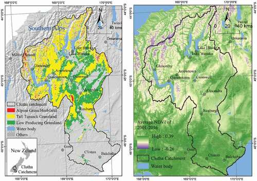
There are three principal grassland types in the study area covering a total of 10,562 km² (49.4%) of the catchment area: Alpine grassland (278 km², 1.3%), Tall Tussock grassland (6,406 km², 29.9%) and Low Producing grassland (3,878 km², 18.1%) (New Zealand Land Cover Database (LCDB-v4.1 2015). These three types are the principal grassland types in the rest of New Zealand and, in the study area, occur at average elevations of 1,574 m, 1,200 m and 640 m a.s.l., respectively. They are characterized by open, typically non-woody vegetation (see Table A1 for a detailed description). Low-producing grasslands, in contrast to alpine and tall tussock grasslands, can contain extensive elements dominated by non-native species and also may be subject to human interference and management in large parts of their distribution. The exact area of three grassland types were extracted from LCDB-v4.1 (Dymond et al. 2017; LCDB-v4.1 2015). The original LCDB data is in vector format. We converted it to a raster format in ArcGIS 10.1 using the MODIS NDVI pixels (250 m) as reference, so that the rasterized land cover data can match the NDVI time series by pixel.

2.2. NDVI and climate data

We used the Normalized Difference Vegetation Index (NDVI) derived from a near-daily MODIS dataset at 250 m spatial resolution to calculate annual time series of vegetation growth in the study area from 2001 to 2016 (Figure 1). The widely used NDVI is a useful and well established index to quantify temporal patterns in growth of grassland (Whittington et al. 2015; Xin et al. 2015; Leblans et al. 2017; Wilsey, Martin, and Kaul 2018). It ranges from −1 to 1 with higher values indicating higher biomass production activity and is calculated as

(1) $NDVI=\frac{\left(NIR-Red\right)}{\left(NIR+Red\right)}$(1)

where “NIR” and “Red” stand for the reflectance in the near infrared band and in red band, respectively. A 5-day maximum value composite was created from the near-daily NDVI time series to eliminate the noise due to high frequency of cloud/snow coverage in the raw data (Fontana et al. 2008).

Daily climate data was obtained from the Virtual Climate Station Network (VCSN) (NIWA Data: https://data.niwa.co.nz). VCSN is a gridded dataset at 0.05 degree latitude and longitude resolution covering the New Zealand land area. Each point of this VCSN grid provides daily climatic values, which are calculated through interpolation from actual climate station data (Tait, Sturman, and Clark 2012). For this study, climate data for the time period from 1 July 2000 to 30 June 2016 was extracted to coincide with the period of NDVI time series used here.

Eight daily climatic factors were chosen as explanatory variables and potential drivers in spatial and temporal variation in NDVI: soil temperature at 10 cm depth at 9 am (ETmp), mean sea level pressure (MSLP), rainfall (Rain), relative humidity (RH), solar radiation (Rad), maximum temperature (Tmax), minimum temperature (Tmin) and wind speed (Wind) (Figure A4). For the analyses of potential climate correlates of NDVI trends, the MODIS NDVI time series (250 m) was resampled at the 0.05 degree grid resolution of the VCSN climate grid.

2.3. Phenology indices

Growth phenology, i.e. the annual timing of the start, peak and end of biomass production in the grasslands was characterized using five phenological indices calculated from the NDVI time series for each pixel for each year (Table 1). We used the TIMESAT 3.3 tool with asymmetric Gaussian functions on the Matlab R2013b platform (Jonsson and Eklundh 2004) (http://web.nateko.lu.se/timesat/timesat.asp?cat=0, visited on 4 June 2020) to smooth the NDVI time series so as to derive the five indices from the NDVI time series.

Table 1. The five indices used to quantify growing season phenology in this study. The mDOY is the modified day of year, where mDOY 1 is 1st July of last year and mDOY 365 is 30th June of this year

No	Index	Abbreviation	Description
1	Start of season	SOS	Start of the growing season: the day where 50% of the year’s peak NDVI is reached for the first time, described by mDOY.
2	End of season	EOS	End of the growing season: the day at which NDVI falls under 50% of the peak NDVI, described by mDOY.
3	Length of season	LOS	Length of growing season: the time period in days between start and end of season, described by days.
4	Peak of season	POS	The peak of growing season, the day when the peak NDVI is reached, described by mDOY.
5	Peak day NDVI	P-NDVI	The fitted NDVI value on the day of the Peak of season

There are three smoothing functions in TIMESAT, namely Savitzky-Golay, Asymmetric Gaussian and Double Logistic. The Savitzky-Golay method is “over-sensitive” to inter-annual changes in NDVI time series (Fontana et al. 2008; Tan et al. 2011), and a large number of pixels in our data did not return any results from Savitzky-Golay function. The Asymmetric Gaussian and the Double Logistic functions returned the similar estimates for the five phenology indices. However, using the Double Logistic smoothing function resulted in more “no result” pixels than the Asymmetric Gaussian method. Other studies also demonstrated that the Asymmetric Gaussian function is more reliable when applied to data from mountainous environments (Tan et al. 2011; Beck et al. 2006; Li et al. 2017) and this function was therefore chosen here. The Asymmetric Gaussian method in TIMESAT 3.3 is a Gaussian type of function:

(2) $\mathrm{g}\left(\mathrm{t};x_1;x_2;x_3;x_4;x_5\right)=\left\{\begin{array}{c}exp\left[-{\left(\frac{t-x_1}{x_2}\right)}^{x_3}\right]\left(t>x_1\right)\\ exp\left[-{\left(\frac{x_1-t}{x_4}\right)}^{x_5}\right]\left(t<x_1\right)\end{array}\right.$(2)

In this function, t is the independent time variable; x₁ refers to the time when NDVI reaches maximum (or minimum); x₂ and x₃ determine the width and flatness of the right side of the fitted curve, while x₄ and x₅ determine the left side (for a detailed description see Eklundha and Jönsson (2017).

As expected for the southern hemisphere, annual growing seasons range from winter (July) 1 year to winter (July) the next year. Therefore, we used a modified day of year (mDOY) to describe a growing year from 1 July (day 1) to 30 June the next year (day 365) and to quantify the key stages in an annual growth cycle (Figure 2). The peak of season (POS) is defined as the day when the highest smoothed NDVI was reached. The difference between the peak NDVI and the base level (the mean of the two lowest smoothed NDVIs before and after POS in a year) is the “seasonal amplitude” of each year. In TIMESAT 3.3, we configured the seasonal amplitude at a 50% threshold which means the start of season (SOS) is defined as the day on which NDVI has increased by 50% of the seasonal amplitude from the left/lowest NDVI in each year. Similarly, the end of season (EOS) is the day on which NDVI has decreased by 50% of the seasonal amplitude after the peak of season in each year (Figure 2). The number of days between SOS and EOS is taken as the length of season (LOS).

Figure 2. Calculation of five phenological indices. Taking one pixel (see its location in the inset map) from the 16-year NDVI time series for example: the blue line is the raw NDVI data. The black curve is the asymmetric Gaussian function fitted values. Growing phenological indices were derived from the fitted values. Inset shows how the five phenological indices were calculated. SOS = Start of season, EOS = end of season, LOS = length of season, POS = peak of season, P-NDVI = peak day NDVI. We used a modified day-of-year (mDOY) to describe growth phenology in the southern hemisphere. A growing year starts from 1st July of last year and ends on 30th June of this year (mDOY 1 = 1st July of last year, mDOY 365 = 30st June)

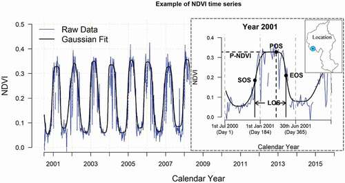
Table 2. Summary statistics (average, standard deviation) of the five phenological indices for the three grassland types for the study period 2001–2016. mDOY refers to the modified day of year with mDOY = 1 being 1^st July (see Table 1 and methods)

Phenological Index	Alpine		Tall Tussock		Low Producing
	Mean	SD.	Mean	SD.	Mean	SD.
Start (SOS, mDOY)	149.9	31.96	119.4	28.10	93.4	24.76
End (EOS, mDOY)	313.6	23.75	314.1	21.34	275.3	45.86
Length (LOS, days)	163.7	39.82	194.7	32.49	181.9	40.47
Peak (POS, mDOY)	233.8	20.27	219.7	19.92	182.7	31.90
Peak NDVI (P-NDVI)	0.33	0.109	0.47	0.078	0.59	0.088

Other parameters and settings in TIMESAT were determined from sensitivity analyses and include: Spike = 2, Number of envelopes = 3, Adaptation = 3. The “Spike = 2” setting indicates that outliers in the annual NDVI dataset are detected and removed based on the STL method (Seasonal Trend decomposition by LOESS). The setting of “Envelopes = 3” indicates that two iterations of upper envelope fitting were applied. The “Adaptation = 3” setting indicates the strength of envelope adaptation, which ranges from 1 (no adaptation) to 10 (strongest adaptation), indicating the degree of how close the fitted curve is to the envelope (Eklundha and Jönsson 2017). The more times the envelope is applied, and the stronger the adaptation, the higher the weight allocated to the high values of NDVI in function fitting.

2.4. Temporal trends and climate correlation analysis

The temporal trend of the five annual phenological indices over the 16-year study period was calculated for each MODIS NDVI pixel. This trend was quantified as the slope (β) of an ordinary least squares (OLS) regression model of phenological index against year for each pixel with positive slopes indicating a trend toward later season start/end/peak or longer season length. Because of spatial autocorrelation, the assumption of independence in OLS models might be violated if we use the phenological indices from all the pixels in one grassland type against year; additionally, we aim to depict the spatial variation of the temporal trend in the study area. Thus, the temporal trend was analyzed by pixel. For each grassland type, the median of all pixels of that grassland type and the pixels with the maximum and minimum slope were identified (Table 3). An ANOVA test was used to assess the significance of the trend over the 16 discrete years and the median slope was calculated for only the pixels with a significant (p < 0.05) trend (column Med* in Table 3).

Table 3. Temporal trends of five phenological indices during the study period 2001–2016. We calculated the OLS models of phenological indices against year for each single MODIS pixel, so each pixel has its own temporal trends quantified by the estimated values (slopes) of OLS models. The median (med) and extremes (max, min) are based on individual pixels in each grassland type, and the med* is the median of those pixels which showed a significant temporal trend (p < 0.05)

Phenological index	Grassland type	Med	Max	Min	Med*
Start (SOS, days/year)	Alpine	−0.72	2.43	−5.73	−2.10
	Tall Tussock	−0.60	5.80	−6.83	−1.64
	Low Producing	−0.88	10.82	−11.99	−1.47
End (EOS, days/year)	Alpine	−0.45	5.27	−4.60	−1.35
	Tall Tussock	−0.04	5.76	−6.48	1.36
	Low Producing	−0.04	12.07	−9.03	−0.71
Length (LOS, days/year)	Alpine	0.32	9.76	−3.99	2.81
	Tall Tussock	0.52	9.14	−6.05	2.73
	Low Producing	0.71	12.65	−10.69	2.56
Peak (POS, days/year)	Alpine	−0.63	1.98	−3.05	−1.54
	Tall Tussock	−0.32	4.11	−4.41	−1.34
	Low Producing	−0.66	10.26	−9.00	−2.24
Peak NDVI (P-NDVI, 10^−2/year)	Alpine	0.05	0.82	−1.24	0.24
	Tall Tussock	0.02	1.61	−1.49	0.16
	Low Producing	−0.04	2.54	−1.90	−0.20

The relationship between each growth phenology index and each climate variable was quantified using Pearson Correlation Coefficient (PCC). PCC ranges from −1 to 1, indicating negative to positive covariance of two variables. Correlation coefficients were calculated for all pairs of phenological index and each climatic factor in each grassland type for each VCSN pixel. The original daily VCSN climate data was transformed to seasonal and annual averages; winter and spring averages (June to November) were correlated with the start of season, spring and summer averages (September to February) with Peak of season, and summer and autumn averages (December to May) were correlated with for the End of season. Annual averages of the climatic variables were correlated with Length of season and Peak NDVI. The standardized correlation analyses and significance tests were conducted in R 3.5.3 with the package “stats” (R Core Team 2020).

3. Results

3.1. Spatial patterns in growth phenology

The start of growing season (SOS) during the study period occurred on average earliest in low-producing grasslands (modified Day of Year = 93.4 and latest in alpine grasslands (mDOY = 149.9; Table 2). There was considerable spatial variation in the start date of the growing season across the study area (Figure 3); This variation reflects the distribution of the three grassland types but also a west-to-east and high-to-low elevation trend of earlier start dates to the growing season.

Figure 3. The averages of phenological indices for the time period of 2001–2016. The start (a), peak (b) and end (c) days of growing season were described by a modified day of year (mDOY, which begins on 1st July of last year and ends on 30th June in this year). The length (d) of season was in units of days. The peak NDVI (e) ranged from 0.1–0.8 with higher values indicating more active vegetation

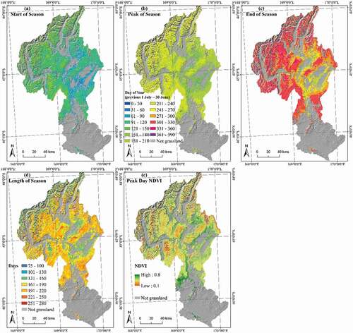
The end of the growing season (EOS) occurred in mid-autumn in both Alpine and Tall Tussock grasslands (313.6, 314.1 mDOY), while in Low Producing grassland EOS happened about one month earlier (275.3 mDOY) (Table 2). Within one grassland type (Tall Tussock) there was an obvious elevational differentiation in EOS in montane regions, where at higher elevations the growing season ended later than at lower elevations (Figure 3(c)).

The Tall Tussock grassland type had the longest growing season (LOS, 194.7 days) and Alpine grasslands the shortest (163.7 days) (Table 2). Overall, growing season length ranged from 75.9 to 278.1 days across the study area (Figure 3(d)). Most grasslands at higher elevation showed a shorter season length of c. 100 days, while in the lower montane grasslands season length could reach up to 220 days. In contrast, lowland grasslands in the central and eastern parts of the catchment, tended to have a shorter growing season at lower elevation, especially the Low Producing grasslands (often 131–160 days).

Low Producing grasslands reached their growing season peak day (POS) in early summer (average 182.7 mDOY), with Tall Tussock grasslands reaching their peak growth c. one month later (219.7 mDOY) and Alpine grasslands later still at 233.8 mDOY (Table 2). The peak growth day in three grassland types showed again an elevational spatial pattern of later peak days with increasing elevation (Figure 3(b)). Overall, all grassland types reached their POS during the summer months, apart from some grasslands in the eastern lowlands (mostly low-producing grasslands) which reached POS in late spring, possibly as a consequence of anthropogenic intervention.

The mean NDVI on the peak day (P-NDVI) ranged from 0.33 (Alpine) to 0.47 (Tall Tussock) and to 0.59 (Low Producing) with spatial patterns (Figure 3(e)) indicating the expected patterns of overall decreasing vegetation activity with increasing elevation.

3.2. Temporal trends in growth phenology 2001 – 2016

The start of the growing season (SOS) showed an advancing trend (i.e. earlier start) in over 85% of pixels in all three grassland types (Figure 4), with a median of a 0.72, 0.60 and 0.88 days/year earlier start in Alpine, Tall Tussock and Low Producing grasslands, respectively (Table 3 and Figure A1). While the vast majority of pixels showed an advancing trend in start of season, the low-producing grasslands typically showed the strongest trend with most pronounced shifts toward an earlier start of the growing season (Table 3, Figure 5(a)).

Figure 4. The distributions of the trends in each growth phenological index in each grassland type. ALP: Alpine grassland; TSK: Tall Tussock grassland; LPG: Low Producing grassland. The dotted vertical line in each panel separates the positive (red) and negative (blue) trends. The darker colored region indicates the significant (p < 0.05) trends. The proportion values in each panel show the percentages of positive/negative trends in all pixels, and the percentages in round brackets are the significant (p < 0.05) proportions of pixels

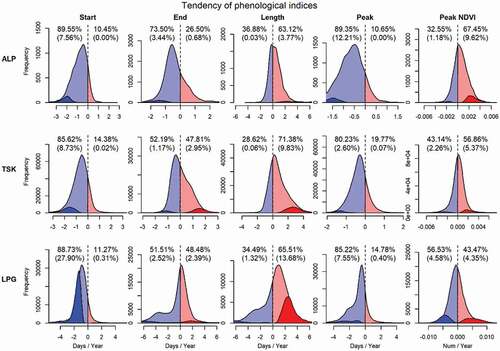
Figure 5. Temporal trends in the five growth phenological indices in the past 16 years (2001–2016). For start (a), End (b), Peak (c) and length (d) of season, the red (p ≤ 0.05) and coral (p > 0.05) colors represent the grassland with positive phenological trends (delayed start, end and peak of season, or prolonged length of season), and the blue (p ≤ 0.05) and turquoise (p > 0.05) colors illustrate the grassland with negative phenological trends (advanced start, end and peak of season, or shortened length of season). For peak NDVI (e), the green regions show an increasing trend in NDVI and dark-green color indicates significant, while the yellow areas show a decreasing trend in NDVI and brown color means significant

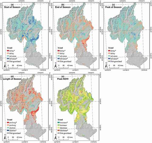
The end of growing season (EOS) occurred earlier in 73.5% of pixels in the Alpine grassland with a median of 0.45 days earlier per year. However, there was hardly a temporal trend of EOS in Tall Tussock and Low Producing grasslands (Figure 4 and Table 3); c. 50% of pixels in these two types showed an advanced and delayed end of season respectively. Tall Tussock grasslands, in particular in the eastern part of the catchment, showed the most pronounced trend toward a later end of the growing season (Figures 4, 5(b)).

A trend toward a longer growing season was observed for c. two-thirds of pixels in all three grassland types (Figure 4), with a median of 0.32 (Alpine), 0.52 (Tall Tussock) and 0.71 (Low Producing) days of increased season length per year respectively (Table 3). A significant trend toward a longer season typically occurred in Tall Tussock and Low Producing grasslands in eastern parts of the catchment (Figure 5(d)).

The peak growth day of the season (POS) occurred earlier in over 80% of the area of all grassland types (Figure 4) with a trend −0.63, −0.32 and −0.66 days earlier per year in Alpine, Tall Tussock and Low Producing grassland (Table 3). A significant trend toward an earlier peak day was mostly found in Alpine grassland at high elevation, as well as in Low Producing grassland at low elevation, but was hardly found in Tall Tussock grassland (Figure 5(c)).

The peak day NDVI (P-NDVI) showed an increasing trend in both Alpine and Tall Tussock grasslands(0.05 × 10⁻² and 0.02 × 10⁻² NDVI/year at median), while a declining trend was observed in Low Producing grassland (−0.04 × 10⁻² NDVI/year) (Table 3). There is no regular spatial pattern of the trend of P-NDVI in the study area (Figure 5(e)).

3.3. Climatic correlates of growth phenology

The start of season (SOS) was strongly correlated with atmospheric pressure (MSLP) and rainfall (Rain) in the winter–spring months (Table 4, Figure A2). When winter–spring MSLP was higher, the growing season started significantly earlier in 78% of Alpine grasslands, 64% of Tall Tussock grasslands and 25% of Low Producing grassland areas (Figure A2, Table 4). For those pixels which showed a significant positive relationship between start of season and rainfall (e.g. 21% of Alpine grassland pixels, there was 0.14 day earlier in the start of the season per mm of winter-spring rainfall decrease (Table 4). For 26% of Tall Tussock grassland and 23% of Low Producing grassland SOS was a 0.16 day earlier per mm 1 mm rainfall decrease, respectively (Table 4).

Table 4. Correlations between the five phenological indices and eight climatic factors. Values indicate the average slope (β) of OLS model of the pixels showing a significant linear relationships (t-test p < 0.05), and the percentages under the slopes indicate the proportions of the pixels in each grassland type showing a significant correlation

Index	Grass Type	ETmp	MSLP	Rad	Rain	RH	TMax	Tmin	Wind
Start SOS (days /unit)	Alp	−17.65	−3.35	−0.43	0.14	−4.71	−4.46	5.82	4.02
		1%	78%	1%	21%	2%	2%	1%	1%
	Tsk	−23.58	−3.05	−0.09	0.16	0.91	4.62	7.50	−13.20
		3%	64%	4%	26%	3%	1%	1%	4%
	Lpg	−17.49	−2.25	−0.06	0.16	4.95	−3.09	4.32	−16.04
		8%	25%	9%	23%	4%	3%	5%	8%
End EOS (days /unit)	Alp	8.15	1.80	0.05	0.10	−3.80	−6.20	3.97	25.10
		16%	2%	29%	2%	2%	1%	18%	4%
	Tsk	12.23	NA	0.04	0.35	−4.25	−2.56	2.83	28.79
		19%	0%	16%	2%	4%	<1%	7%	2%
	Lpg	−33.43	1.76	0.01	0.46	8.17	−3.39	4.86	13.27
		6%	7%	4%	32%	4%	2%	1%	4%
Length LOS (days /unit)	Alp	19.54	10.14	0.02	−0.04	5.23	−2.99	−8.53	21.94
		5%	11%	1%	1%	2%	1%	2%	5%
	Tsk	36.42	10.65	0.04	−0.05	−1.50	−3.07	−7.58	37.36
		9%	13%	1%	2%	7%	<1%	4%	12%
	Lpg	−5.35	11.44	−0.02	0.18	−3.11	1.64	−0.09	24.06
		10%	16%	3%	15%	2%	1%	6%	11%
Peak Day POS (days /unit)	Alp	−10.34	−2.10	0.07	0.13	−2.61	4.38	−0.30	18.48
		1%	1%	13%	4%	2%	2%	2%	4%
	Tsk	−12.67	3.68	0.05	0.15	−2.31	1.26	−6.43	25.42
		3%	<1%	5%	11%	5%	<1%	6%	1%
	Lpg	−10.87	−1.25	0.02	0.28	0.04	−2.54	−1.34	−1.87
		3%	3%	1%	40%	2%	1%	3%	3%
P-NDVI (1/unit)	Alp	−1.32 E-02	1.15 E-02	2.23 E-05	5.37 E-06	−6.68 E-04	3.58 E-03	−4.12 E-04	−1.81 E-03
		6%	26%	1%	5%	6%	16%	3%	2%
	Tsk	−1.01 E-02	5.66 E-03	−5.60 E-05	1.87 E-04	8.72 E-03	2.94 E-03	9.56 E-03	−5.32 E-02
		14%	9%	3%	7%	30%	17%	7%	12%
	Lpg	−1.32 E-02	−4.38 E-03	−4.54 E-05	2.23 E-04	1.22 E-02	−4.63 E-03	1.22 E-02	−6.78 E-02
		9%	6%	5%	19%	28%	4%	11%	16%

Abbreviations: ETmp: 10 cm earth temperature [°C], MSLP: mean sea level pressure [hPa], Rad: solar radiation [MJ/m²/day], Rain: rainfall [mm], RH: relative humidity [%], Tmax, Tmin: maximum, minimum temperature [°C], Wind: wind speed [m/s]. Alp: Alpine grassland, Tsk: Tall Tussock grassland, Lpg: Low Producing grassland.

Timing of the end of the growing season (EOS) was primarily correlated with four climatic factors: soil temperature (ETmp), radiation (Rad), rainfall (Rain) and minimum temperature (Tmin). In 16% of Alpine grassland, and in 19% of Tall Tussock grassland in the east of the catchment (Figure A2), the end of the growing season happened 8.15 and 12.23 days earlier per 1°C lower soil temperature (Table 4). In c. Alpine grassland (29%), and in parts of the Tall Tussock grasslands (16%) EOS was significantly advanced by 0.04–0.05 days per 1 MJ/m²/day radiation decrease during summer-autumn. The end of the growing season showed a significant positive relationship with rainfall in 32% of Low Producing grassland areas with 0.46 days earlier per mm rainfall decrease during summer-autumn (Figure A2). Particularly in Alpine grasslands (18% significant), the end of the season was advanced by 3.97 days per 1°C lower minimum temperature (Tmin) in the summer-autumn months.

Length of growing season (LOS) was significantly positively correlated with annual mean atmospheric pressure (MSLP) in 11% of Alpine grassland, 13% of Tall Tussock grassland and 16% of Low Producing grassland (Table 4) and with annual rainfall in 15% of Low Producing grasslands with a 0.18 days longer season per mm annual rainfall increase. A significantly positive relationship between season length and wind speed was found in 12% of Tall Tussock grassland and 11% of Low Producing grassland mostly in north-eastern parts of the catchment (Figure A2).

The peak day of the growing season (POS) was mostly correlated with solar radiation (Rad) or rainfall (Rain) in the spring-summer months. In 13% of Alpine grassland areas, the peak day happened 0.07 days earlier per MJ/m²/day spring-summer solar radiation decrease (Table 4). Significant positive relationships between POS and rainfall were found in 11% of Tall Tussock and 40% of low-producing grasslands with a 0.15 and 0.18 days earlier peak day per mm spring-summer rainfall decrease.

Peak annual NDVI (P-NDVI, i.e. the NDVI measured on the peak day) was positively correlated with relative humidity (RH) in 30% of Tall Tussock grassland and 28% of Low Producing grassland (Table 4). In 26% of Alpine grassland, P-NDVI showed a positive correlation with atmospheric pressure (MSLP). In 19% of Low Producing grassland, P-NDVI showed an increasing trend as radiation increased.

Overall, there was considerable spatial variation in the direction and strength of the relationships between the phenological indices and individual climatic factors investigated here (Figure A2). The strongest trends were observed for the start of the season which was often correlated with atmospheric pressure and precipitation changes during winter-spring, and for the end of season which was correlated with air temperature and solar radiation in summer-autumn. As only a limited number of climatic factors was investigated and no interactions between climate factors and between climate and anthropogenic activities were considered these trends are meant to show correlations but do not necessarily show a functional or causal relationship.

4. Discussion

4.1. Current shifts of growth phenology in grasslands

There is growing evidence that the timing of key growth stages in grasslands worldwide has experienced recent shifts with grasslands being amongst the best documented biomes for such shifts (Xin et al. 2015; Zhu and Meng 2015; Yu et al. 2017). A long-term observation on the Tibetan Plateau showed advanced spring leafing in alpine grassland during a recent period of climate change (Zhou et al. 2014). A three-year experiment in Minnesota, USA showed that the timing of spring green-up was sensitive to warming climatic conditions, but senescence was less clearly related to warmer temperatures (Whittington et al. 2015). Extended growing seasons were observed in Icelandic subarctic grasslands during the period of 2013–2015, again being a response in a direction expected under the concurrent climate warming in the area (Leblans et al. 2017). In the Southern Hemisphere, advanced spring life cycle events were observed in a wide variety of plants in Australia and New Zealand (Chambers et al. 2013). Other studies in China, Europe and Canada (Ma and Zhou 2012; Chang et al. 2017; Cui, Martz, and Guo 2017) also demonstrated a trend toward both an earlier start and extended length of the growing season but a much less pronounced response in the timing of the end of the growing season, something which is corroborated by the results from our study.

A recent study in the Australian Alps showed that grassland ecosystems exhibited an earlier start, a later end and greater length of the growing season during the 2000–2014 period (Thompson and Paull 2017). In their study, the start of the growing season occurred on 125 mDOY at the highest elevation (1800–1999 m a.s.l.) and on 96 mDOY at lower elevations (1400–1599 m a.s.l.). In our study, the start of season at the similar altitude, occurred at 149 mDOY in Alpine grassland (1300–1900 m) and 119 mDOY in the Tall Tussock grassland (800–1600 m) on average. The end of growing season in the Australian Alps was 320–335 mDOY at 1400–1999 m elevation, while it was at 310–315 mDOY at similar altitude in New Zealand. Overall, the growing season in the New Zealand’s grasslands investigated here (160–200 days) might be about 40 days shorter than in Australian grassland (200–240 days), but comparisons of actual dates are difficult due to different approaches for defining start and end of the growing season.

The shifts in growth phenology observed in our study between 2001 and 2016 are identical in direction, but typically smaller in magnitude than those observed in comparable grassland ecosystems elsewhere. In our study, the growing season started earlier by 6.0–8.8 days/decade depending on grassland type over the 16-year study period. The timing of the end of the season showed no particular advancing or retreating trend in Tall Tussock and Low Producing grasslands, but a trend of 4.5 days earlier/decade in Alpine grassland. Growing season length was extended by a median of 3.2, 5.2 and 7.1 days/decade in Alpine, Tall Tussock and Low Producing grassland, respectively. In comparison, a study in the Qinghai-Tibetan Plateau showed a 6.0 days /decade earlier start of season, a 2.0 days/decade delay in the end of season and a 8.0 days/decade longer growing season in alpine grassland ecosystems over a period of 10 years (1999–2009) (Ding et al. 2013). A study in the Australian Alps reported the start of season had advanced to an earlier date by 9–10 days/decade, the end of season occurred 0–18 days later/decade and the length of season increased by 11–29 days/decade during 2000–2014 (Thompson and Paull 2017). A recent study in grasslands in China (Yu et al. 2017) observed a 2.8 days earlier of start of season/decade, a 2.8 days later of end of season/decade and 6.6 days longer growing season/decade. These results therefore indicate that New Zealand’s grassland ecosystems, in particular those at highest elevations, have experienced recent shifts in key growing stages comparable to other regions (earlier start, delayed end and generally longer growing seasons) but that the magnitude of these shifts was typically smaller than in other parts of the world.

4.2. The responses of growing phenology indices to climate change

There is evidence that increased temperature often coincides with an earlier start and an extended length of the growing season in grasslands (Ma and Zhou 2012; Xia and Wan 2012). Likewise, shifting precipitation and drought patterns have also been shown to coincide with shifts in the start of the growing season in grassland ecosystems (Xia and Wan 2012; Cui, Martz, and Guo 2017). Overall, in our study, temperature affected growth phenology in considerably smaller areas than precipitation did (Table 4, Figure A2). Over the study period, air temperature increased significantly in the east and south and decreased in the mountainous western parts of the study area (Figure A3). These eastern, warming regions coincide with regions where an advanced start of season was most pronounced (Figure 5(a)). The precipitation in the catchment was relatively stable during the past 16 years, except for a substantial increase in the north-western mountain ridges, coinciding with areas of a later season end and later peak day (Figure 5). The locations with decreasing precipitation (Figure A3) typically also showed a shift toward an earlier start of the season (Figure 5(a)). Atmospheric pressure (MSLP) showed a positive temporal trend in the catchment during the study period (Figure A3), which also coincided with the trend of an advanced start of the growing season (Figure 5(a)). Phenological responses in plants are often reported to be correlated with large-scale atmospheric circulation oscillations (Schwartz 1992; Post and Stenseth 1999; Aasa et al. 2004), which in turn drive meteorological factors related to plants’ physiological functions. It is therefore not clear through which processes the surrogate factor air pressure might affect the start of the growing season. Overall, the start of growing season in New Zealand’s grasslands investigated here was strongly correlated with MSLP and modulated by precipitation and temperature.

Our results showed that the end of the growing season in Alpine and Tall Tussock grasslands was sensitive to temperature and solar radiation, and in Low producing grassland it was strongly correlated with precipitation. A recent study also showed that the end of season in specific grassland types was strongly correlated with temperature or precipitation depending on grassland type (Ren et al. 2018), and the end of season in Australian grasslands was not sensitive to altitude (Thompson and Paull 2017). In addition, we found some areas with a significant trend toward an earlier end of season in Low Producing grassland in central and eastern parts of the study area (Figure 5(b)). As the earlier end of season occurred in or near irrigation regions (Figure A5), grassland management practices are likely to significantly modify the timing of growing seasons in these areas.

The spatial distribution of the temporal trends in length of growing season (Figure 5d) was not consistently correlated with any single climate factor (Figure A2(c)). In general, our data showed that growing season length increased in most areas of the three grassland types, except the Tall Tussock grassland in the southern and the Low Producing grassland in the eastern portion of the catchment. The length of season was strongly correlated with atmospheric pressure and precipitation, and in some areas of Tall Tussock grassland season length was also correlated with wind speed. This indicates the length of season in these grasslands was more likely to be correlated with climatic factors that drive the start of the season rather than with those affecting the end of the season.

The timing of the peak of the growing season was mainly related to rainfall, especially in Low Producing grasslands, with higher rainfall coinciding with later peak growth. Other studies have also shown that in grassland ecosystems precipitation is a likely and expected key factor in the timing of peak growth (Cleland et al. 2006). The same study also found that increasing temperature can lead to an earlier growth peak of grassland species, likely a reflection of less water availability at higher temperatures. Our study showed the similar relationship: in large portions of the grasslands, a later peak of season was often significantly correlated with higher precipitation, but not with temperature (Figure A2(d)).

4.3. Limitations

This study focusses on phenological shifts in New Zealand’s indigenous grasslands at the ecosystem level (3 grassland types) and no attempt was made to include species-level information for the three grassland types in our analyses. The definitions of the three grassland types (LCDB-v4.1 2015) indicate that the three grassland types differ substantially in their functional make up both with and between types. The Alpine grassland (Alpine Grass/Herbfield) type comprises herbaceous cushion, mat, turf, rosette plants as well as lichens and abundant open ground with grasses often being only a minor component. For the Tall Tussock grassland type, there are two subtypes which are recognized but are not discernible in the land cover database used here (the indigenous snow tussock grasslands which generally occur in alpine/montane regions in South Island, and the red tussock grasslands which are usually found in lower elevations in both North Island and South Island. Due to the typically high proportion of indigenous plant cover in Tall Tussock grasslands, this type is probably the best representation of a New Zealand grassland type. The Low Producing grasslands in contrast, are a type defined by functional rather than ecological properties and include complex assemblages of native and exotic species. Though some pastoral lands containing exotic species are also classified as Low Producing grassland, the indigenous short tussock remnants of the South Island (and the study catchment) are a substantial element in this type.

Remote sensing methodologies enable us to derive and quantify growth phenology dynamics over much larger spatial extents and longer time periods than would be possible with field observations. The growth phenological metrics derived by remote sensing method in this study are the phenomena of land surface phenology (LSP), which is not equivalent to the concept of field observed phenology (Henebry and de Beurs 2013). Here we focussed on outlier detection and in order to extract reliable seasonal signals, curve regression and raw data modification were used to eliminate noisy and erroneous grid cells. There were originally 4,837, 102,448 and 61,102 pixels in Alpine, Tall Tussock and Low Producing grassland respectively. For each of the grassland types, there were 406, 2,172, and 4,639 pixels, respectively, that were excluded as erroneous pixels, due to failed criteria tests in TIMESAT. The proportion of removed pixels is less than 10% of the original number in each grassland type. Previous research has shown through field measurements validating MODIS data, that MODIS NDVI data provides accurate time series of growth phenology in grasslands (Fontana et al. 2008; Ganguly et al. 2010; Geng, Ma, and Wang 2016). Therefore, we are confident that the temporal patterns of growth phenology are accurately represented.

5. Conclusion

• Five growth phenological indices in New Zealand’s indigenous grasslands were derived from a MODIS NDVI time series for the time period 2001–2016 in order to identify recent shifts in the timing of growth in these grasslands. The start of growing season, defined here as the day at which 50% of the peak NDVI is first reached, occurred 7.2, 6.0 and 8.8 days per decade earlier in over 86% of Alpine, Tall Tussock and Low Producing grassland areas, respectively. The end of the growing season occurred 4.5 days per decade earlier in Alpine grasslands, but showed no significant temporal trend in the other two grassland types. The length of the growing season was extended by 3.2 (Alpine), 5.2 (Tall Tussock) and 7.1 (Low Producing) days per decade over the study period. In line with other grasslands elsewhere, the New Zealand grasslands investigated here also showed a pronounced temporal shift at the start but a much weaker shift at the end of the growing season with an overall increase in growing season length. Although comparisons with grasslands in other parts of the world are difficult due to differing (functional) species composition and environmental settings, it appears that the New Zealand grasslands investigated here show a shift in the same direction but at lower rates than grasslands elsewhere.

Overall, climatic variables related to air pressure and precipitation showed significant relationships with shifts in growth phenology over larger areas than climatic variables related to temperature did. However, these phenology-climate relationships varied substantially across space and between grassland types. The start of the season was significantly positively correlated with annual rainfall in a quarter of areas of Alpine and Tall Tussock grasslands. Higher precipitation delayed the peak and the end of the growing season in Low Producing grassland, but not in the other two types. Shifts in the length of the growing season were mainly correlated with changes in atmospheric pressure and rainfall over the study period. Our results highlight the differential responses of grassland ecosystems to a range of potential climatic drivers at different stages of the growing season further informing forecasts of ecosystem-level responses to future climate change. Our study demonstrates the usefulness of remotely sensed data for detecting and quantifying such responses in ecosystem processes over long time periods and large spatial extents.

Acknowledgements

Funding from Miss E. L. Hellaby Indigenous Grasslands Research Trust is gratefully acknowledged.

Disclosure statement

No potential conflict of interest was reported by the author(s).

Data availability statement

The processed MODIS NDVI data that support the findings of this study are available from the co-author Pascal Sirguey [email protected] upon reasonable request. The original MODIS imagery is available at https://modis.gsfc.nasa.gov/data/dataprod/.

The climate data (VCSN) that support the findings of this study are openly available in NIWA at https://data.niwa.co.nz.

Additional information

Funding

This work was supported by the Miss E. L. Hellaby Indigenous Grasslands Research Trust in August 2016.

Appendices

Figure A1 The trends of the five phenological indices in three grassland types during 2001–2016. The lines show the extremes and median of trends of five phenology indices in three grassland types. The red/blue solid lines are the most positive/negative tendency during the 16 years, and the dotted red/blue lines are for those two pixels. The gray line represents the median trend slopes in each scenario.

Irrigation regions in the study area (Clutha catchment). Data obtained from ministry for the environment, New Zealand (https://www.mfe.govt.nz/fresh-water/freshwater-guidance-and-guidelines/irrigated-land-new-zealand).

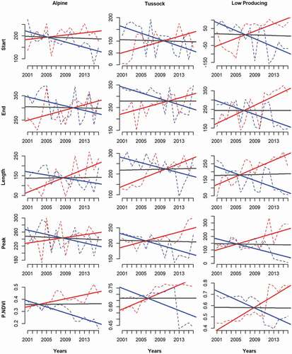
Figure A2. (Continued)

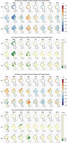
Figure A2. (Continued)

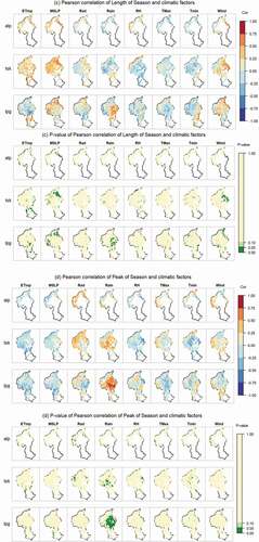
Figure A2. The spatial patterns of the correlations between annual growth phenological indices and climatic factors quantified by Pearson correlation coefficients (PCCs). The reddish colors represent positive relationships, while the blues mean negative correlations. The dark green colors indicate significant correlations (p < 0.05 in ANOVA test).

Abbreviations: ETmp, 10 cm earth temperature; MSLP, mean sea level pressure; Rad, solar radiation; Rain, rainfall; RH, relative humidity; Tmax, maximum temperature; Tmin, minimum temperature; Wind, wind speed; alp, Alpine grassland; tsk, Tall Tussock grassland; lpg, Low Producing grassland

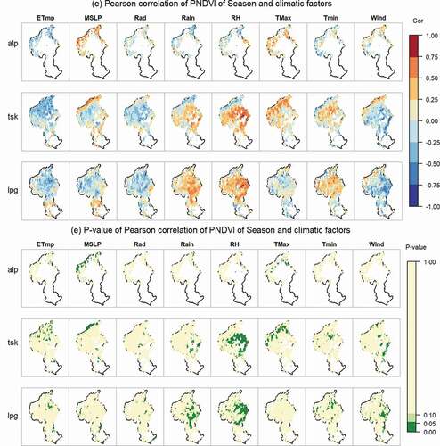
Figure A3. The trend of eight climate factors during the 2001–2016 study period. In each climate factor’s panel, the left map shows its trend of annual changes, and the map on the right shows the statistical significance (p-value) of its changing trend during 2001–2016.

Abbreviations: ETmp, 10 cm earth temperature (degC/year); MSLP, mean sea level pressure (hPa/year); Rad, solar radiation (MJ/m2/year); Rain, rainfall (mm/year); RH, relative humidity (%/year); Tmax, maximum temperature (degC/year); Tmin, minimum temperature (degC/year); Wind, wind speed (m/s/year)

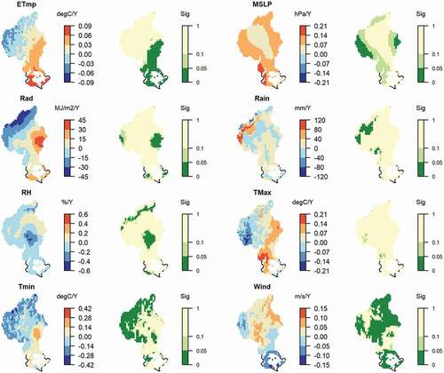
Figure A4. The averages of eight climatic factors in the Clutha river catchment in 2001–2016.

Abbreviations: ETmp: 10 cm earth temperature; MSLP: mean sea level pressure; Rad: solar radiation; Rain: rainfall; RH: relative humidity; Tmax, Tmin: maximum and minimum temperatures; Wind: wind speed

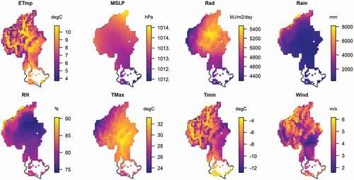
Figure A5. Irrigation regions in the study area (Clutha catchment). Data obtained from ministry for the environment, New Zealand

(https://www.mfe.govt.nz/fresh-water/freshwater-guidance-and-guidelines/irrigated-land-new-zealand)

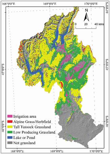
Table A1. Definitions of grassland types in LCDB v4.1

Class Name	Definition
Alpine Grass/Herbfield	Typically sparse communities above the actual or theoretical treeline dominated by herbaceous cushion, mat, turf, and rosette plants and lichens. Grasses are a minor or infrequent component, whereas stones, boulders and bare rock are usually conspicuous.
Tall Tussock Grassland	Indigenous snow tussocks in mainly alpine mountain-lands and red tussock in the central North Island and locally in poorly-drained valley floors, terraces and basins of both islands.
Low Producing Grassland	Exotic sward grassland and indigenous short tussock grassland of poor pastoral quality reflecting lower soil fertility and extensive grazing management or non-agricultural use. Browntop, sweet vernal, danthonia, fescue and Yorkshire fog dominate, with indigenous short tussocks (hard tussock, blue tussock and silver tussock) common in the eastern South Island and locally elsewhere.

References

- Aasa, A., J. Jaagus, R. Ahas, and M. Sepp. 2004. “The Influence of Atmospheric Circulation on Plant Phenological Phases in Central and Eastern Europe.” International Journal of Climatology: A Journal of the Royal Meteorological Society 24 (12): 1551–1564. doi:https://doi.org/10.1002/joc.1066.
- Beck, P. S. A., C. Atzberger, K. A. Hogda, B. Johansen, and A. K. Skidmore. 2006. “Improved Monitoring of Vegetation Dynamics at Very High Latitudes: A New Method Using MODIS NDVI.” Remote Sensing of Environment 100 (3): 321–334. doi:https://doi.org/10.1016/j.rse.2005.10.021.
- Blair, J., J. Nippert, and J. Briggs. 2014. “Grassland Ecology.” In: Monson R. (eds), Ecology and the Environment. The Plant Sciences 8. New York, NY: Springer. doi:https://doi.org/10.1007/978-1-4614-7501-9_14v
- Chambers, L. E., R. Altwegg, C. Barbraud, P. Barnard, L. J. Beaumont, R. J. M. Crawford, J. M. Durant, et al. 2013. “Phenological Changes in the Southern Hemisphere.” Plos One 8 (10): e75514. doi:https://doi.org/10.1371/journal.pone.0075514.
- Chang, J. F., P. Ciais, N. Viovy, J. F. Soussana, K. Klumpp, and B. Sultan. 2017. “Future Productivity and Phenology Changes in European Grasslands for Different Warming Levels: Implications for Grassland Management and Carbon Balance.” Carbon Balance and Management 12 (1). doi:https://doi.org/10.1186/s13021-017-0079-8.
- Chen, X. Q., S. An, D. W. Inouye, and M. D. Schwartz. 2015. “Temperature and Snowfall Trigger Alpine Vegetation Green-up on the World’s Roof.” Global Change Biology 21 (10): 3635–3646. doi:https://doi.org/10.1111/gcb.12954.
- Chmura, H. E., H. M. Kharouba, J. Ashander, S. M. Ehlman, E. B. Rivest, and L. H. Yang. 2019. “The Mechanisms of Phenology: The Patterns and Processes of Phenological Shifts.” Ecological Monographs 89 (1): e01337. doi:https://doi.org/10.1002/ecm.1337.
- Cleland, E. E., I. Chuine, A. Menzel, H. A. Mooney, and M. D. Schwartz. 2007. “Shifting Plant Phenology in Response to Global Change.” Trends in Ecology & Evolution 22 (7): 357–365. doi:https://doi.org/10.1016/j.tree.2007.04.003.
- Cleland, E. E., N. R. Chiariello, S. R. Loarie, H. A. Mooney, and C. B. Field. 2006. “Diverse Responses of Phenology to Global Changes in a Grassland Ecosystem.” Proceedings of the National Academy of Sciences of the United States of America 103 (37): 13740–13744. doi:https://doi.org/10.1073/pnas.0600815103.
- Cui, T. F., L. Martz, and X. L. Guo. 2017. “Grassland Phenology Response to Drought in the Canadian Prairies.” Remote Sensing 9 (12): 1258. doi:https://doi.org/10.3390/rs9121258.
- Day, N. J., and H. L. Buckley. 2013. “Twenty-five Years of Plant Community Dynamics and Invasion in New Zealand Tussock Grasslands.” Austral Ecology 38 (6): 688–699. doi:https://doi.org/10.1111/aec.12016.
- Ding, M. J., Y. L. Zhang, X. M. Sun, L. S. Liu, Z. F. Wang, and W. Q. Bai. 2013. “Spatiotemporal Variation in Alpine Grassland Phenology in the Qinghai-Tibetan Plateau from 1999 to 2009.” Chinese Science Bulletin 58 (3): 396–405. doi:https://doi.org/10.1007/s11434-012-5407-5.
- Dymond, J. R., J. D. Shepherd, P. F. Newsome, and S. Belliss. 2017. “Estimating Change in Areas of Indigenous Vegetation Cover in New Zealand from the New Zealand Land Cover Database (LCDB).” New Zealand Journal of Ecology 41 (1). doi:https://doi.org/10.20417/nzjecol.41.5.
- Eklundha, L., and P. Jönsson. 2017. “TIMESAT 3.3 With Seasonal Trend Decomposition and Parallel Processing—Software Manual.” Lund, Sweden: Lund University.
- Elzinga, J. A., A. Atlan, A. Biere, L. Gigord, A. E. Weis, and G. Bernasconi. 2007. “Time after Time: Flowering Phenology and Biotic Interactions.” Trends in Ecology & Evolution 22 (8): 432–439. doi:https://doi.org/10.1016/j.tree.2007.05.006.
- Fitter, A. H., and R. S. R. Fitter. 2002. “Rapid Changes in Flowering Time in British Plants.” Science 296 (5573): 1689–1691. doi:https://doi.org/10.1126/science.1071617.
- Fontana, F., C. Rixen, T. Jonas, G. Aberegg, and S. Wunderle. 2008. “Alpine Grassland Phenology as Seen in AVHRR, VEGETATION, and MODIS NDVI Time Series - a Comparison with in Situ Measurements.” Sensors 8 (4): 2833–2853. doi:https://doi.org/10.3390/s8042833.
- Ganguly, S., M. A. Friedl, B. Tan, X. Y. Zhang, and M. Verma. 2010. “Land Surface Phenology from MODIS: Characterization of the Collection 5 Global Land Cover Dynamics Product.” Remote Sensing of Environment 114 (8): 1805–1816. doi:https://doi.org/10.1016/j.rse.2010.04.005.
- Geng, L. Y., M. G. Ma, and H. B. Wang. 2016. “An Effective Compound Algorithm for Reconstructing MODIS NDVI Time Series Data and Its Validation Based on Ground Measurements.” Ieee Journal of Selected Topics in Applied Earth Observations and Remote Sensing 9 (8): 3588–3597. doi:https://doi.org/10.1109/jstars.2015.2495112.
- Henebry, G. M., and K. M. de Beurs. 2013. “Remote Sensing of Land Surface Phenology: A Prospectus.” In Phenology: An Integrative Environmental Science, edited by M. D. Schwartz, 385–411. Dordrecht: Springer Netherlands.
- Jentsch, A., J. Kreyling, J. Boettcher-Treschkow, and C. Beierkuhnlein. 2009. “Beyond Gradual Warming: Extreme Weather Events Alter Flower Phenology of European Grassland and Heath Species.” Global Change Biology 15 (4): 837–849. doi:https://doi.org/10.1111/j.1365-2486.2008.01690.x.
- Jeong, S.-J., H. Chang-Hoi, H.-J. Gim, and M. E. Brown. 2011. “Phenology Shifts at Start Vs. End of Growing Season in Temperate Vegetation over the Northern Hemisphere for the Period 1982-2008.” Global Change Biology 17 (7): 2385–2399. doi:https://doi.org/10.1111/j.1365-2486.2011.02397.x.
- Jonsson, P., and L. Eklundh. 2004. “TIMESAT - a Program for Analyzing Time-series of Satellite Sensor Data.” Computers & Geosciences 30 (8): 833–845. doi:https://doi.org/10.1016/j.cageo.2004.05.006.
- Kharouba, H. M., J. Ehrlen, A. Gelman, K. Bolmgren, J. M. Allen, S. E. Travers, and E. M. Wolkovich. 2018. “Global Shifts in the Phenological Synchrony of Species Interactions over Recent Decades.” Proceedings of the National Academy of Sciences of the United States of America 115 (20): 5211–5216. doi:https://doi.org/10.1073/pnas.1714511115.
- Körner, C., and D. Basler. 2010. “Phenology Under Global Warming.” Science 327 (5972): 1461–1462. doi:https://doi.org/10.1126/science.1186473.
- LCDB-v4.1. 2015. “Land Cover Database Version 4.1.” The Land Resource Information Systems Portal and scinfo.org.nz, Accessed June 16. https://lris.scinfo.org.nz/layer/423-lcdb-v41-land-cover-database-version-41-mainland-new-zealand.
- Leblans, N. I. W., B. D. Sigurdsson, S. Vicca, Y. S. Fu, J. Penuelas, and I. A. Janssens. 2017. “Phenological Responses of Icelandic Subarctic Grasslands to Short-term and Long-term Natural Soil Warming.” Global Change Biology 23 (11): 4932–4945. doi:https://doi.org/10.1111/gcb.13749.
- Leong, M., and G. K. Roderick. 2015. “Remote Sensing Captures Varying Temporal Patterns of Vegetation between Human-altered and Natural Landscapes.” Peerj 3: e1141. doi:https://doi.org/10.7717/peerj.1141.
- Li, G. Y., G. H. Jiang, J. Bai, and C. H. Jiang. 2017. “Spatio-temporal Variation of Alpine Grassland Spring Phenological and Its Response to Environment Factors Northeastern of Qinghai-Tibetan Plateau during 2000-2016.” Arabian Journal of Geosciences 10 (22). doi:https://doi.org/10.1007/s12517-017-3269-5.
- Linkosalo, T., R. Hakkinen, J. Terhivuo, H. Tuomenvirta, and P. Hari. 2009. “The Time Series of Flowering and Leaf Bud Burst of Boreal Trees (1846-2005) Support the Direct Temperature Observations of Climatic Warming.” Agricultural and Forest Meteorology 149 (3–4): 453–461. doi:https://doi.org/10.1016/j.agrformet.2008.09.006.
- Ma, T., and C. G. Zhou. 2012. “Climate-associated Changes in Spring Plant Phenology in China.” International Journal of Biometeorology 56 (2): 269–275. doi:https://doi.org/10.1007/s00484-011-0428-3.
- Mark, A. F., B. I. P. Barratt, E. Weeks, and J. R. Dymond. 2013. “Ecosystem Services in New Zealand’s Indigenous Tussock Grasslands: Conditions and Trends.” In Ecosystem Services in New Zealand: Conditions and Trends, edited by J. R. Dymond, 1–33. Lincoln, New Zealand: Manaaki Whenua Press, Landcare Research.
- Menzel, A., T. H. Sparks, N. Estrella, E. Koch, A. Aasa, R. Ahas, K. Alm-Kubler, et al. 2006. “European Phenological Response to Climate Change Matches the Warming Pattern.” Global Change Biology 12 (10): 1969–1976. doi:https://doi.org/10.1111/j.1365-2486.2006.01193.x.
- Miller-Rushing, A. J., and R. B. Primack. 2008. “Global Warming and Flowering Times in Thoreau’s Concord: A Community Perspective.” Ecology 89 (2): 332–341. doi:https://doi.org/10.1890/07-0068.1.
- Morisette, J. T., A. D. Richardson, A. K. Knapp, J. I. Fisher, E. A. Graham, J. Abatzoglou, B. E. Wilson, et al. 2009. “Tracking the Rhythm of the Seasons in the Face of Global Change: Phenological Research in the 21st Century.” Frontiers in Ecology and the Environment 7 (5): 253–260. doi:https://doi.org/10.1890/070217.
- Murray, D. L. 1975. “Regional Hydrology of the Clutha River.” Journal of Hydrology (New Zealand) 14 (2): 83–98.
- Parmesan, C. 2006. “Ecological and Evolutionary Responses to Recent Climate Change.” Annual Review of Ecology, Evolution, and Systematics 37 (1): 637–669. doi:https://doi.org/10.1146/annurev.ecolsys.37.091305.110100.
- Piao, S. L., Q. Liu, A. P. Chen, I. A. Janssens, Y. S. Fu, J. H. Dai, L. L. Liu, X. Lian, M. G. Shen, and X. L. Zhu. 2019. “Plant Phenology and Global Climate Change: Current Progresses and Challenges.” Global Change Biology 25 (6): 1922–1940. doi:https://doi.org/10.1111/gcb.14619.
- Post, E., and N. C. Stenseth. 1999. “Climatic Variability, Plant Phenology, and Northern Ungulates.” Ecology 80 (4): 1322–1339. doi:https://doi.org/10.1890/0012-9658(1999)080[1322:CVPPAN]2.0.CO;2.
- R Core Team. 2020. “R: A Language and Environment for Statistical Computing.” R Foundation for Statistical Computing, Vienna, Austria. https://www.R-project.org/
- Ren, S. L., S. H. Yi, M. Peichl, and X. Y. Wang. 2018. “Diverse Responses of Vegetation Phenology to Climate Change in Different Grasslands in Inner Mongolia during 2000-2016.” Remote Sensing 10 (1). doi:https://doi.org/10.3390/rs10010017.
- Sala, O. E., F. S. Chapin, J. J. Armesto, E. Berlow, J. Bloomfield, R. Dirzo, E. Huber-Sanwald, et al. 2000. “Biodiversity - Global Biodiversity Scenarios for the Year 2100.” Science 287 (5459): 1770–1774. doi:https://doi.org/10.1126/science.287.5459.1770.
- Schwartz, M. (Ed.) 2013. “Phenology An Integrative Environmental Science (p. 564).” Dordrecht: Kluwer Academic Publishers.
- Schwartz, M. D. 1992. “Phenology and Springtime Surface-layer Change.” Monthly Weather Review 120 (11): 2570–2578. doi:https://doi.org/10.1175/1520-0493(1992)120<2570:passlc>2.0.co;2.
- Sun, Z., Q. Wang, Q. Xiao, O. Batkhishig, and M. Watanabe. 2015. “Diverse Responses of Remotely Sensed Grassland Phenology to Interannual Climate Variability over Frozen Ground Regions in Mongolia.” Remote Sensing 7 (1): 360–377. doi:https://doi.org/10.3390/rs70100360.
- Tait, A., J. Sturman, and M. Clark. 2012. “An Assessment of the Accuracy of Interpolated Daily Rainfall for New Zealand.” Journal of Hydrology (New Zealand) 51: 25–44.
- Tan, B., J. T. Morisette, R. E. Wolfe, F. Gao, G. A. Ederer, J. Nightingale, and J. A. Pedelty. 2011. “An Enhanced TIMESAT Algorithm for Estimating Vegetation Phenology Metrics from MODIS Data.” Ieee Journal of Selected Topics in Applied Earth Observations and Remote Sensing 4 (2): 361–371. doi:https://doi.org/10.1109/jstars.2010.2075916.
- Testa, S., K. Soudani, L. Boschetti, and E. B. Mondino. 2018. “MODIS-derived EVI, NDVI and WDRVI Time Series to Estimate Phenological Metrics in French Deciduous Forests.” International Journal of Applied Earth Observation and Geoinformation 64: 132–144. doi:https://doi.org/10.1016/j.jag.2017.08.006.
- Thackeray, S. J., P. A. Henrys, J. R. Deborah Hemming, M. S. Bell, S. B. Botham, P. Helaouet, P. Helaouet, et al. 2016. “Phenological Sensitivity to Climate across Taxa and Trophic Levels.”Nature 535 (7611): 241–245. doi: https://doi.org/10.1038/nature18608.
- Thompson, J. A., and D. J. Paull. 2017. “Assessing Spatial and Temporal Patterns in Land Surface Phenology for the Australian Alps (2000–2014).” Remote Sensing of Environment 199: 1–13. doi:https://doi.org/10.1016/j.rse.2017.06.032.
- Visser, M. E., and C. Both. 2005. “Shifts in Phenology Due to Global Climate Change: The Need for a Yardstick.” Proceedings of the Royal Society B-Biological Sciences 272 (1581): 2561–2569. doi:https://doi.org/10.1098/rspb.2005.3356.
- Vitasse, Y., C. Francois, N. Delpierre, E. Dufrene, A. Kremer, I. Chuine, and S. Delzon. 2011. “Assessing the Effects of Climate Change on the Phenology of European Temperate Trees.” Agricultural and Forest Meteorology 151 (7): 969–980. doi:https://doi.org/10.1016/j.agrformet.2011.03.003.
- Wardle, P. 2008. “New Zealand Forest to Alpine Transitions in Global Context.” Arctic Antarctic and Alpine Research 40 (1): 240–249. doi:https://doi.org/10.1657/1523-0430(06-066).
- Weeks, E. S., S. Waker, J. R. Dymond, J. D. Shepherd, and B. D. Clarkson. 2013. “Patterns of past and Recent Conversion of Indigenous Grasslands in the South Island, New Zealand.” New Zealand Journal of Ecology 37 (1): 127–138.
- Whittington, H. R., D. Tilman, P. D. Wragg, and J. S. Powers. 2015. “Phenological Responses of Prairie Plants Vary among Species and Year in a Three-year Experimental Warming Study.” Ecosphere 6 (10). doi:https://doi.org/10.1890/es15-00070.1.
- Wilsey, B. J., L. M. Martin, and A. D. Kaul. 2018. “Phenology Differences between Native and Novel Exotic-dominated Grasslands Rival the Effects of Climate Change.” Journal of Applied Ecology 55 (2): 863–873. doi:https://doi.org/10.1111/1365-2664.12971.
- Wolters, E., E. Swinnen, C. Toté, and S. Sterckx. 2018. “Spot-VGT Collection 3 Products User Manual, V1. 2. (p. 54)” In Flemish Institute for Technological Research (VITO). Belgium: Antwerp.
- Wright, K. W., K. L. Vanderbilt, D. W. Inouye, C. D. Bertelsen, and T. M. Crimmins. 2015. “Turnover and Reliability of Flower Communities in Extreme Environments: Insights from Long-term Phenology Data Sets.” Journal of Arid Environments 115: 27–34. doi:https://doi.org/10.1016/j.jaridenv.2014.12.010.
- Xia, J. Y., and S. Q. Wan. 2012. “The Effects of Warming-Shifted Plant Phenology on Ecosystem Carbon Exchange are Regulated by Precipitation in a Semi-Arid Grassland.” Plos One 7 (2). doi:https://doi.org/10.1371/journal.pone.0032088.
- Xin, Q. C., M. Broich, P. Zhu, and P. Gong. 2015. “Modeling Grassland Spring Onset across the Western United States Using Climate Variables and MODIS-derived Phenology Metrics.” Remote Sensing of Environment 161: 63–77. doi:https://doi.org/10.1016/j.rse.2015.02.003.
- Yu, L. X., T. X. Liu, K. Bu, F. Q. Yan, J. C. Yang, L. P. Chang, and S. W. Zhang. 2017. “Monitoring the Long Term Vegetation Phenology Change in Northeast China from 1982 to 2015.” Scientific Reports 7. doi:https://doi.org/10.1038/s41598-017-14918-4.
- Zhang, J. H., Q. F. Yi, F. W. Xing, C. Y. Tang, L. Wang, W. Ye, I. I. Ng, T. I. Chan, H. F. Chen, and D. M. Liu. 2018. “Rapid Shifts of Peak Flowering Phenology in 12 Species under the Effects of Extreme Climate Events in Macao.” Scientific Reports 8. doi:https://doi.org/10.1038/s41598-018-32209-4.
- Zhang, X. Y., M. A. Friedl, C. B. Schaaf, A. H. Strahler, J. C. F. Hodges, F. Gao, B. C. Reed, and A. Huete. 2003. “Monitoring Vegetation Phenology Using MODIS.” Remote Sensing of Environment 84 (3): 471–475. doi:https://doi.org/10.1016/s0034-4257(02)00135-9.
- Zhou, H. K., B. Q. Yao, W. X. Xu, X. Ye, J. J. Fu, Y. X. Jin, and X. Q. Zhao. 2014. “Field Evidence for Earlier Leaf-out Dates in Alpine Grassland on the Eastern Tibetan Plateau from 1990 to 2006.” Biology Letters 10 (8): 20140291. doi:https://doi.org/10.1098/rsbl.2014.0291.
- Zhu, L. K., and J. J. Meng. 2015. “Determining the Relative Importance of Climatic Drivers on Spring Phenology in Grassland Ecosystems of Semi-arid Areas.” International Journal of Biometeorology 59 (2): 237–248. doi:https://doi.org/10.1007/s00484-014-0839-z.