Aboveground biomass estimates over Brazilian savannas using hyperspectral metrics and machine learning models: experiences with Hyperion/EO-1

ABSTRACT

We investigated the potential of hyperspectral remote sensing to estimate aboveground biomass (AGB) over the Brazilian savannas (Cerrado), the second-largest source of carbon emissions in Brazil. For this purpose, a Hyperion/Earth Observing-1 (EO-1) image was collected in the dry season at the Ecological Station of Águas Emendadas (ESAE). In order to estimate the AGB, we evaluated the performance of five machine learning models (Classification and Regression Trees – CART; Cubist – CB, Partial Least Squares Regression – PLS; Random Forest – RF; and Support Vector Machine – SVM) and four sets of metrics (reflectance, narrowband vegetation indices – VIs; absorption band parameters; and the combination of these attributes). The lowest root mean square error (RMSE) was obtained for RF using VIs (29%) and a combination of metrics (28%). For VIs, RF differed from CUB, PLS and SVM at 5% significance level. From cross-validation results, the RMSE was 26.36% for grasslands, 35.04% for open savannas, and 24.85% for dense savannas. The RF model with VIs had the most stable predictive performance across the models, as indicated by small variations in RMSE from CART to SVM. The five most important ranked VIs in the RF model were the Normalized Difference Vegetation Index (NDVI), Pigment Specific Simple Ratio (PSSR), Enhanced Vegetation Index (EVI), Red Edge Normalized Difference Vegetation Index (RENDVI) and Structure Insensitive Pigment Index (SIPI). Most of their relationships with AGB were non-linear. The resultant AGB estimates showed consistent results with a vegetation cover map of the ESAE. Areas of the ESAE with AGB lower than 10 Mg.ha⁻¹ were coincident with the occurrence of grassland physiognomies (savanna grasslands and shrub savannas), while areas with AGB higher than 25 Mg.ha⁻¹ matched the occurrence of dense savanna physiognomies (woodland savanna and dense woodland savanna). Grassland areas showed larger values of coefficient of variation (CV) than areas of dense savannas. These first-hand results set a baseline of models and metrics for AGB modeling of savannas during the future transition from current sampling-type hyperspectral missions (< 10 km of swath) to large-coverage hyperspectral satellites (> 100 km of swath).

KEYWORDS:

• Hyperspectral remote sensing
• aboveground biomass (AGB)
• savannas
• Cerrado
• machine learning
• Hyperion/EO-1

1. Introduction

Savannas are composed of different proportions of woody and herbaceous physiognomies. They represent approximately 20% of terrestrial vegetation, contributing significantly to global carbon cycle (Sankaran et al. 2005; Grace et al. 2016; Muumbe et al. 2021). In Brazil, savannas are locally known as the Cerrado vegetation. As one of the world´s hotspots of biodiversity, the Cerrado is the second largest biome in the country after the Amazon forest (Myers et al. 2000; Sano, Ferreira, and Huete 2005; Liesenberg, Galvão, and Ponzoni 2007). Covering more than 200 million hectares in Brazil, the Cerrado has vegetation gradients that range from grasslands to woodlands, depending on several factors such as soil moisture, soil nutrients and rainfall (Ribeiro and Walter 1998; Oliveira-Filho and Ratter 2002; Felfili et al. 2008; Ferreira et al. 2011). This type of vegetation is well adapted to fire and to the marked seasonal differences in rainfall observed in the rainy and dry seasons (Ratter, Bridgewater, and Ribeiro 2006).

Only 55% of the Cerrado area is still covered by native vegetation (Sano et al. 2010; Bispo et al. 2020). The landscape is fragmented due to the effects of agricultural activities that affect the conservation of biodiversity. Because of the opening of new agricultural frontiers for soybean production, savanna-clearing rates have recently exceeded the rates of tropical forest conversion in the Amazon (Zalles et al. 2019; Souza et al. 2020). Consequently, the Cerrado is the second-largest source of carbon emissions in Brazil (De Miranda et al. 2014). This fact highlights the importance of monitoring its aboveground biomass (AGB). AGB is a major component of the terrestrial carbon cycle (Houghton, Hall, and Goetz 2009; Ribeiro et al. 2011; Bispo et al. 2020). Estimates of this biophysical parameter are also critical for supporting policies of ecosystem functioning conservation and climate change mitigation (Almeida et al. 2019).

Remote sensing is the major source of information for estimating AGB over large areas at the landscape, regional and global scales. However, in contrast to forest ecosystems, there is a paucity of research aimed at using remote sensing for estimating AGB of savannas (Braun, Wagner, and Hochschild 2018; Wessels et al. 2019; Forkuor et al. 2020). Examples in Brazil include the studies by Bitencourt et al. (2007), Miguel et al. (2015), Schwieder et al. (2018) and Bispo et al. (2020). In general, they used orbital multispectral and Synthetic Aperture Radar (SAR) data as well as airborne Light Detection and Ranging (LiDAR) observations to predict AGB over different test sites. As far as we know, none of the studies that included the Brazilian savannas investigated the potential of using hyperspectral data for this purpose. One of the reasons is the limited availability of hyperspectral data over this ecosystem. Considering the uncertainties of the AGB estimates observed in previous studies and the possibilities of launching large swath width hyperspectral missions, this investigation is important. Furthermore, more studies of AGB quantification are necessary to better understand the patterns of carbon emission in the Cerrado (Bispo et al. 2020).

The Hyperion/Earth Observing-1 (EO-1), launched in 2000, operated with 30 m spatial resolution in 196 radiometrically calibrated bands positioned in the 426–2395 nm range (Pearlman et al. 2003; Galvão, Souza, and Breunig 2019). The instrumental signal-to-noise ratio (SNR) was approximately 40 in the shortwave infrared (SWIR), which resulted in noisy images in this spectral interval. Because of its narrow swath width (7.7 km), the Hyperion was considered a sampling-mission type. In spite of being decommissioned in 2017, its historical data provide an opportunity for research studies as preparation for the new generation of hyperspectral sensors with larger swath width and better SNR than Hyperion (Jacon et al. 2017; De Oliveira, Galvão, and Ponzoni 2019).

Compared to multispectral sensors, hyperspectral instruments such as Hyperion provide a larger number of metrics for AGB estimates (Galvão, Souza, and Breunig 2019). For instance, because of the great number of bands of the imaging spectrometers, we can calculate dozens of narrowband vegetation indices (VIs) and absorption-band parameters (Toniol et al. 2017). These metrics can serve as input variables to predict AGB using different machine learning models and field inventory data. Machine learning models can provide more accurate estimates of AGB than regression models (Nunes and Gorgens 2016). The predictive power of the machine learning approaches should be therefore tested on the Brazilian savannas using hyperspectral data. Examples of models that can handle a great number of hyperspectral metrics include Classification and Regression Trees (CART), Cubist (CB), Partial Least Squares regression (PLS), Random Forest (RF) and Support Vector Machine (SVM).

In this study, we evaluated the performance of satellite hyperspectral data for estimating the AGB of savannas from central Brazil. The specific goals were 1) to determine the machine learning model having the lowest root mean square error (RMSE) for estimating AGB among CART, CB, PLS, RF and SVM; and 2) to analyze the performance of four sets of Hyperion/EO-1 metrics (reflectance, narrowband VIs; absorption band parameters; and the combination of these attributes) for this purpose. By indicating which types of metrics and models produce the best predictive performance, this hyperspectral study establishes a baseline for future investigations over the Cerrado using larger swath-width hyperspectral satellites than Hyperion.

2. Methodology

The main methodological steps for AGB estimates over the savannas are shown in the flowchart of Figure 1. The steps are detailed in the next sub-sections.

Figure 1. Methodology adopted to estimate aboveground biomass (AGB) over the savannas using different hyperspectral metrics and machine learning models

2.1. Selection of the study area

The Ecological Station of Águas Emendadas (ESAE), located in central Brazil, was selected as the study area because it has some of the most important Brazilian savanna physiognomies. The ESAE is a 10,000-ha protected area located close to the Brasília city in the Cerrado biome (Figure 2). The study area has well defined rainy (October to April) and dry (May to September) seasons with average values of annual precipitation and temperature of 1552 mm and 21°C, respectively (Jacon et al. 2017). Total precipitation during the dry season is very low (< 80 mm) and the altitude ranges from 1000 to 1200 m. The most important soil types are Latossolo Vermelho (Rhodic Acrustox in the U.S. Soil Taxonomy), Latossolo Vermelho-Amarelo (Typic Acrustox), and Gleissolos Háplicos (Aquox).

Figure 2. Location of the Ecological Station of Águas Emendadas (ESAE) in the Cerrado biome in Brazil. The 45 sample plots are indicated over the available vegetation map, adapted from GeoLógica/Ecotech (2009) and Jacon et al. (2017). The number of plots (n) per physiognomy is indicated between parentheses

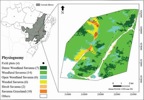
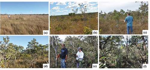
The ESAE has a well-defined gradient with increasing vegetation cover from grasslands to woodlands (Figure 3a-f). Based on the classification by Ribeiro and Walter (1998), savanna grasslands do not have trees (Figure 3a), while dense woodland savannas have more than 50% of vegetation cover (Figure 3f). There are also areas of riparian forests and Veredas, a linear-shaped physiognomy with palm trees (buritis; Mauritia flexuosa L.) along the streams. We did not model their AGB because they were not sampled in the field.

Figure 3. Areas representative of the (a) savanna grasslands; (b) shrub savannas; (c) wooded savannas; (d) open woodland savannas; (e) woodland savannas; and (f) dense woodland savannas

2.2. Fieldwork activities for AGB determination

During the dry season of 2015, we surveyed the floristic and structural attributes of 45 sample plots (20 m × 50 m) indicated in Figure 2. We measured the height of all trees and shrubs with diameter equal or larger than 5 cm at 30 cm from the ground. Because many trunks bifurcate close to the ground, the use of the 30-cm distance to measure the diameter is generally adopted in forest inventories of the Brazilian savannas (Felfili, Carvalho, and Haidar 2005). We used the allometric equation of Rezende et al. (2006) to determine the AGB of the plots, specifically the Model 1 for dry woody biomass (Eq. 1)(1) $AGB=-0.4913+0.0291\ast D{b}^2\ast Ht$(1) :

(1) $AGB=-0.4913+0.0291\ast D{b}^2\ast Ht$(1)

where AGB corresponds to individual aboveground biomass (kg); Db corresponds to the diameter measured at 30 cm from the ground (cm); and Ht corresponds to the total height (m). When describing the precision of this model, the authors reported a sampling error of 25.79%.

The strategy adopted over the grassland areas included the use of five polymerized vinyl chloride (PVC) quadrats (1 m × 1 m) distributed at 10-m spacing intervals within each transect (20 m × 50 m). We cut, collected and weighted the herbaceous material. A sample of 100 g was collected over each sub-plot. We transported this material to the laboratory for oven drying and for subsequent determination of total dry biomass. The samples were dried at 65°C during 48 hours to determine the fresh-to-dry weight relationship (Eq. 2)(2) $Md\left(f\right)=\frac{Mw\left(f\right)\ast Md\left(s\right)}{Mw\left(s\right)}$(2) :

(2) $Md\left(f\right)=\frac{Mw\left(f\right)\ast Md\left(s\right)}{Mw\left(s\right)}$(2)

where Md(f) corresponds to the total dry matter mass in the field (kg); Md(s) is the dry mass of the samples (kg) after oven drying; Mw(s) corresponds to the wet mass of the samples (kg); and Mw (f) refers to the total wet matter mass in the field (kg).

Tree height, basal area, and tree density increased from wooded savanna to dense woodland savanna (Table 1). The tallest trees ranged between 2 and 3 meters for these physiognomies. Shrub savannas and savanna grasslands did not have trees or shrubs with diameter greater than 5 cm.

Table 1. Structural-floristic attributes of the savanna physiognomies sampled in the field over the Ecological Station of Águas Emendadas (ESAE). Mean and standard deviation values are provided

Structural-floristic attributes	Savanna grassland	Shrub savanna	Wooded savanna	Open woodland savanna	Woodland savanna	Dense woodland savanna
Sample plots	10	2	6	6	14	7
AGB (Mg.ha^−1)	4.0 ± 0.7	5.8 ± 1.3	9.7 ± 3.4	14.1 ± 5.9	26.6 ± 6.9	34.5 ± 2.7
Mean height (m)	-	-	2.3 ± 1.3	2.5 ± 1.3	2.7 ± 1.6	3.0 ± 1.7
Basal area (m^2.ha^−1)	-	-	8.3 ± 1.6	11.7 ± 4.7	16.5 ± 2.2	22.0 ± 1.5
Density (ind.ha^−1)	-	-	1162 ± 273	1635 ± 394	2171 ± 475	2415 ± 388
Shannon–Wiener (H′)	-	-	3.14	3.30	3.35	3.28
Pielou (J)	-	-	0.78	0.81	0.79	0.79

A floristic survey was also performed in the field for the calculation of the Shannon–Weaver (H’) and Pielou evenness (J) indices. The floristic diversity, expressed by the H’ and J indices, was similar for dense woodland savanna, woodland savanna, open woodland savanna and wooded savanna (Table 1). The predominant species identified in the field vegetation inventory were Miconia Sp. (miconia – Melastomastaceae), Kielmeyera coriacea Mart. (pau-santo – Clusiaceae) and Sclerolobium paniculatum Vogel (carvoeiro – Fabaceae) over the dense woodland and woodland savanna areas; and Kielmeyera coriacea Mart., Dalbergia miscolobium Benth. (jacarandá do cerrado – Fabaceae) and Annona crassiflora Mart. (araticum – Annonaceae) over the open woodland and wooded savanna areas.

2.3. Hyperion data acquisition and pre-processing

The Hyperion image was collected over the ESAE during the dry season of 2014 (July 10) with a solar zenith angle of 49° and a pointing angle of 12°. After using an algorithm to reduce striping (Goodenough et al. 2003), we converted the at-sensor radiance data into surface reflectance images. For this purpose, the Fast Line-of-sight Atmospheric Analysis of Spectral Hypercubes (FLAASH) algorithm (Harris Geospatial Solutions, Inc., Melbourne, Florida) was applied over the data to reduce the effects of atmospheric scattering and absorption. Model parameters included a tropical atmosphere with a rural aerosol. The visibility was estimated using the 2-Band (K–T) method (Kaufman et al. 1997). To estimate atmospheric water vapor on a per-pixel basis, we selected the 1130-nm spectral feature. The FLAASH polishing algorithm removed spectral artifacts resulting from atmospheric correction.

After atmospheric correction, we excluded noisy bands associated with intervals of strong water vapor absorption (1400 and 1900 nm) and left 144 bands in the data analysis.

2.4. Selection of the hyperspectral metrics

We tested three types of hyperspectral data as input variables for the machine learning models: the reflectance of 144 Hyperion bands; 22 narrowband VIs; and 24 absorption band parameters. We also tested a combination of these 190 variables to build the models. To relate these variables to the field-measured AGB, we created polygons matching the sample plots recorded in the field using a Garmin Global Positioning System (GPS). We then extracted the mean values of each hyperspectral metric from the entire plot area.

The VIs of Table 2 are sensitive to changes in canopy structure (EVI, NDVI, VARI and VIG), biochemistry (ARI, CAI, CRI1, LWVI2, MCARI, MSI, NDII, NDLI, NDWI, PSRI, PSSR, SIPI and WBI) and physiology (PRI, RENDVI, REPI, RVSI and VOG). Some of them are sensitive to more than one vegetation parameter (Roberts, Roth, and Perroy 2012). Equations and references of the VIs are listed in Table 2.

Table 2. Narrowband vegetation indices (VIs) selected as input variables to the machine learning models for estimating aboveground biomass (AGB) over the savanna areas. ρ is the reflectance of the closest Hyperion bands to the original formulations (in nm)

Vegetation indices (VIs)			Equations	Reference
Structure	EVI	Enhanced Vegetation Index	2.5 × ((ρ864 − ρ660)/(ρ864 + 6 × ρ660 − 7.5 × ρ487 + 1))	Huete et al. (2002)
	NDVI	Normalized Difference Vegetation Index	(ρ864 − ρ660)/(ρ864 + ρ660)	Rouse et al. (1973)
	VARI	Visible Atmospherically Resistant Index	(ρ559 − ρ660)/(ρ559 + ρ660 – ρ487)	Gitelson et al. (2002a)
	VIG	Visible Green Index	(ρ559 − ρ660)/(ρ559 + ρ660)	Gitelson et al. (2002a)
Biochemistry	ARI	Anthocyanin Reflectance Index	(1/ ρ559) – (1/ ρ721)	Gitelson, Merzlyak, and Chivkunova (2001)
	CAI	Cellulose Absorption Index	100*[0.5*(ρ2032+ ρ2213)- ρ2102]	Daughtry (2001)
	CRI1	Carotenoid Reflectance Index 1	(1/ ρ510) – (1/ ρ550)	Gitelson et al. (2002b)
	LWVI2	Leaf Water Vegetation Index 2	(ρ1094 – ρ1205)/(ρ1094 + ρ1205)	Galvão, Formaggio, and Tisot (2005)
	MCARI	Modified Chlorophyll Absorption Ratio Index	[(ρ701- ρ671) – 0.2*(ρ701- ρ549)]* (ρ701/ ρ671)	Daughtry et al. (2000)
	MSI	Moisture Stress Index	(ρ1598)/ (ρ823)	Hunt and Rock (1989)
	NDII	Normalized Difference Infrared Index	(ρ823 − ρ1649)/ (ρ823 + ρ1649)	Hunt and Rock (1989)
	NDLI	Normalized Difference Lignin Index	[log(1/ρ1754) − log(1/ρ1680)]/[log(1/ρ1754) + log(1/ρ1680)]	Serrano, Peñuelas, and Ustin (2002)
	NDWI	Normalized Difference Water Index	(ρ854 − ρ1245)/ (ρ854 + ρ1245)	Gao (1996)
	PSRI	Plant Senescence Reflectance Index	(ρ681 – ρ498)/ρ752	Merzlyak et al. (1999)
	PSSR	Pigment Specific Simple Ratio	ρ803/ρ671	Blackburn (1998)
	SIPI	Structure Insensitive Pigment Index	(ρ803 − ρ467)/(ρ803 – ρ681)	Peñuelas, Baret, and Filella (1995)
	WBI	Water Band Index	ρ 905/ρ972	Peñuelas et al. (1997)
Physiology	PRI	Photochemical Reflectance Index	(ρ529 − ρ569)/(ρ529 + ρ569)	Gamon, Serrano, and Surfus (1997)
	RENDVI	Red Edge Normalized Difference Vegetation Index	(ρ752 − ρ701)/(ρ752 + ρ701)	Gitelson, Merzlyak, and Lichtenthaler (1996)
	REPI	Red Edge Position Index	L (maximum first derivative in the range 690–740)	Horler, Dockray, and Barber (1983)
	RVSI	Red-Edge Vegetation Stress Index	[(ρ712 + ρ752)/2] – ρ732	Merton and Huntington (1999)
	VOG	Vogelmann Red Edge Index	ρ742/ρ722	Vogelmann, Rock, and Moss (1993)

In addition to the reflectance of 144 bands and 22 VIs, we calculated four absorption band parameters (depth, width, area and asymmetry) from six spectral features using the Processing Routines in IDL for Spectroscopic Measurements (PRISM) (Sanches, Souza Filho, and Kokaly 2014). The routines use the continuum removal method to filter out features from the spectra before quantifying their parameters. Absorption band parameters from the following features were retrieved on a per-pixel basis: chlorophyll absorption band centered at 680 nm; leaf water spectral features positioned at 980 nm and 1200 nm; and lignin–cellulose absorptions located at 1700 nm, 2100 nm, and 2300 nm. Kokaly and Skidmore (2015) described each parameter and listed the equations used for their determination.

2.5. Machine learning models and validation

All statistical models were created using the R programming language (R Development Core Team 2021). We tested five models to estimate AGB using the caret R package (Kuhn 2008): CART, CUB, PLS, RF, and SVM. Details and examples of the use of these models can be found in Breiman (2001), Friedman (2002), Sibanda, Mutanga, and Rouget (2016), Basak, Pal, and Patranabis (2017), Almeida et al. (2019), and Rasanen et al. (2020). Four types of data were tested as predictors for each model: (i) the reflectance of 144 Hyperion bands; (ii) 22 narrowband VIs; (iii) 24 absorption band parameters; and (iv) all 190 variables combined.

For model training and validation, we employed a cross-validation with stratified random permutations from 100 repetitions. The stratification included data from all the AGB distribution during training. For this purpose, we considered five groups of 20th quantile intervals and obtained samples from each group to represent the whole AGB gradient. This means that the data were iteratively partitioned into training and validation datasets 100 times using 80% and 20% of the total samples (n = 45 samples), respectively. During each run, we obtained the RMSE, which was used to compare the models. This ensures confidence in the validation procedure. Therefore, the partition considered data distribution from grasslands to dense savannas to represent the whole AGB gradient during training. To calibrate the hyperparameters of each model, we employed 30 bootstrap iterations. A list of the hyperparameters of each model can be found in Kuhn (2008).

In order to visualize the variability of the AGB predictions from the best model, a predicted versus observed AGB plot was generated considering the out-of-sample (OOS) estimates from 100 repetitions. The mean and standard deviation (SD) were plotted for each sample. A plot of predicted AGB versus residuals allowed the inspection of potential tendencies in the data with vegetation type. Model residuals were not spatially autocorrelated, according to the Moran test (Moran I = −0.045; p-value = 0.651). Therefore, there was no need to consider spatial dependence in the analysis.

2.6. Comparison of the models and metrics

We compared the relative performance of the hyperspectral metrics and models. In order to compare the models, we calculated the Root Mean Square Error (RMSE) and the relative RMSE (RMSE divided by the mean of observations) for each of the 100 cross-validation iterations using the validation samples. When reporting the RMSE for the best model, we calculated the mean RMSE values between the validation samples of all the 100 iterations. Models and metrics were compared to each other taking into consideration the distribution of their relative RMSE using an analysis of variance (ANOVA) and post-hoc Tukey-Kramer tests at a 5% significance level. The best model was determined as the one with the lowest mean relative RMSE. To detect the most important variables for AGB estimates, we calculated the percentage of mean decrease in accuracy. The most important variables were plotted against the observed AGB. Curves were fitted to describe their relationships.

Using the machine learning model with the hyperspectral metric that presented the lowest RMSE and the most stable predictive performance across models, we predicted the AGB over the portion of the ESAE sensed by Hyperion. The predicted AGB map was then compared with an available vegetation cover map (GeoLógica/Ecotech 2009; Jacon et al. 2017), showing areas of grasslands, open savannas, and dense savannas.

Henceforth, to facilitate the graphical representation of results, we grouped the six physiognomies of Figure 3 and Table 1 into three broad classes with distinct mean field-estimated AGB from allometry: grasslands, open savannas, and dense savannas. Grassland areas include the physiognomies Campo Limpo (Savanna grassland) and Campo Sujo (shrub savanna), while open savanna areas comprise Campo Cerrado (wooded savanna) and Cerrado Ralo (open woodland savanna). Dense savanna areas include Cerrado Denso (dense woodland savanna) and Cerrado Típico (woodland savanna).

3. Results

3.1. Reflectance of the savannas in the dry season and AGB

The mean AGB values calculated from the allometric equation increased from savanna grasslands (4.0 ± 0.7 Mg.ha⁻¹) to dense woodland savannas (34.5 ± 2.7 Mg.ha⁻¹) (Table 1). In the false color composite of Hyperion (bands at 864 nm, 1548 nm and 661 nm in red, green and blue colors, respectively), the grasslands appear in cyan (Figure 4a). Because of the image acquisition in the dry season and the difficulties of grasses to access deep soil water, the Hyperion spectra of the grasslands (curve in red in Figure 4b) did not show a reflectance peak at the green wavelength (560 nm). Compared to the grasslands, dense savanna areas showed lower reflectance in the red interval (660 nm) due to chlorophyll absorption, and higher NIR reflectance due to scattering by canopy components and surface constituents (soil plus non-photosynthetic vegetation over the substrate). In the SWIR, the reflectance of dense savannas decreased because of the greater amounts of canopy moisture observed by Hyperion with increasing vegetation cover (Figure 4b).

Figure 4. (a) Hyperion false color composite using the bands at 864 nm, 1548 nm and 661 nm in red, green and blue colors, respectively. (b) Surface reflectance spectra acquired by the Hyperion over areas of grasslands, open- and dense savannas indicated in the image. Missing data around 1400 nm and 1900 nm refer to spectral intervals of strong water-vapor atmospheric absorption. Symbols and colors in (a) indicate the sites used to obtain the spectra in (b)

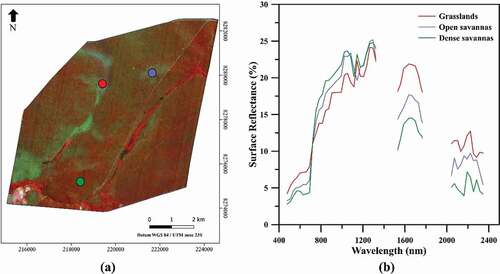
Because of the decrease in red and SWIR reflectance and the increase in NIR reflectance for areas with increasing biomass, VIs like NDVI, EVI and NDII had positive correlations with AGB. As shown in Figure 4b, the chlorophyll absorption band at 677 nm and the leaf water spectral feature at 1200 nm were most apparent in spectra of dense savanna areas.

3.2. Performance of the machine learning models and metrics to estimate AGB

The performance of the machine learning models to estimate AGB of the savannas varied with the type of metric (Figure 5a-d). However, the lowest RMSE was generally observed for RF, especially for VIs (29% in Figure 5b) and a combination of all variables (28% in Figure 5d). Thus, compared to the VIs, the corresponding model using all variables did not improve the results significantly. CART had the highest RMSE when reflectance (Figure 5a) and absorption bands (Figure 5c) were considered in the analysis and, thus, the worst predictive performance. RF differed statistically from the other models at 5% significance level when the reflectance was used as input variable, as shown by results of the post-hoc Tukey-Kramer test (Figure 5a). For VIs, RF differed from CUB, PLS and SVM (Figure 5b). Except for PLS, there were no differences between the other models for absorption bands (Figure 5c). Finally, RF was statistically different from the other models when we combined all the metrics for AGB modeling (Figure 5d).

Figure 5. Variation in the relative performance of the machine learning models to estimate aboveground biomass (AGB) of savannas when applied to the (a) reflectance of 144 Hyperion bands; (b) 22 vegetation indices (VIs); (c) 24 absorption band parameters; and (d) combination of 190 variables. The results are expressed in relative root mean square error (RMSE). For each set of metrics, upper letters indicate the statistical differences between the models (Tukey-Kramer test at 5% significance level)

The Hyperion VIs had the most stable predictive performance across models, as indicated by the small variation in RMSE values from CART to SVM (Figure 5b). By contrast, absorption band parameters (depth, width, area, and asymmetry) of the chlorophyll (680 nm), leaf water (980 nm and 1200 nm), and lignin–cellulose (1700 nm, 2100 nm, and 2300 nm) spectral features had the lowest AGB predictive performance (Figure 5c). This result was expected considering the poor SNR of Hyperion, which produced increasing noisy data from the VNIR to the SWIR, and close to the selected absorption bands. For instance, the depth of the 680-nm chlorophyll absorption increased exponentially with AGB from grasslands to dense woodland savannas (Figure 6a). On the other hand, the depth of the 1200-nm leaf water feature did not have any statistically significant relationship with AGB (Figure 6b).

Figure 6. Relationships of the aboveground biomass (AGB) with the depth of the (a) 680-nm chlorophyll and (b) 1200-nm leaf water absorption bands for grasslands, open- and dense-savanna areas

Using the RF model, the most important Hyperion reflectance bands were those positioned in the visible (681-, 671-, and 660 nm), red-edge (691- and 701 nm), NIR (884 nm) and SWIR (1568- and 2113 nm) (Figure 7a). The most important VIs in the RF model were those sensitive to canopy structure (NDVI, VARI, EVI, and VIG), biochemistry (SIPI, PSRI, PSSR, and NDII) and physiology (RENDVI) (Figure 7b). For these VIs, we observed a mean decrease in accuracy that generally ranged between 4% and 8%. The average loss in accuracy of the RF model was close to 5% for NDII and was statistically different from that of the other VIs (except VIG) at 5% significance level (Tukey-Kramer test). For the absorption bands, the top-ranked attributes were the depth and area of the 680-nm chlorophyll absorption band (Figure 7c). They were statistically different from the other absorption band parameters. When we considered all the variables in the RF model, the most important variables were the depth and area of the 680-nm absorption band, EVI, PSSR, NDVI, RENDVI, SIPI and the reflectance of the bands centered at 671 nm and 681 nm (Figure 7d).

Figure 7. The most important (a) Hyperion reflectance bands, (b) narrowband vegetation indices (VIs), (c) absorption band parameters and (d) combination of attributes captured by the Random Forest (RF) model, as expressed by values of mean decrease in accuracy. Letters indicate the statistical differences between the VIs at 5% significance level (Tukey-Kramer test)

Some VIs (e.g. NDVI and PSSR) increased with large amounts of AGB from grasslands to dense woodland savannas, while others (e.g. SIPI and PSRI) had inverse relationships with this biophysical parameter (Figure 8a-d). For most VIs, the relationships with AGB were not linear. For dense savanna areas, there was no evidence of signal saturation for the current AGB values and for VIs like NDVI (Figure 8a), PSSR (Figure 8b), PSRI (Figure 8c) and SIPI (Figure 8d).

Figure 8. Relationships of aboveground biomass (AGB) of savannas with (a) NDVI, (b) PSSR, (c) PSRI, and (d) SIPI. The relationships are statistically significant at 95% confidence level

When the cross-validation with stratified random permutations (100 repetitions) was applied to the training (80%) and validation (20%) samples, we observed underestimates of AGB with increasing vegetation cover from grasslands to dense woodland savannas (Figure 9a). The studentized residuals increased from grasslands and open savannas to dense savanna areas (Figure 9b). We detected two outliers that were removed from analysis before data reprocessing (results not shown). The relative RMSE was 26.36% for grasslands, 35.04% for open savannas and 24.85% for dense savannas (Table 3). These RMSE values were computed using the validation samples, thus not included during training of the model.

Figure 9. (a) Predicted versus observed aboveground biomass (AGB) of savannas for the validation set of samples. The out-of-samples (OOS) are plotted with the standard deviation bars. (b) Observed increase in studentized residuals with increasing AGB from grasslands to dense savanna areas

Table 3. Cross-validation assessment by savanna vegetation types. N₁ is the number of field sample plots, while N₂ is the number of validation samples from the 100 cross-validation iterations, that is, the 20% samples not used in the model training on each of the 100 iterations

Vegetation type	N1	N2	Mean AGB (Mg.ha^−1)	Standard deviation (Mg.ha^−1)	Predicted mean AGB (Mg.ha^−1)	Predicted standard deviation (Mg.ha^−1)	RMSE	%RMSE
Grasslands	11	211	4.15	0.69	4.91	0.70	1.09	26.36
Open savannas	12	216	12.56	5.29	14.72	6.32	4.40	35.04
Dense savannas	20	373	25.88	6.52	24.01	4.56	6.43	24.85

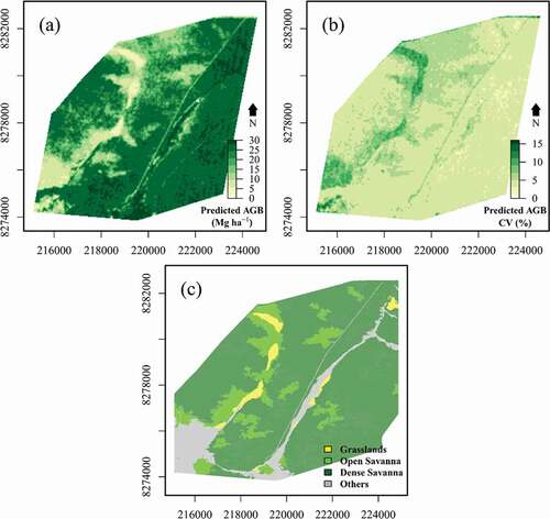
Despite these uncertainties, the AGB estimates derived from the RF and VIs showed consistent results with the vegetation cover map of the study area (Figure 10). Portions of the ESAE with AGB lower than 10 Mg.ha⁻¹ in Figure 10a were coincident with the occurrence of savanna grasslands and shrub savannas (grasslands) in Figure 10c. On the other hand, areas with AGB higher than 25 Mg.ha⁻¹ matched the woodland savanna and dense savanna woodland areas (dense savannas). The largest values of coefficient of variation (CV) were observed over grasslands and open savannas, as deduced from the comparison of Figure 10b and 10c. These values express the soil background influence on the VI determination, which causes larger spectral variability than that observed in dense vegetated areas.

Figure 10. (a) Aboveground biomass (AGB) estimates from Random Forest (RF) when applied to 22 Hyperion vegetation indices. (b) Image of the coefficient of variation (CV) showing higher values over grasslands and open savannas than over dense savannas. (c) Vegetation map of the corresponding portion of the Ecological Station of Águas Emendadas (ESAE). The map was adapted from GeoLógica/Ecotech (2009) and Jacon et al. (2017)

4. Discussion

The current investigation makes some important contributions for the AGB modeling in the savanna environment. As far as we know, this is the first hyperspectral study to estimate AGB in the Brazilian savannas. Thus, it contributes to set a baseline for estimating biomass in the Cerrado with hyperspectral data. When compared to multispectral sensors, hyperspectral instruments produce a large set of metrics for machine learning approaches, which can reduce the uncertainties in data modeling. Some of the metrics are unique in providing biophysical and biochemical information on the savannas, especially those associated with absorption bands by leaf and canopy constituents.

This study indicates which types of metrics and models produce the best predictive performance when estimating AGB for this biome, the second-largest source of carbon emissions in Brazil (De Miranda et al. 2014). This knowledge is therefore important for defining policies to reduce emissions and mitigate environmental climate changes. By using Hyperion data, our study also anticipates the potential of hyperspectral metrics and machine learning models to estimate AGB, considering the future transition from sampling-type hyperspectral missions (< 10 km of swath) to large-coverage hyperspectral satellites (> 100 km of swath). Our results over the ESAE showed decreasing relative RMSE from grasslands to dense savanna areas up to values of 28% (combination of metrics). This result is acceptable if we consider the delay of one year between the fieldwork activities and the Hyperion image acquisition as well as the relationships between rainfall seasonality and vegetation phenology. However, this value is still higher than the requirements of the SAR-based BIOMASS mission planned for 2022 (20% RMSE) (Le Toan et al. 2011; Bispo et al. 2020). To achieve this requirement in our work, it will be probably necessary to combine hyperspectral data with observations from other technologies.

Imaging spectrometers can complement the information provided by SAR and LiDAR, which are technologies that capture more efficiently the attributes of canopy structure. SAR and LiDAR are especially important to estimate AGB over dense vegetated areas. For instance, when combining airborne LiDAR and hyperspectral data over the Amazonian tropical forests, Almeida et al. (2019) observed an improvement in accuracy of the AGB estimates of 15% for RMSE when compared to single LiDAR models. In a recent study over the savannas in Brazil, Bispo et al. (2020) combined Operational Land Imager (OLI)/Landsat-8 data and SAR observations from Phased Array L-band Synthetic Aperture Radar (PALSAR-2) to estimate AGB using a RF model. They observed high uncertainties when estimating AGB over grassland areas, which was consistent with our results at the ESAE.

Currently, there are not large swath-width hyperspectral missions to allow such combination over the entire savanna biome in Brazil. However, the recently launched PRecursore IperSpettrale della Missione Applicativa (PRISMA) can be useful for this purpose at least locally. PRISMA has a swath width of 30 km and a SNR higher than 200:1 in the visible and NIR interval. In the SWIR, the nominal SNR is almost three times better than Hyperion. PRISMA acquires images in 234 bands in the 400–2500 nm range with spatial resolution of 30 m and a revisit time of approximately one month (Niroumand-Jadidi, Bovolo, and Bruzzone 2020). Therefore, PRISMA data can be combined with SAR or LiDAR observations for AGB modeling at larger areas than those observed by Hyperion. PRISMA has also a panchromatic camera with 5 m spatial resolution. At this level of spatial resolution, texture metrics can be considered as potential predictors of AGB, as demonstrated in other studies (Ploton et al. 2017). As a result, PRISMA will probably increase the number of predictors for the models and improve the AGB estimates compared to Hyperion in future studies. This is important for supporting REDD+ projects and carbon markets.

From the tested machine learning models, our findings showed that RF, presenting the lowest RMSE, was the most promising approach to estimate AGB of the savannas using a great number of hyperspectral metrics. Some degree of overfitting may exist in the results because we did not apply any feature selection procedure over the data. However, this effect is probably small. For instance, the RMSE obtained for RF was lower for 22 VIs than for 144 reflectance bands. Moreover, by testing a correlation feature selection method (findCorrelation function from the caret R package; threshold of 0.90), we observed just a small increase in the RMSE from 28% to 29% after the reduction in the number of variables from 22 to 15 VIs. Therefore, our approach offered the same set of metrics for all models. Some of them (e.g. PLS) assume the existence a priori of correlated data or may work well with correlated features (e.g. SVM).

The best performance of the RF (low RMSE) can be attributed to its ability to deal with the nonlinearity present in the data such as that observed in the relationships between AGB and VIs. However, the performance of the models varied with the type of metric. Almeida et al. (2019) had a similar result for tropical forests. In hyperspectral classification studies, the overall accuracy of RF using VIs has been also superior to the accuracy obtained from other classifiers for discriminating savanna physiognomies (Toniol et al. 2017).

In our study, the most important Hyperion bands in the RF model were positioned in the visible, red-edge and NIR. This result confirms the importance of the VNIR spectral interval in the studies of savannas in Brazil (Toniol et al. 2017). Consequently, the top-ranked VIs in the RF model included NIR-visible (NDVI, SIPI, PSRI, and EVI), visible-visible (VARI and VIG), NIR-red edge (PSRI and RENDVI), and NIR-SWIR (NDII) pairs of bands in their formulations. This large range of spectral coverage of VI operation captured the information of different savanna properties associated with canopy structure, biochemistry, and plant physiology (Roberts, Roth, and Perroy 2012). These VIs also captured the increasing influence of the soil surface (soil plus non-photosynthetic vegetation) over the sensor signal from dense woodland savannas to open savannas. Because of the well-defined vegetation gradient observed in the study area, these VIs were correlated with the AGB in positive or negative associations. For instance, the transition from grasslands (low AGB) to dense savanna areas (high AGB) produces lower reflectance in the visible (chlorophyll absorption), higher reflectance in the NIR (canopy scattering), and lower reflectance in the SWIR (canopy moisture). This fact was well illustrated in our work by the Hyperion reflectance spectra. Consequently, VIs like NDVI and NDII were positively correlated with AGB, while others (e.g. SIPI and PSRI) showed inverse relationships with this biophysical attribute. Most of them showed non-linear relationships with the AGB.

Our results showed that the depth and area of the 680-nm absorption band were the most important metrics to estimate AGB among the band parameters. Contrary to reports for tropical forests (Almeida et al. 2019), the leaf-water absorption bands (980 nm and 1200 nm) were not correlated with the AGB in our study. Leaf water features are also sensitive to changes in leaf area index (LAI) and are generally correlated with AGB (Roberts, Roth, and Perroy 2012). Our results did not confirm this pattern with Hyperion data probably due to noise. Using Hyperion data, the poor instrumental SNR at these wavelengths added significant noise into the analysis, creating difficulties to observe the possible existence of such relationships. Consequently, absorption band parameters were the worst hyperspectral metrics captured by the RF model to estimate AGB.

Our data modeling refers to the dry season. In the savanna environment, the physiognomies have different sensitivities to rainfall seasonality. For instance, grasslands are more sensitive to water deficit in the dry season than woodlands because the herbaceous plants and grasses generally have shallow roots to access soil water (Felfili et al. 2008; Jacon et al. 2017). On the other hand, grasslands present higher rates of green-up than woodlands after the first rainfall events, which produce significant changes in the seasonal response of the VIs. In a study by Jacon et al. (2017), the largest rates of changes between the rainy and dry seasons of the ESAE were observed for VARI, VIG, and NDII over the savanna grasslands and shrub savannas. In the present work, these three VIs have been selected by the Hyperion RF model as important variables to estimate AGB.

Finally, it is important to recognize the uncertainties in the data analysis of the current work and the possible error propagation from field AGB estimates using allometry to satellite AGB prediction using hyperspectral metrics. For instance, the model proposed by Rezende et al. (2006) to determine the AGB of the plots had a sampling error of 25.79%. Our hyperspectral AGB estimates had RMSE close to 29%. In addition, the stratified sampling approach that we employed for creating training and validation datasets likely affected the performance of the models due to the relatively small number of samples used in the data analysis (n = 45 sample plots). Other sources of uncertainties described by Baraloto et al. (2012) in forest inventories include plot size and plot shape. When using remote sensing data, plot location over the images and the temporal delay between field and satellite observations cause errors in the AGB estimates. In spite of these uncertainties, the mean AGB values reported in this study over the savanna physiognomies were generally consistent with the values published by different researchers in other Cerrado areas (e.g. Kauffman, Cummings, and Ward 1994; Ribeiro et al. 2011).

5. Conclusions

The results indicated the most important hyperspectral metrics and machine learning models to predict the AGB of savannas in Brazil. For most metrics, the lowest RMSE was observed for RF. The Hyperion VIs presented the most stable predictive performance across the models. The top ranked indices in the RF model were the NDVI, PSSR, EVI, RENDVI, SIPI, PSRI, VARI, VIG, and NDII. The resultant AGB map from RF and VIs was consistent with an available vegetation cover map of the ESAE. Areas with AGB lower than 10 Mg.ha⁻¹ coincided with grassland physiognomies (savanna grasslands and shrub savannas). On the other hand, areas with AGB higher than 25 Mg.ha⁻¹ matched the occurrence of dense savanna physiognomies (woodland savanna and dense savanna woodland). The RMSE of the RF model with VIs was 29%, decreasing to 28% when all the variables were used in the analysis. The CV was higher over the grasslands than over the dense savannas.

Our study contributes to establish a starting point of models and metrics over the savannas for the future transition from sampling-type hyperspectral missions (< 10 km of swath) to large-coverage hyperspectral satellites (> 100 km of swath). The predictive performance of the metrics to estimate AGB will probably improve, considering the recent technological advances in SNR of the imaging spectrometers.

Acknowledgements

The authors are grateful to the Instituto Brasília Ambiental (IBRAM) for the research authorization 06/2015 (project number 391.000.740/2015). We also thank field assistance provided by the Empresa Brasileira de Pesquisa Agropecuária (Embrapa – Cerrados), especially by José Ferreira Paixão. Lênio S. Galvão was supported by the Conselho Nacional de Desenvolvimento Científico e Tecnológico (CNPq) (grant number 301486/2017-4), while Ricardo Dalagnol was supported by the Fundação de Amparo à Pesquisa do Estado de São Paulo (FAPESP) (grant number 2019/21662-8). The authors thanks the anonymous reviewers for the nice comments and suggestions.

Disclosure statement

The data that support the main conclusions of this study are available at https://figshare.com/s/e12fb88de75eac0e6f6b.

Additional information

Funding

This work was supported by the Conselho Nacional de Desenvolvimento Científico e Tecnológico [301486/2017-4]; Fundação de Amparo à Pesquisa do Estado de São Paulo [2019/21662-8].

References

- Almeida, C. T., L. S. Galvão, L. E. O. C. Aragão, J. P. H. B. Ometto, A. D. Jacon, F. R. D. S. Pereira, L. Y. Sato, et al. 2019. “Combining LiDAR and Hyperspectral Data for Aboveground Biomass Modeling in the Brazilian Amazon Using Different Regression Algorithms.” Remote Sensing of Environment 232 :111323. doi:https://doi.org/10.1016/j.rse.2019.111323.
- Baraloto, C., Q. Molto, S. Rabaud, B. Herault, R. Valencia, L. Blanc, P. V. A. Fine, and J. Thompson. 2012. “Rapid Simultaneous Estimation of Aboveground Biomass and Tree Diversity across Neotropical Forests: A Comparison of Field Inventory Methods.” Biotropica 45 (3): 288–298. doi:https://doi.org/10.1111/btp.12006.
- Basak, D., S. Pal, and D. C. Patranabis. 2017. “Support Vector Regression.” Neural Information Processing Letters and Reviews 11: 203–224. doi:https://doi.org/10.1007/978-3-319-70087-8_72.
- Bispo, P. D. C., P. Rodríguez-Veiga, B. Zimbres, S. C. Miranda, C. H. G. Cezare, S. Fleming, F. Baldacchino, et al. 2020. “Woody Aboveground Biomass Mapping of the Brazilian Savanna with a Multi-Sensor and Machine Learning Approach.” Remote Sensing 12 (17): 2685. doi:https://doi.org/10.3390/rs12172685.
- Bitencourt, M. D., J. H. N. de Mesquita, G. Kuntschik, H. R. Da Rocha, and P. Furley. 2007. “Cerrado Vegetation Study Using Optical and Radar Remote Sensing: Two Brazilian Case Studies.” Canadian Journal of Remote Sensing 33 (6): 468–480. doi:https://doi.org/10.5589/m07-054.
- Blackburn, G. A. 1998. “Spectral Indices for Estimating Photosynthetic Pigment Concentrations: A Test Using Senescent Tree Leaves.” International Journal of Remote Sensing 19 (4): 657–675. doi:https://doi.org/10.1080/014311698215919.
- Braun, A., J. Wagner, and V. Hochschild. 2018. “Above-ground Biomass Estimates Based on Active and Passive Microwave Sensor Imagery in Low-biomass Savanna Ecosystems.” Journal of Applied Remote Sensing 12 (4): 046027. doi:https://doi.org/10.1117/1.JRS.12.046027.
- Breiman, L. E. O. 2001. “Random Forest.” Machine Learning 45 (1): 5–32. doi:https://doi.org/10.1023/A:1010933404324.
- Daughtry, C. S. T. 2001. “Agroclimatology: Discriminating Crop Residues from Soil by Shortwave Infrared Reflectance.” Agronomy Journal 93 (1): 125–131. doi:https://doi.org/10.2134/agronj2001.931125x.
- Daughtry, C. S. T., C. L. Walthall, M. S. Kim, E. Brown De Colstoun, and J. E. McMurtrey III. 2000. “Estimating Corn Leaf Chlorophyll Concentration from Leaf and Canopy Reflectance.” Remote Sensing of Environment 74 (2): 229–239. doi:https://doi.org/10.1016/S0034-4257(00)00113-9.
- De Miranda, S. D. C., M. M. C. Bustamante, M. Palace, S. Hagen, M. Keller, and L. G. Ferreira. 2014. “Regional Variations in Biomass Distribution in Brazilian Savanna Woodland.” Biotropica 46 (2): 125–138. doi:https://doi.org/10.1111/btp.12095.
- De Oliveira, L. M., L. S. Galvão, and F. J. Ponzoni. 2019. “Topographic Effects on the Determination of Hyperspectral Vegetation Indices: A Case Study in Southeastern Brazil.” Geocarto International 1–18. doi:https://doi.org/10.1080/10106049.2019.1690055.
- Felfili, J. M., F. A. Carvalho, and R. F. Haidar. 2005. Manual para o monitoramento de parcelas permanentes nos biomas Cerrado e Pantanal (ISBN 85–87599). Brasília: EdUnB. 55
- Felfili, J. M., M. C. Silva Jr, R. C. Mendonça, C. W. Fagg, T. S. Filgueiras, and V. V. Mecenas. 2008. “Vegetação E Flora: Fitofisionomias E Flora.” In Águas Emendadas /Distrito Federal, edited by F. O. Fonseca, 152–155. Brasília: Secretaria de Estado de Desenvolvimento Urbano e Meio Ambiente - SEDUMA.
- Ferreira, L. G., G. P. Asner, D. E. Knapp, E. A. Davidson, M. Coe, M. M. C. Bustamante, and E. L. Oliveira. 2011. “Equivalent Water Thickness in Savanna Ecosystems: MODIS Estimates Based on Ground and EO-1 Hyperion Data.” International Journal of Remote Sensing 32 (22): 7423–7440. doi:https://doi.org/10.1080/01431161.2010.523731.
- Forkuor, G., J. B. Zoungrana, K. Dimobe, B. Ouattara, K. P. Vadrevu, and J. E. Tondoh. 2020. “Above-ground Biomass Mapping in West African Dryland Forest Using Sentinel-1 and 2 Datasets - A Case Study.” Remote Sensing of Environment 236: 111496. doi:https://doi.org/10.1016/j.rse.2019.111496.
- Friedman, J. H. 2002. “Stochastic Gradient Boosting.” Computational Statistics & Data Analysis 38 (4): 367–378. doi:https://doi.org/10.1016/S0167-9473(01)00065-2.
- Galvão, L. S., A. R. Formaggio, and D. A. Tisot. 2005. “Discrimination of Sugarcane Varieties in Southeastern Brazil with EO-1 Hyperion Data.” Remote Sensing of Environment 94 (4): 523–534. doi:https://doi.org/10.1016/j.rse.2004.11.012.
- Galvão, L. S., A. A. Souza, and F. M. Breunig. 2019. “A Hyperspectral Experiment over Tropical Forests Based on the EO-1 Orbit Change and PROSAIL Simulation.” GIScience & Remote Sensing 57 (1): 74–90. doi:https://doi.org/10.1080/15481603.2019.1668595.
- Gamon, J. A., L. Serrano, and J. S. Surfus. 1997. “The Photochemical Reflectance Index: An Optical Indicator of Photosynthetic Radiation-Use Efficiency across Species, Functional Types, and Nutrient Levels.” Oecologia 112 (4): 492–501. doi:https://doi.org/10.1007/s004420050337.
- Gao, B. 1996. “A Normalized Difference Water Index for Remote Sensing of Vegetation Liquid Water from Space.” Remote Sensing of Environment 58 (3): 257–266. doi:https://doi.org/10.1016/S0034-4257(96)00067-3.
- GeoLógica/Ecotech. 2009. “Plano De Manejo: Programa De Proteção, Planejamento E Gestão Para a Estação Ecológica De Águas Emendadas (ESEC-AE).” Brasília: Instituto Brasília Ambiental, IBRAM.
- Gitelson, A. A., Y. J. Kaufman, R. Stark, and D. Rundquist. 2002b. “Novel Algorithms for Remote Estimation of Vegetation Fraction.” Remote Sensing of Environment 80 (1): 76–87. doi:https://doi.org/10.1016/S0034-4257(01)00289-9.
- Gitelson, A. A., M. N. Merzlyak, and O. B. Chivkunova. 2001. “Optical Properties and Nondestructive Estimation of Anthocyanin Content in Plant Leaves.” Photochemistry and Photobiology 74 (1): 38–45. doi:https://doi.org/10.1562/0031-8655(2001)074<0038:OPANEO>2.0.CO;2.
- Gitelson, A. A., M. N. Merzlyak, and H. K. Lichtenthaler. 1996. “Detection of Red Edge Position and Chlorophyll Content by Reflectance Measurements near 700 Nm.” Journal of Plant Physiology 148 (3–4): 501–508. doi:https://doi.org/10.1016/S0176-1617(96)80285-9.
- Gitelson, A. A., Y. Zur, O. B. Chivkunova, and M. N. Merzlyak. 2002a. “Assessing Carotenoid Content in Plant Leaves with Reflectance Spectroscopy.” Photochemistry and Photobiology 75 (3): 272–281. doi:https://doi.org/10.1562/0031-8655(2002)075<0272:accipl>2.0.CO;2.
- Goodenough, D. G., A. Dyk, O. Niemann, J. S. Pearlman, H. Chen, T. Han, M. Murdoch, and C. West. 2003. “Processing Hyperion and ALI for Forest Classification.” IEEE Transactions on Geoscience and Remote Sensing 41 (6): 1321–1331. doi:https://doi.org/10.1109/TGRS.2003.813214.
- Grace, J., J. S. José., P. Meir, H. S. Miranda, and R. A. Montes. 2016. “Productivity and Carbon Fluxes of Tropical Savannas.” Journal of Biogeography 33 (3): 387–400. doi:https://doi.org/10.1111/j.1365-2699.2005.01448.x.
- Horler, D. N. H., M. Dockray, and J. Barber. 1983. “The Red-Edge of Plant Leaf Reflectance.” International Journal of Remote Sensing 4 (2): 273–288. doi:https://doi.org/10.1080/01431168308948546.
- Houghton, R. A., F. Hall, and S. J. Goetz. 2009. “Importance of Biomass in the Global Carbon Cycle.” Journal of Geophysical Research 114 (G2): 1–13. doi:https://doi.org/10.1029/2009JG000935.
- Huete, A. R., K. Didan, T. Miura, E. P. Rodriguez, X. Gao, and L. G. Ferreira. 2002. “Overview of the Radiometric and Biophysical Performance of the MODIS Vegetation Indices.” Remote Sensing of Environment 83 (1–2): 195–213. doi:https://doi.org/10.1016/S0034-4257(02)00096-2.
- Hunt, E. R., and B. N. Rock. 1989. “Detection of Changes in Leaf-Water Content Using near Infrared and Middle-Infrared Reflectances.” Remote Sensing of Environment 30: 43–54.
- Jacon, A. D., L. S. Galvão, J. R. Dos Santos, and E. E. Sano. 2017. “Seasonal Characterization and Discrimination of Savannah Physiognomies in Brazil Using Hyperspectral Metrics from Hyperion/EO-1.” International Journal of Remote Sensing 38 (15): 4494–4516. doi:https://doi.org/10.1080/01431161.2017.1320443.
- Kauffman, J. B., D. L. Cummings, and D. E. Ward. 1994. “Relationships of Fire, Biomass and Nutrient Dynamics along a Vegetation Gradient in the Brazilian Cerrado.” The Journal of Ecology 82 (3): 519–531. doi:https://doi.org/10.2307/2261261.
- Kaufman, Y. J., D. Tanré, L. A. Remer, E. F. Vermote, A. Chu, and B. N. Holben. 1997. “Operational Remote Sensing of Tropospheric Aerosol over Land from EOS Moderate Resolution Imaging Spectroradiometer.” Journal of Geophysical Research 102 (D14): 17051–17067. doi:https://doi.org/10.1029/96JD03988.
- Kokaly, R. F., and A. K. Skidmore. 2015. “Plant Phenolics and Absorption Features in Vegetation Reflectance Spectra near 1.66 µm.” International Journal of Applied Earth Observations and Geoinformation 43: 55–83. doi:https://doi.org/10.1016/j.jag.2015.01.010.
- Kuhn, M. 2008. “Building Predictive Models in R Using the Caret Package.” Journal of Statistical Software 28 (5): 1–26. doi:https://doi.org/10.18637/jss.v028.i05.
- Le Toan, T., S. Quegan, M. Davidson, H. Balzter, P. Paillou, K. Papathanassiou, S. Plummer, et al. 2011. “The BIOMASS Mission: Mapping Global Forest BIOMASS to Better Understand the Terrestrial Carbon Cycle.” Remote Sensing of Environment 115 (11): 2850–2860. doi:https://doi.org/10.1016/j.rse.2011.03.020.
- Liesenberg, V., L. S. Galvão, and F. J. Ponzoni. 2007. “Variations in Reflectance with Seasonality and Viewing Geometry: Implications for Classification of Brazilian Savanna Physiognomies with MISR/Terra Data.” Remote Sensing of Environment 107 (1–2): 276–286. doi:https://doi.org/10.1016/j.rse.2006.03.018.
- Merton, R., and J. Huntington. 1999. “Early Simulation of the ARIES-1 Satellite Sensor for MultiTemporal Vegetation Research Derived from AVIRIS.” Paper Presented at the JPL Airborne Earth Science Workshop 8, Pasadena, USA, February 9–11, pp. 299–307.
- Merzlyak, M. N., A. A. Gitelson, O. B. Chivkunova, and V. Y. U. Rakitin. 1999. “Non-Destructive Optical Detection of Pigment Changes during Leaf Senescence and Fruit Ripening.” Physiologia Plantarum 106 (1): 135–141. doi:https://doi.org/10.1034/j.1399-3054.1999.106119.x.
- Miguel, E. P., A. V. Rezende, F. A. Leal, E. A. T. Matricardi, A. T. D. Vale, and R. S. Pereira. 2015. “Redes Neurais Artificiais Para a Modelagem Do Volume De Madeira E Biomassa Do Cerradão Com Dados De Satélite.” Pesquisa Agropecuária Brasileira 50 (9): 829–839. doi:https://doi.org/10.1590/S0100-204X2015000900012.
- Muumbe, T. P., J. Baade, J. Singh, C. Schmullius, and C. Thau. 2021. “Terrestrial Laser Scanning for Vegetation Analyses with a Special Focus on Savannas.” Remote Sensing 13 (3): 507. doi:https://doi.org/10.3390/rs13030507.
- Myers, N., R. A. Mittermeier, C. G. Mittermeier, G. A. B. Fonseca, and J. Kent. 2000. “Biodiversity Hotspots for Conservation Priorities.” Nature 403 (6772): 853–858. doi:https://doi.org/10.1038/35002501.
- Niroumand-Jadidi, M., F. Bovolo, and L. Bruzzone. 2020. “Water Quality Retrieval from PRISMA Hyperspectral Images: First Experience in a Turbid Lake and Comparison with Sentinel-2.” Remote Sensing 12 (23): 3984. doi:https://doi.org/10.3390/rs12233984.
- Nunes, M. H., E. B. Gorgens, and A. R. Hernandez Montoya. 2016. “Artificial Intelligence Procedures for Tree Taper Estimation within a Complex Vegetation Mosaic in Brazil.” PLoS One 11 (5): e0154738. doi:https://doi.org/10.1371/journal.pone.0154738.
- Oliveira-Filho, A. T., and J. A. Ratter. 2002. “Vegetation Physiognomies and Woody Flora of the Cerrado Biome.” In The Cerrados of Brazil, edited by P. S. Oliveira and R. J. Marquis, 91–120. New York: Columbia University Press.
- Pearlman, J. S., P. S. Barry, C. C. Segal, J. Shepanski, D. Beiso, and S. L. Carman. 2003. “Hyperion, a Space-based Imaging Spectrometer.” IEEE Transactions on Geoscience and Remote Sensing 41 (6): 1160–1173. doi:https://doi.org/10.1109/TGRS.2003.815018.
- Peñuelas, J., F. Baret, and I. Filella. 1995. “Semiempirical Indexes to Assess Carotenoids Chlorophyll-A Ratio from Leaf Spectral Reflectance.” Photosynthetica 31: 221–230.
- Peñuelas, J., J. Pinol, R. Ogaya, and I. Lilella. 1997. “Estimation of Plant Water Content by the Reflectance Water Index WI (R900/R970).” International Journal of Remote Sensing 18 (13): 2869–2875. doi:https://doi.org/10.1080/014311697217396.
- Ploton, P., N. Barbier, P. Couteron, C. M. Antin, N. Ayyappan, N. Balachandran, and N. Barathan. 2017. “Toward a General Tropical Forest Biomass Prediction Model from Very High Resolution Optical Satellite Images.” Remote Sensing of Environment 200: 140–153. doi:https://doi.org/10.1016/j.rse.2017.08.001.
- R Development Core Team. 2021. “R: A Language and Environment for Statistical Computing.” In R Foundation for Statistical Computing, Vienna, Austria. https://www.R-project.org/
- Rasanen, A., S. Juutinen, M. Kalacska, M. Aurela, P. Heikkinen, K. Maenpaa, A. Rimali, and T. Virtanen. 2020. “Peatland Leaf-area Index and Biomass Estimation with Ultra-high Resolution Remote Sensing.” GIScience & Remote Sensing 57 (7): 943–964. doi:https://doi.org/10.1080/15481603.2020.1829377.
- Ratter, J. A., S. Bridgewater, and J. F. Ribeiro. 2006. “Biodiversity Patterns of the Woody Vegetation of the Brazilian Cerrados.” In Neotropical Savannas and Seasonally Dry Forests, edited by T. Penington and J. A. Ratter, 31–66. London: Taylor & Francis.
- Rezende, A. V., A. T. Do Vale, C. R. Sanquetta, A. Figueiredo Filho, and J. M. Felfili. 2006. “Comparação De, Modelos Matemáticos Para Estimativa Do Volume, Biomassa E Estoque De Carbono Da Lenhosa De Um Cerrado Sensu Stricto Em Brasília DF.” Scientia Forestalis 71: 65–76.
- Ribeiro, J. F., and B. M. T. Walter. 1998. “Fitofisionomias do Bioma Cerrado.” In Cerrado: Ambiente e Flora, edited by S. M. Sano and S. P. Almeida, 87–166. Planaltina: EMBRAPA-CPAC.
- Ribeiro, S. C., L. Fehrmann, C. P. B. Soares, L. A. G. Jacovine, C. Kleinn, and R. O. Gaspar. 2011. “Above- and Belowground Biomass in a Brazilian Cerrado.” Forest Ecology and Management 262 (3): 491–499. doi:https://doi.org/10.1016/j.foreco.2011.04.017.
- Roberts, D. A., K. L. Roth, and R. L. Perroy. 2012. “Hyperspectral Vegetation Indices.” In Hyperspectral Remote Sensing of Vegetation, edited by P. S. Thenkabail, J. G. Lyon, and A. Huete, 309–327. Boca Raton, FL: CRC Press, Taylor and Francis Group.
- Rouse, J. W., R. H. Haas, J. A. Schell, and D. W. Deering. 1973. “Monitoring Vegetation Systems in the Great Plains with ERTS.” Paper Presented at the Third ERTS-1 Symposium, Washington, DC: NASA SP-351, December 10–14, Vol. 1. pp. 309–317.
- Sanches, I. D. A., C. R. Souza Filho, and R. F. Kokaly. 2014. “Spectroscopic Remote Sensing of Plant Stress at Leaf and Canopy Levels Using the Chlorophyll 680nm Absorption Feature with Continuum Removal.” ISPRS Journal of Photogrammetry and Remote Sensing 97: 111–122. doi:https://doi.org/10.1016/j.isprsjprs.2014.08.015.
- Sankaran, M., N. Hanan, R. Scholes, J. Ratnam, D. J. Augustine, B. S. Cade, J. Gignoux, et al. 2005. “Determinants of Woody Cover in African Savannas.” Nature 438 (7069): 846–849. doi:https://doi.org/10.1038/nature04070.
- Sano, E. E., L. G. Ferreira, and A. R. Huete. 2005. “Synthetic Aperture Radar (L-band) and Optical Vegetation Indices for Discriminating the Brazilian Savanna Physiognomies: A Comparative Analysis.” Earth Interactions Paper 9: 15.
- Sano, E. E., R. Rosa, J. L. S. Brito, and L. G. Ferreira. 2010. “Land Cover Mapping of the Tropical Savanna Region in Brazil.” Environmental Monitoring and Assessment 166 (1–4): 113–124. doi:https://doi.org/10.1007/s10661-009-0988-4.
- Schwieder, M., P. J. Leitão, J. R. R. Pinto, A. M. C. Teixeira, F. Pedroni, M. Sanchez, M. M. Bustamante, and P. Hostert. 2018. “Landsat Phenological Metrics and Their Relation to Aboveground Carbon in the Brazilian Savanna.” Carbon Balance and Management 13 (1): 7. doi:https://doi.org/10.1186/s13021-018-0097-1.
- Serrano, L., J. Peñuelas, and S. L. Ustin. 2002. “Remote Sensing of Nitrogen and Lignin in Mediterranean Vegetation from AVIRIS Data: Decomposing Biochemical from Structural Signals.” Remote Sensing of Environment 81 (2–3): 355–364. doi:https://doi.org/10.1016/S0034-4257(02)00011-1.
- Sibanda, M., O. Mutanga, and M. Rouget. 2016. “Comparing the Spectral Settings of the New Generation Broad and Narrow Band Sensors in Estimating Biomass of Native Grasses Grown under Different Management Practices.” GIScience & Remote Sensing 53 (5): 614–633. doi:https://doi.org/10.1080/15481603.2016.1221576.
- Souza, A. A. D., L. S. Galvão, T. S. Korting, and J. D. Prieto. 2020. “Dynamics of Savanna Clearing and Land Degradation in the Newest Agricultural Frontier in Brazil.” GIScience & Remote Sensing 57 (7): 965–984. doi:https://doi.org/10.1080/15481603.2020.1835080.
- Toniol, A. C., L. S. Galvão, F. J. Ponzoni, E. E. Sano, and D. J. Amore. 2017. “Potential of Hyperspectral Metrics and Classifiers for Mapping Brazilian Savannas in the Rainy and Dry Seasons.” Remote Sensing Applications: Society and Environment 8: 20–29. doi:https://doi.org/10.1016/j.rsase.2017.07.004.
- Vogelmann, J. E., B. N. Rock, and D. M. Moss. 1993. “Red Edge Spectral Measurements from Sugar Maple Leaves.” International Journal of Remote Sensing 14: 1563–1575. doi:https://doi.org/10.1080/01431169308953986.
- Wessels, K., R. Mathieu, N. Knox, R. Main, L. Naidoo, and K. Steenkamp. 2019. “Mapping and Monitoring Fractional Woody Vegetation Cover in the Arid Savannas of Namibia Using LiDAR Training Data, Machine Learning, and ALOS PALSAR Data.” Remote Sensing 11 (22): 2633. doi:https://doi.org/10.3390/rs11222633.
- Zalles, V., M. C. Hansen, P. V. Potapov, S. V. Stehman, A. Tyukavina, A. Pickens, X. P. Song, et al. 2019. “Near Doubling of Brazil’s Intensive Row Crop Area since 2000.” Proceedings of the National Academy of Sciences of the United States of America 116 (2): 428–435. doi:https://doi.org/10.1073/pnas.1810301115.