RoadVecNet: a new approach for simultaneous road network segmentation and vectorization from aerial and google earth imagery in a complex urban set-up

ABSTRACT

In this study, we present a new automatic deep learning-based network named Road Vectorization Network (RoadVecNet), which comprises interlinked UNet networks to simultaneously perform road segmentation and road vectorization. Particularly, RoadVecNet contains two UNet networks. The first network with powerful representation capability can obtain more coherent and satisfactory road segmentation maps even under a complex urban set-up. The second network is linked to the first network to vectorize road networks by utilizing all of the previously generated feature maps. We utilize a loss function called focal loss weighted by median frequency balancing (MFB_FL) to focus on the hard samples, fix the training data imbalance problem, and improve the road extraction and vectorization performance. A new module named dense dilated spatial pyramid pooling, which combines the benefit of cascaded modules with atrous convolution and atrous spatial pyramid pooling, is designed to produce more scale features over a broader range. Two types of high-resolution remote sensing datasets, namely, aerial and Google Earth imagery, were used for road segmentation and road vectorization tasks. Classification results indicate that the RoadVecNet outperforms the state-of-the-art deep learning-based networks with 92.51% and 93.40% F1 score for road surface segmentation and 89.24% and 92.41% F1 score for road vectorization from the aerial and Google Earth road datasets, respectively. In addition, the proposed method outperforms the other comparative methods in terms of qualitative results and produces high-resolution road segmentation and vectorization maps. As a conclusion, the presented method demonstrates that considering topological quality may result in improvement of the final road network, which is essential in various applications, such as GIS database updating.

GRAPHICAL ABSTRACT

KEYWORDS:

• Deep learning
• RoadVecNet
• remote sensing
• road segmentation
• GIS
• road vectorization

1. Introduction

Automatic extraction of road networks from high-resolution remote sensing imagery (HRSI) has been an active research topic in the remote sensing field (Zhang et al. 2018). The urban road network is one of the major components of a city that plays a significant role in its development and expansion. Non-spatial attributes can be integrated into the spatial information with the aid of vectorized roads, and they can then be used to efficiently model the traffic information and assist traffic management (Hong et al. 2018). However, urban road traffic networks and digital maps are incredibly tedious and time-consuming to produce and update via manual digitization of HRSI because the task has long production cycles and involves large workloads. Thus, up-to-date traffic maps are difficult to maintain (Hong et al. 2018). Automatically extracting roads from HRSI and obtaining road information with the aid of advanced image processing techniques, artificial intelligence, and machine learning tools is an efficient and economical approach. The road information can be utilized in various Geospatial Information System applications, such as vehicle navigation (Luo et al. 2019), vector map database updating (Hong et al. 2018), citizen tourism planning, and image registration (Abdollahi and Pradhan 2021). However, an accurate road extraction from the HRSI is always a challenging task. This difficulty is because of the existence of complicated features in the HRSI, such as trees, building roofs, shadows, cars, road marking lines, which result in low geometric precision when extracting road information outcomes (Gao et al. 2018). The HRSI has a large number of mixed pixels, obscuring the borders between other objects and roads. Accordingly, incorrect boundary information can be easily produced by urban roads with rich spectral information in the image data (Hormese and Saravanan 2016). Several recent works have been suggested in the literature to address these challenging issues on road extraction (Kaur and Singh 2015); however, they are far from ideal.

Traditional studies on this topic are divided into three categories: knowledge, object, and feature levels (Hong et al. 2018).

1) The knowledge level group includes road characteristics (Movaghati, Moghaddamjoo, and Tavakoli 2010) and multi-source data fusion (Qiaoping and Couloigner 2004). Road characteristic theories rely on their own features, such as context and spectral characteristics, for road extraction. The multi-source data fusion approach uses the existing road databases, such as vector maps, to assist the extraction of roads. The efficiency of such methods is not ideal, and they have complex designs.

2) The object-level group consists of regional statistics (Yi et al. 2010) and multi-resolution analysis (Shen, Luo, and Gao 2010). In the regional statistics approach, the image is initially segmented into objects, and a “word-theme” method is then built to extract roads. The multi-resolution analytical approach combines a single image at various scales or resolutions of remote sensing imagery. The initial segmentation of images by the region-based models leads to the “adhesion” phenomenon (Maboudi et al. 2017).

3) The feature level group contains the edge and parallel lines (Unsalan and Sirmacek 2012), the filter approach (Chaudhuri, Kushwaha, and Samal 2012), and template matching (Miao et al. 2012). The filter approach utilizes a special filter to enhance road pixels and extract road. However, this approach achieves low extraction accuracy in the complex areas and leads to the “salt and pepper” phenomenon. The edge and parallel lines utilize the fact that road borders are generally parallel lines. In Unsalan and Sirmacek (2012), the initial road edge was extracted, and graph theory and Binary Ballon (BB) method were used to extract roads. The template matching approach utilizes a specific template or seed pixels to form roads initially and then extract them.

Recently, deep learning models have been widely utilized in the remote sensing field, such as object detection (Ševo and Avramović 2016), image retrieval (Zhou et al. 2017), and image classification (Zhong et al. 2017). Then, these models have been adopted for extracting roads from HRSI by embedding many multi-level and high-level information to reduce false predictions, unlike the traditional methods that only utilize low-level information for road extraction (Abdollahi, Pradhan et al. 2020). Mnih and Hinton (2010) applied a deep belief network for road extraction from airborne imagery. Sarhan, Khalifa, and Nabil (2011) proposed a convolutional neural network (CNN), which takes full advantage of the geometric and spectral road characteristics, and achieved an overall accuracy (OA) of 92.50% for road extraction from the IKONOS satellite imagery. Saito and Aoki (2015) presented a CNN model and achieved 88.66% accuracy for road extraction from Massachusetts aerial imagery. Zhao, Du, and Emery (2017) introduced an object-based deep learning model with 89.59% OA for extracting road from Worldview-2 imagery. Li et al. (2016) applied a CNN model to extract roads from Pleiades-1A and GeoEye images; then they used a post-processing step to smoothen the results and obtain the road centerline and achieved 80.59% accuracy. Although certain outcomes have been achieved in road extraction by using CNN, many errors still persist. For instance, the proposed approaches were not efficient in accurately detecting roads in complex areas, and the extracted roads still have imperfect fragments and patches (Xie et al. 2019, Zhao, Shi et al. 2017; Sarhan, Khalifa, and Nabil 2011).

Fully CNNs (FCNN) can extract high-level features with more abstract semantic information (Hu et al. 2015). Zhang et al. (2018) combined the UNet model with residual learning to extract a road area from the Massachusetts road dataset. The presented technique achieved 91.87% accuracy for precision metric, however, it was insufficient for road detection in sections where road networks are covered by trees and parking lots. Cheng et al. (2017) proposed a cascaded end-to-end network that contains two networks to simultaneously detect the road surface and centerline from the Google Earth imagery. They obtained 88.84% for quality measure, while they figured out that the method could not detect roads for the large areas of obstructions. The proposed approach could not obtain precise information about road width. In Zhong et al. (2016), building and road features were simultaneously extracted using FCNN from the Massachusetts aerial images with 68% F1 accuracy. Buslaev et al. (2018) presented a deep learning model based on vanilla UNet and ResNet-34 to detect road class from DigitalGlobe’s satellite imagery with 0.5 m per pixel spatial resolution. Although a loss function based on Intersection Over Union (IOU) and binary cross entropy (BCE) were also introduced for performance improvement, the model could not achieve high accuracy for IOU (64%) in road extraction. Liu et al. (2019) extracted road centerline from the Massachusetts and EPFL datasets based on a CNN model, edge-preserving filtering, shape feature and morphological filtering, and Gabor filters. They obtained 89% accuracy for quality metric; however, the proposed model could not achieve a single-pixel wide for some road centerlines. Li et al. (2019) used a Y-Net network for road extraction from the Jilin-1 satellite imagery and public Massachusetts dataset. The proposed model comprises two feature extraction and fusion modules. They applied the feature extraction module that contains downsampling to upsampling to extract features in detail and applied a fusion module to mix all features for road segmentation. The presented model achieved 67.75% accuracy for mean region intersection over union (mean IU), while it requires more time for training and did not exhibit good results for narrow road sections when the image has a small number of road pixels. In another study by Xu et al. (2018), the roads were extracted from WorldView-2 imagery by using a guided filter and a deep residual network (Res-UNet). The experimental outcomes demonstrated that the model obtained 92.77% F1 score accuracy, however, it did not perform well for road detection in areas with other objects with a similar spatial distribution and spectral values as road class. Yang et al. (2019) applied recurrent convolution neural network UNet (RCNN-UNet) to detect roads and extract road centerlines. They used Google Earth imagery and Roadtracer dataset to test their model. The proposed model was a supervised multitask learning network for road segmentation and road centerline extraction and obtained 81.74% for completeness metric.

In the above literature review, although a numerous number of approaches have been applied for road class identification and road centerline extraction, they have some shortcomings. Specifically, the roads in complex areas are covered by obstructions, such as cars, shadows, and trees, or the existing approaches in heterogeneous areas cannot efficiently detect the road part. The existing approaches for road centerline extraction could not achieve accurate information about road width and location. In this study, we present a new deep learning model called RoadVecNet to simultaneously extract the road surface and then vectorize the road network. In the extraction part, we want to deal with the road segmentation issues and detect consistent road parts. We also want to vectorize the road network by determining and extracting the road vector rather than the road centerline to obtain accurate information about the road network’s width and location. The proposed approach comprised two convolutional UNet networks that are interlinked into one architecture. The initial framework is used to identify road surfaces, while the second framework is utilized to vectorize roads to achieve road location and width information. In the proposed model, we used two encoders, two decoders, and two novel modules, namely, dense dilated spatial pyramid pooling (DDSPP) (Yang et al. 2018) and squeeze-and-excite (SE) (Hu, Shen, and Sun 2018). The DDSPP module is used to achieve a bigger receptive field and create feature pyramids with a more denser scale variability. The SE module is employed to consider the interdependencies between feature channels and extract more valuable information. We also used a loss function named focal loss weighted by the median frequency balancing (MFB_FL) to overcome highly unbalanced datasets where positive cases are rare. MFB_FL lessens the burden of simple samples, allowing more time to be spent on difficult samples, and improves the road extraction and road vectorization results. Accordingly, we can achieve constant road surface identification outcomes and complete and smoothen road vectorization results with accurate information of road width and location even under obstructions of shadows, trees, and complicated environments compared with other comparative deep learning-based techniques. The significant contributions of the suggested technique are explained as follows: 1) a new RoadVecNet that contains interlinked UNet networks is introduced to bridge two subtasks of road surface segmentation and road vectorization together. To the best of the authors’ knowledge, this work is the first to apply the proposed cascaded model for the given task. 2) Road vectorization is formulated as binary classification issues (i.e. non-edge and edge) by using the convolutional network. Next, the Sobel approach is used to achieve a smooth and complete vectorized road. 3) Two challenging large size road datasets, namely, Ottawa and Massachusetts, are used to test the proposed method. 4) More constant road surface segmentation and smooth road vectorization results can be achieved by the proposed model even under complex backgrounds compared with the other existing methods when some modules, such as DDSPP, SE, and MFB_FL loss, and encoder and decoder layers are used in the framework. The experimental results prove the overall geometric quality of the road segmentation and vectorization with accurate road location and width information.

The rest of the manuscript is organized as follows. The details of the suggested RoadVecNet framework for road surface segmentation and vectorization are presented in Section 2. The detailed explanations of the datasets are depicted in Section 3, and the evaluation metrics and experimental results are highlighted in Section 4. The detailed quantitative comparisons of the suggested network with the other comparative models are presented in Section 5. Finally, the conclusion and main findings are explained in Section 6.

2. Methodology

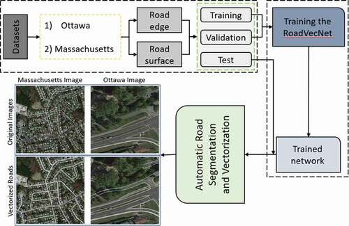
This study implemented an interlinked UNet networks called RoadVecNet for simultaneous road surface segmentation and vectorization from HRSI. The main steps for applying the suggested method listed are as follows: (i) dataset preparation was performed to conduct the testing, training, and validation imagery for road surface segmentation and vectorization; (ii) the presented framework was then trained and validated based on the training and validation images; (iii) the trained framework was then applied to the test images to produce road surface and vectorized road maps; (iv) the performance of the presented framework was evaluated on the basis of the evaluation metrics, and the results were compared with some preexisting deep learning methods.

2.1. RoadVecNet architecture

An overview of the suggested RoadVecNet framework is shown in Figure 1. The proposed network comprises the road surface segmentation and road vectorization networks (Figure 1). Each UNet model includes a contracting encoder arm where the resolution decreases, and the feature depth increases and an expanding decoder arm where the resolution increases, and the feature depth decreases. We utilized filters sizes of 32, 64, 128, and 256 to consider the number of feature maps in encoder–decoder. The skip connections characteristic of the U-Net framework (Ronneberger, Fischer, and Brox 2015) connect each upsampled feature map at the decoder arm to the encoder’s arm with an identical spatial resolution. Accordingly, the probability map that indicates the likelihood of every road and non-road pixel is obtained with the sigmoid classifier.

Figure 1. Flowchart of the RoadVecNet framework containing (a) road surface segmentation and (b) road vectorization UNet networks

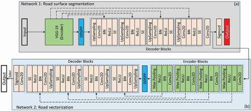
1) Road surface segmentation architecture: The detailed configuration of this network is shown in Figure 2(a). This network was first applied to detect the road surface, which is categorized into two: road and background categories. In this network, pre-trained VGG-19 (Simonyan and Zisserman 2014) was used as an encoder because VGG-19 can be easily transferred to another task, given that it has formerly learned features from ImageNet. The key advantages of adopting the VGG-19 network are as follows: (1) its design is identical to UNet, making it easier to combine with UNet, and (2) it will allow much deeper networks to produce superior output segmentation and vectorization results. We also used the DDSPP module to extract high-resolution feature maps and capture contextual information within the architecture and the SE module to pass more relevant data and reduce redundant ones. Every block in the decoder part implements a $2\times 2$ bilinear upsampling on the input features to double the dimension of the input feature maps. This avoids artifacts and the use of slow deconvolution layer and hence decreases the number of learning parameters, which it also contributes to a faster total training and inference time. Then, the proper skip connections of the encoder feature maps to the output feature maps are concatenated. Thereafter, two $3\times 3$ convolutional layers were applied, followed by batch normalization (BN) and Rectified Linear Unit (ReLU) function. The distribution of activations varies in the intermediate layers during the training step, which is a problem. This issue slows down the training phase because every layer in every training phase must learn to adjust to a new distribution. Thus, BN (Ioffe and Szegedy 2015), which standardizes the inputs to a layer in the network by subtracting the batch mean and dividing by the batch standard deviation, is used to improve the stability of a neural network. The speed of a neural network’s training process can be accelerated by BN (Ioffe and Szegedy 2015). Furthermore, the model’s performance is improved in some cases due to the modest regularization influence. Subsequently, the SE module was used, and the mask was generated by applying a convolutional layer with the sigmoid function. In remote sensing imagery, the road samples face the class imbalance issue because of the skewed dispensation of ground objects (Abdollahi, Pradhan, and Alamri 2020). The cross-entropy loss does not adequately account for the imbalanced classes because it is calculated by summing up all of the pixels. A typical approach for considering the imbalanced classes is to use a weighting factor (Eigen and Fergus 2012). The class loss is weighted using median frequency balancing by the ratio of the training set’s median class frequency and the real class frequency (Eigen and Fergus 2012). The presentation of a weighting factor between the simple and the hard samples is the same; however, it balances the value of positive and negative samples. Therefore, the focal loss function was implemented by Lin et al. (2017) to lessen the burden of simple samples, allowing them to focus more on the hard samples. We used the focal loss weighted by the median frequency balancing (MFB_FL) to address the imbalance issue of the training data and train the road surface segmentation network that is denoted as follows:

(1) $MFB\mathrm{\_}F{L}_{seg}(g,f(o),{\delta }_1)=\alpha (1-l_c(I_i^j){)}^{\gamma }.BC{E}_{seg}$(1)

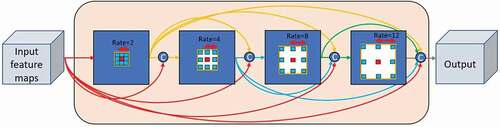
Figure 2. DDSPP structure. Each dilated convolutional layer’s output is concatenated (C) with the input feature map and then fed to the subsequent dilated layer

where

(2) $BC{E}_{seg}=-\sum _{i=1}^S\sum _{j=1}^P\sum _{c=1}^C{w}_c\cdot (g_i^j=C)log{l}_c(I_i^j)$(2)

$w_c=\frac{median(m_c|c\in C)}{m_c}$

,

where$median(m_c)$ is the median value of every $m_c$, $m_c$ is the modulation of pixels in class c, $w_c$ is the class weight, $f(I_i^j)$ is the output of the final convolutional layer at pixel $I_i^j$, $g_i^j$ is the surface ground truth label, $I_i^j$ is the $jth$ pixel in the $ith$ patch, $C$ is the amount of classes, $P$ is the amount of pixels in every patch, $S$ is the batch size, ${\delta }_1$ denotes the road segmentation model parameters, and $l_c(I_i^j)$ is defined as the road surface likelihood of pixel $I_i^j$

(3) $l_c(I_i^j)=\frac{exp(f_c(I_i^j))}{\sum _{l=1}^{c}exp(f_l(I_i^j))}.$(3)

2) Road vectorization architecture: The detailed configuration of this network is shown in Figure 2(b). This network was then implemented to vectorize roads and extract the accurate width and location of the road network. The architecture has a similar architecture as the road surface segmentation architecture that has a contracting arm, expanding arm, skip connections, and sigmoid layer; however, it is much smaller than the road surface segmentation model. A relatively small architecture was chosen for this part for the following reasons. First, the training network has fewer positive pixels (vectorized road pixels) compared with the road segmentation framework. Thus, applying a relatively deep network may cause overfitting. In addition, the feature maps generated by the final convolutional layer in the decode arm of the road segmentation framework have fewer complex backgrounds compared with the original image. A relatively small architecture is sufficient to deal with the vectorization task. In Figure 2, the inputs of the vectorization model are the feature maps generated by the final convolutional layer of the decoder arm in the road segmentation model. In every encoder block, two $3\times 3$ convolutional layers were implemented, followed by batch normalization and ReLU. Thereafter, the SE block is used to enhance the feature map’s quality. Then, a$2\times 2$ max-pooling layer with stride 2 was applied to decrease the spatial dimension of the feature maps. All the components in the decoder arm are comparable to those of the decoder arm of the road segmentation network. To train the road vectorization model, its MFB_FL is denoted as follows:

(4) $MFB\mathrm{\_}F{L}_{vec}(y,h(I),{\delta }_2)=\alpha (1-l_c(f(I_i^j)){)}^{\gamma }.BC{E}_{vec}$(4)

where

(5) $BC{E}_{vec}=-\sum _{i=1}^S\sum _{j=1}^P\sum _{c=1}^C{w}_c\cdot (y_i^j=C)log{l}_c(f(I_i^j))$(5)

where $y_i^j$ is the vectorized ground truth label, $h(f(I_i^j))$ is the output of the final convolutional layer in the road vectorization network, $f(I_i^j)$ is the output of the final convolutional layer at pixel $I_i^j$ in the road segmentation model, $C$ is the amount of classes, $P$ is the amount of pixels in every patch, $S$ is the batch size, ${\delta }_2$ denotes the road vectorization network parameters, and $l_c(f(I_i^j))$ is denoted as the vectorized road likelihood of pixel $I_i^j$.

(6) $l_c(f(I_i^j))=\frac{exp(h_c(f(I_i^j)))}{\sum _{l=1}^{c}exp(h_1(f_{\hspace{0.17em}}(I_i^j)))}.$(6)

We employed an end-to-end strategy to concurrently train the proposed road segmentation network and road vectorization network and utilized a distinct training dataset for every subtask. Moreover, we used the main RGB (red, green, and blue) images and the corresponding ground truth surface images for the road surface segmentation task and the main images and its corresponding ground truth vectorized images for the road vectorization task. Finally, the overall loss function in RoadVecNet, which is a combination of losses (1) and (3), can be expressed as follows:

(7) $\begin{array}{r}MFB\mathrm{\_}FL({\delta }_1+{\delta }_2)=MFB\mathrm{\_}F{L}_{seg}(g,f(o),{\delta }_1)\\ +MFB\mathrm{\_}F{L}_{vec}(y,h(I),{\delta }_2)=\\ \alpha (1-l_c(I_i^j){)}^{\gamma }.BC{E}_{seg}+\alpha (1-l_c(f(I_i^j)){)}^{\gamma }.BC{E}_{vec}\end{array}$(7)

where the last convolutional layer’s output in the road vectorization network is $h(f(\cdot ))$, and the last convolutional layer’s output in the road segmentation model is $f(\cdot )$. The focal loss is parameterized by $\gamma$ and $\alpha$, and it controls the degree of downweighting of easy examples and the class weights, respectively. The FL simplifies to BCE when $\gamma$=0. In this work, we set the values for $\gamma =2$ and $\alpha =0.25$ because the degree of concentrating on hard and easy samples can be increased by higher values of $\gamma$ and lower values of $\alpha$.

2.2. SE module

The SE module (Hu, Shen, and Sun 2018) was used to improve the model’s representation power by a context gating mechanism and attain a clear relationship between the convolutional layer channels. The module encodes feature maps by allocating a weight for every channel in the feature map. The SE module includes two major parts, called squeeze and excitation. The first operation is squeeze. The input feature maps to SE block are accumulated to generate a channel descriptor by applying global average pooling (GAP) of the entire context of channels. We have $X_d^{up}=[X_1^{up},X_2^{up},\dots ,X_F^{up}]$, in which the input data to the SE module are $X_f^{up}\in R^{W\times H}$, and the spatial squeeze is calculated as follows:

(8) $z_f=F_{sq}(X_f^{up})=\frac{1}{H\times W}\sum _i^H\sum _j^W{X}_f^{up}(i,j)$(8)

where $H\times W$ is the size of this channel, $X_f^{up}(i,j)$ is a spatial location of the $f^{th}$ channel, and $F_{sq}$ is the spatial squeeze module. The second operation is excitation, which takes the global information produced in the squeeze stage. This operation includes two fully connected (FC) layers. The pooled vector is first encoded and then decoded to shape $1\times 1\times \frac{F}{r}$ and $1\times 1\times F$, respectively, to generate an excitation vector as $s=F_{ex}(z;W)=\sigma (W_2\mathrm{\Re }(W_{1}z))$, where $W_1\in R^{\frac{F}{r}\times F}$ denotes the parameters of the initial FC layer $R^{F\times \frac{F}{r}}$, $r$ is the reduction ratio, $\mathrm{\Re }$ is ReLU, and $\sigma$ denotes the sigmoid function. The output of the SE block is generated as ${\tilde{X}}_f^{up}=F_{scale}(X_f^{up},z_c)=s_c{X}_f^{up}$, where ${\tilde{X}}_d^{up}=[{\tilde{X}}_1^{up},{\tilde{X}}_2^{up},\dots ,{\tilde{X}}_F^{up}$ is a channel-wise multiplication between the channel attention, $s_c$ is the scale factor, and $F_{scale}$ is the input feature map.

2.3. DDSPP module

In this work, the DDSPP module was performed on the feature maps generated by the encoder arms to elicit further multi-scale contextual information and produce a greater number of scale features over a broader range. Atrous spatial pyramid pooling (ASPP) was first utilized in DeepLab (Chen et al. 2017) to enhance the suggested networks’ performance. ASPP is a mixture of spatial pyramid pooling and atrous convolution with various atrous rates. This tool is effective in adjusting the receptive field to catch multi-scale information and in controlling the resolution of the features computed by deep learning networks. In particular, ASPP includes (a) an image-level feature that is generated by global average pooling and (b) one convolution with a $1\times 1$ filter size and four parallel convolutions of a $3\times 3$ filter size with different rates of 2, 4, 8, and 12, as illustrated in Figure 2. Then, bilinear upsampling was applied to upsample the outcoming features from the entire branches to the input size and concatenated and underwent another convolution with $1\times 1$. However, we used a new module named DDSPP (Yang et al. 2018), which combines the benefit of cascaded modules with atrous convolution and ASPP to produce more scale features over a broader range and exploit further multi-scale contextual features. The receptive field for atrous convolution can be defined as follows:

(9) $F=[(K-1)(R-1)+K]\times [(K-1)(R-1)+K]$(9)

where $R$ is the rate, and $k$ is the convolution kernel size. For example, when R= 2 and K= 3, the F is then equal to 5 × 5. However, we can have a bigger receptive field and can create feature pyramids with a more denser scale variability by using dense connections between stacked dilated layers. Assuming that we have two convolutional operations with K₁ and K₂ kernel sizes, the receptive field can be defined as follows:

(10) $F=(K_1+K_2-1)\times (K_1+K_2-1)$(10)

The new receptive field size will result in 13 × 13 when the rates are 2 and 4.

2.4. Inference stage

The road surface segmentation and road vectorization can be concurrently implemented through the proposed RoadVecNet in the inference stage (Figure 2). A probability road map was achieved by using the road segmentation network. Then, the road vectorization network transformed the features maps of the final convolutional layer generated by using a road segmentation model into vector-based possibility maps in the inference stage. Finally, the Sobel algorithm was applied to achieve a complete and smooth road vectorization network with precise road width information (Vincent and Folorunso 2009). The Sobel algorithm is an instance of the gradient approach. In the gradient method, the edges are detected by looking for the minimum and maximum in the image’s initial derivative. The Sobel method computes an estimation of the image intensity gradient function and is a discrete differentiation method (Vincent and Folorunso 2009).

3. Experiments and Assessment

The experimental settings in the suggested approach are first introduced in this section. Subsequently, we described the Massachusetts and Ottawa datasets used for road segmentation and vectorization. Next, the evaluation metrics and quantitative results achieved by the proposed approach and other comparative techniques for road surface segmentation and road vectorization tasks are described.

3.1. Experimental setting

We utilized some data augmentation strategies, such as flipping the images vertically and horizontally as well as rotating them 90^°, 180^°, and 270^° to expand the size of our training and validation sets and train a proper model. Moreover, to dominate the overfitting difficulty, we appended a dropout of 0.5 (Srivastava et al. 2014) to the deeper convolutional layers of the road segmentation network and road vectorization network. A computationally affordable yet strong regularization to the model can be provided using this strategy. Adaptive moment estimation (Adam) optimizer with 0.001 learning rate was also utilized in this work to learn the model parameters, such as weights and biases via optimizing the loss function. The presented RoadVecNet was trained with batch size 2 from scratch except the backbone network that we used as the pretrained one. The trained network was then implemented on the test data for road surface segmentation and road vectorization. We implemented the optimization of the networks for 100 epochs through the datasets until no more performance improvements were seen. We applied the suggested network for road surface segmentation and road vectorization on a GPU Nvidia Quadro RTX 6000 with a memory of 24 GB and a computing capability of 7.5 under Keras framework with Tensorflow backend.

3.2. Dataset descriptions

Two types of remote sensing datasets called Massachusetts road imagery (Mnih 2013) containing aerial images with 0.5 m spatial resolution and Ottawa road imagery (Liu et al. 2018) containing Google Earth images with 0.21 m spatial resolution were used to test the proposed network on the road segmentation and vectorization. We selected these two different datasets, which contain various road width pixels, to show the proposed architecture’s superiority in road segmentation and vectorization. Each dataset includes two sub-datasets, namely, road surface segmentation and road vectorization. The detailed information of each dataset is highlighted as follows:

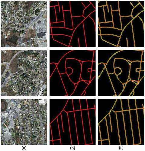
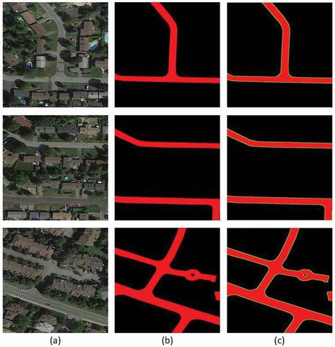
1) Massachusetts datasets: In this dataset, we used 766 images, which are split into 690 training, 48 validation, and 28 test images with a dimension of 512 × 512 and road width of approximately 6–9 pixels. Figure 3 demonstrates some samples of the original images in the first column, the corresponding reference map in the second column, and a superposition between vectorized road and road segmentation ground truth maps in the last column.

Figure 3. Demonstration of three representative imagery, their segmentation ground truth, and vectorized ground truth maps for the Massachusetts road imagery. (a), (b), and (c) illustrate the original RGB imagery, corresponding segmentation ground truth maps, and superposition between vectorized and segmentation ground truth maps, respectively

2) Ottawa datasets: We utilized 652 images divided into 598 training, 34 validation, and 20 test images with a dimension of 512 × 512 and road width of almost 24–28 pixels. Figure 4 illustrates some examples of the main imagery, the corresponding reference map, and the superposition between vectorized road and road segmentation ground truth maps in the first, second, and last columns, respectively.

Figure 4. Demonstration of three representative imagery and their segmentation ground truth and vectorized ground truth maps for the Ottawa road imagery. (a), (b), and (c) demonstrate the main RGB images, corresponding segmentation ground truth maps, and superposition between vectorized and segmentation ground truth maps, respectively

3.3. Evaluation factors

We utilized F1 score (14) and Matthew correlation coefficient (MCC) factors to assess the ability of the presented RoadVecNet for road surface segmentation and vectorization. The IOU factor (13) is calculated by dividing the total number of mutual pixels between the real and the classified masks by the total number of present pixels in both masks. A correlation coefficient between the predicted and the identified binary classification was denoted as MCC (15), providing a value between −1 and +1, and a mixture of the recall (12) and precision (11) factors was denoted as F1 score (Abdollahi, Pradhan et al. 2020). These measurement metrics can be computed from the amount of false negative (FN), false positive (FP), true positive (TP), and true negative (TN) pixels as follows:

(11) $Precision=\frac{TP}{TP+FP}$(11)

(12) $Recall=\frac{Tp}{TP+FN}$(12)

(13) $IOU=\frac{TP}{TP+FP+FN}$(13)

(14) $\begin{array}{cc}F1& score\end{array}=\frac{2\times Precision\times Recall}{Precision+Recall}$(14)

(15) $MCC=\frac{TP.TN-FP.FN}{\sqrt{(TP+FP)(TP+FN)(TN+FP)(TN+FN)}}$(15)

A buffet width $p$ should be defined because of the differences between the real road width map and the manually annotated road width map (Shao et al. 2021). The matching areas $TP$ are defined as areas in the anticipated results that are within a $p$ pixel range. We followed the work of Shao et al. (2021) to set the buffer width $p=2$. The same indices were used to assess the outcomes of vectorized roads.

3.4. Qualitative comparison of road surface segmentation

We compared the presented RoadVecNet architecture with some other state-of-the-art classification-based deep learning networks to investigate the capability of the network in road surface segmentation from HRSI. Examples of these networks are as follows: UNet architecture provided by Ronneberger, Fischer, and Brox (2015); SegNet network implemented by Badrinarayanan, Kendall, and Cipolla (2017); DeepLabV3 framework performed by Chen et al. (2017); VNet model applied by Abdollahi, Pradhan, and Alamri (2020); ResUNet provided by Diakogiannis et al. (2019); and FCN architecture developed by Long, Shelhamer, and Darrell (2015). For denoting segmentation, we utilized the suffix “-S” after each method’s name. The visualization outcomes obtained by the presented RoadVecNet architecture and other comparative networks for road surface segmentation from the Massachusetts and Ottawa datasets are demonstrated in Figures 5, 6, and 7. The figures illustrate that the SegNet-S, ResUNet-S, and DeepLabV3-S networks were sensitive to the barriers of trees and shadows and predicted more FN pixels (depicted as blue color) and FP pixels (depicted as green color), thereby producing low-quality road segmentation maps for both datasets. Meanwhile, the FCN-S, UNet-S, and VNet-S architectures could improve the results and generate more coherent and satisfactory road segmentation maps. However, none of the abovementioned models achieved better qualitative results than Ours-S. Ours-S could generate high-resolution road segmentation maps for both datasets by alleviating the effect of obstacles, predicting less FP pixels, and preserving the road border information. The reason is that we used the DDSPP module to create feature pyramids with more denser scale variability and a bigger receptive field. We also utilized the SE module to extract more valuable information by considering the interdependencies between feature channels. In addition, we applied the MFB_FL loss function to overcome highly unbalanced datasets and allow more attention on the hard samples. Therefore, we could obtain more constant and smoother road segmentation and vectorization results.

Figure 5. Visual performance attained by Ours-S against the other comparative networks for road surface segmentation from the Massachusetts imagery. The cyan, green and blue colors denote the TPs, FPs, and FNs, respectively

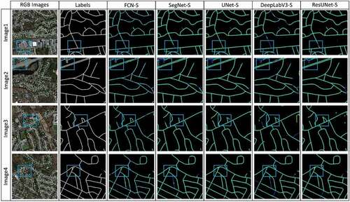
Figure 6. Visual performance attained by the comparative networks for road surface segmentation from the Ottawa imagery. The cyan green, and blue colors denote the TPs, FPs, and FNs, respectively

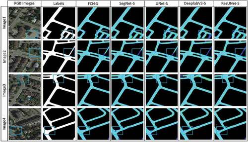
Figure 7. Visual performance attained by Ours-S against VNet-S network for road surface segmentation from the Ottawa and Massachusetts imagery. The cyan, green, and blue colors denote the TPs, FPs, and FNs, respectively

3.5. Qualitative comparison of road vectorization

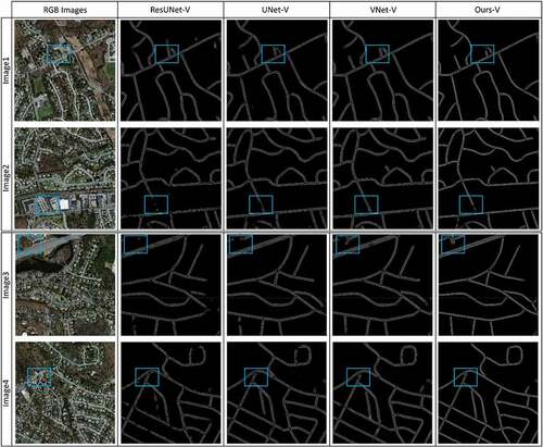
Here, we compared the results attained by the presented RoadVecNet architecture for road vectorization from the Massachusetts and Ottawa datasets with the same comparative deep learning methods applied in the road surface segmentation part, such as UNet architecture (Ronneberger, Fischer, and Brox 2015), DeepLabV3 framework (Chen et al. 2017), SegNet network (Badrinarayanan, Kendall, and Cipolla 2017), VNet applied by Abdollahi, Pradhan, and Alamri (2020), ResUNet provided by Diakogiannis et al. (2019), and FCN (Long, Shelhamer, and Darrell 2015). We utilized the suffix “-V” after every approach’s name to denote road vectorization. Figures 9 and 10 demonstrate the comparison outcomes of various approaches and the presented RoadVecNet for road vectorization in visual performance for Ottawa imagery. The vectorized road ground truth map is also included in the second column of the figure to better display the contrast influences. We also used blue rectangular boxes in the figures to show the FP and FN pixels for facilitating comparison. Figures 8 and 9 illustrate that although the FCN-V, SegNet-V ResUNet-V, and DeepLabV3-V architectures could generate relatively complete road vectorization network, they brought in spurs and produced some FPs in the homogenous regions where the road was covered by occlusions and around the intersections, reducing the correctness and smoothness of the road vectorization network. The UNet-V and VNet-V methods could improve the results and generate a complete network of the road vectorization; however, it failed to vectorize the road in the intersection parts and brought in some discontinuity and FPs. Figures 10 and 11 demonstrate the visual performance of the comparative models for Massachusetts imagery. In this dataset, the complexity of obstacles and backgrounds are more, and the road width is less than those in the Ottawa dataset. Accordingly, all the above-mentioned comparative models, including VNet-V, could not accurately vectorize the road, resulting in non-complete and non-smooth vectorized road network, especially for complex backgrounds and intersection areas where they brought in more discontinuity and FPs. By contrast, Ours-V could detect complete and non-spur vectorized road network even from the Massachusetts dataset with narrow road width and complex backgrounds. Our vectorized road map is more similar to the actual ground truth vectorized road than the other comparative models.

Figure 8. Comparison outcomes of various approaches for road vectorization in visual performance for Ottawa imagery. The first and second columns demonstrate the original RGB and corresponding reference imagery, respectively. The third, fourth, fifth, sixth, and last columns demonstrate the results of FCN-V, SegNet-V, UNet-V, DeepLabV3-V, and ResUNet-V. More details can be seen in the zoomed-in view

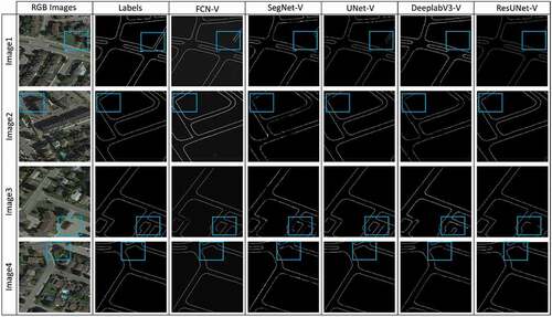
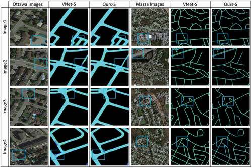
Figure 9. Comparison of the outcomes of the VNet-V approach and Ours-V for road vectorization in terms of visual performance for Ottawa imagery. The first and second columns demonstrate the original RGB and corresponding reference imagery, respectively. The third and fourth columns demonstrate the results of VNet-V and Ours-V. More details can be seen in the zoomed-in view

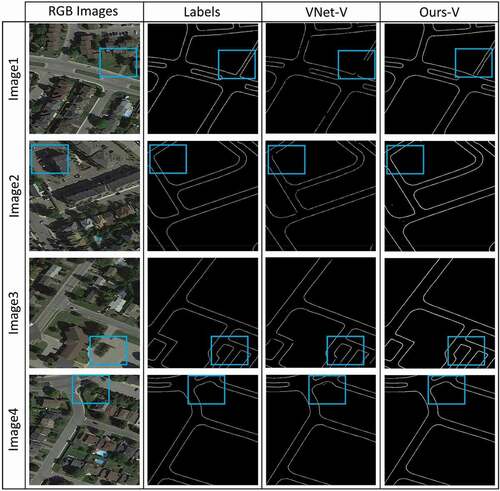
Figure 10. Comparison of the outcomes of various approaches for road vectorization in terms of visual performance for Massachusetts imagery. The first and second columns demonstrate the original RGB and corresponding reference imagery, respectively. The third, fourth, and fifth columns demonstrate the results of FCN-V, SegNet-V, and DeepLabV3-V, respectively. More details can be seen in the zoomed-in view

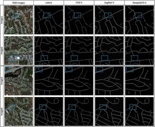
Figure 11. Comparison outcomes of our approach and the other comparative models for road vectorization in visual performance for Massachusetts imagery. The first column demonstrates the original RGB imagery. The second, third, fourth, and last columns demonstrate the results of ResUNet-V, UNet-V, VNet-V, and Ours-V, respectively. More details can be seen in the zoomed-in view

4. Discussion

We obtained the quantitative calculations for the presented technique and other comparative networks applied to the Massachusetts and Ottawa datasets for road segmentation, which are summarized in Tables 1 and 2, respectively. The first four columns in both tables are the performance of four test sample imagery, and the final column is the average accuracy of the whole test imagery. The bold value is the best in the F1 score metric, while the underlined values are the second-best. Tables 1 and 2 illustrate that Ours-S, along with other comparative convolutional networks, could attain satisfactory outcomes for road segmentation from both datasets. However, the DeepLabV3-S, ResUNet-S, and SegNet-S architectures achieved the lowest F1 score accuracy with 85.83%. 86.97%, and 87% for Massachusetts and 90.54%, 90.72%, and 91.48% for Ottawa. The SegNet-S model could slightly improve the accuracy because it utilizes the max-pooling indices at the encoder and corresponding decoder paths to upsample the layers in the decoding process. The model does not need to learn the upsampling weights again because this function makes the training process more straightforward.

Table 1. Percentage of F1 score, MCC, and IOU attained by Ours-S and other comparative networks for road segmentation from Massachusetts imagery. The bold and underline F1 scores demonstrate the best and second-best, respectively

		Image1	Image2	Image3	Image4	Average
FCN-S	F1 score	0.9104	0.9117	0.9028	0.9007	0.9064
	MCC	0.9008	0.9037	0.8910	0.8901	0.8964
	IOU	0.8338	0.8360	0.8212	0.8176	0.8272
SegNet-S	F1 score	0.8680	0.8909	0.8701	0.8511	0.8700
	MCC	0.8554	0.8838	0.8573	0.8324	0.8572
	IOU	0.7654	0.8017	0.7686	0.7394	0.7688
UNet-S	F1 score	0.9128	0.9141	0.9075	0.9073	0.9104
	MCC	0.9017	0.9057	0.8984	0.8942	0.9000
	IOU	0.8378	0.8570	0.8289	0.8286	0.8381
VNet-S	F1 score MCC IOU	0.9122 0.9023 0.8385	0.9192 0.9108 0.8504	0.9084 0.8965 0.8322	0.9173 0.9067 0.8473	0.9145 0.9040 0.8421
ResUNet-S	F1 score MCC IOU	0.8632 0.8493 0.7593	0.8882 0.8806 0.7988	0.8668 0.8539 0.7649	0.8609 0.8453 0.7557	0.8697 0.8572 0.7696
DeeplabV3-S	F1 score	0.8564	0.8798	0.8468	0.8503	0.8583
	MCC	0.8383	0.8693	0.8294	0.8303	0.8418
	IOU	0.7475	0.7839	0.7330	0.7382	0.7507
Ours-S	F1 score	0.9243	0.9239	0.9282	0.9240	0.9251
	MCC	0.9143	0.9168	0.9190	0.9128	0.9157
	IOU	0.8574	0.8740	0.8641	0.8568	0.8631

Table 2. Percentage of F1 score, MCC, and IOU attained by Ours-S and other comparative networks for road segmentation from Ottawa imagery. The bold and underline values demonstrate the best and second-best, respectively

		Image1	Image2	Image3	Image4	Average
FCN-S	F1 score	0.8829	0.9150	0.9375	0.9282	0.9159
	MCC	0.8453	0.8887	0.9103	0.8796	0.8810
	IOU	0.7888	0.8415	0.8803	0.8641	0.8437
SegNet-S	F1 score	0.8816	0.9302	0.9371	0.9103	0.9148
	MCC	0.8432	0.9053	0.9102	0.8572	0.8790
	IOU	0.7867	0.8676	0.8797	0.8336	0.8419
UNet-S	F1 score	0.8849	0.9329	0.9321	0.9231	0.9183
	MCC	0.8477	0.9108	0.9028	0.8711	0.8831
	IOU	0.7921	0.8722	0.8709	0.8554	0.8477
VNet-S	F1 score MCC IOU	0.8933 0.8597 0.8072	0.9294 0.9070 0.8681	0.9390 0.9137 0.8850	0.9191 0.8678 0.8502	0.9202 0.8870 0.8526
ResUNet-S	F1 score MCC IOU	0.8761 0.8137 0.7484	0.9160 0.8887 0.8450	0.9372 0.9110 0.8818	0.8995 0.8159 0.7949	0.9072 0.8573 0.8175
DeeplabV3-S	F1 score	0.8731	0.9274	0.9330	0.8884	0.9054
	MCC	0.8101	0.9016	0.9027	0.8229	0.8593
	IOU	0.7427	0.8627	0.8725	0.7759	0.8135
Ours-S	F1 score	0.8992	0.9412	0.9434	0.9520	0.9340
	MCC	0.8666	0.9202	0.9186	0.9190	0.9061
	IOU	0.8152	0.8869	0.8909	0.9062	0.8748

Tables 1 and 2 also show that the VNet-S framework was the second-best approach in road surface segmentation, with 91.45% for Massachusetts and 92.02% for Ottawa. By contrast, the accuracy of the F1 score metric for Ours-S was higher than all the comparative approaches. In fact, the presented model could improve the F1 score accuracy by 1.06% for Massachusetts and 1.38% for Ottawa compared with the VNet-S network, which was the second-best model. Furthermore, we compared the quantitative results achieved by the proposed model with more deep learning-based models, such as CNN-based segmentation method (Wei, Zhang, and Ji 2020), road structure-refined CNN (RSRCNN) technique (Wei, Wang, and Xu 2017), and FCNs approach (Zhong et al. 2016) applied for road segmentation from Massachusetts imagery. The presented method was built and evaluated on an experimental dataset, while the outcomes for the other three works were taken from a previously published study. The F1 score accuracy achieved by the CNN-based approach, RSRCNN, and FCNs were 82%, 66.2%, and 68%, respectively, while that of Ours-S approach is 92.51%. The results confirmed that the more supervised information in the presented model obtains better outcomes against the other preexisting deep learning approaches in road surface segmentation from the HRSI.

We calculated the F1 score and MCC metrics to better probe the capability of Ours-V and other comparative models in road vectorization. The qualitative outcomes for the Ottawa (Google Earth) and Massachusetts (aerial) imagery are demonstrated in Table 3 and Table 4, respectively. Table 3 and Table 4 show that the VNet-V could achieve satisfactory results for road vectorization from the Ottawa imagery with 91.27% F1 score accuracy, which could improve the results of other comparative models, such as FCN-V, DeepLabV3-V, ResUNet-V, UNet-V, and SegNet-V, and it was ranked as the second-best model. Nevertheless, this method could not perform well in road vectorization using the Massachusetts imagery (Table 4) and predicted more FPs and less FNs, resulting in less F1 score accuracy with 83.73%, which is not very good. This phenomenon is attributed to the aerial images that have more complex backgrounds and occlusions, and the road width is narrow. The other methods that could not achieve a higher F1 score accuracy than VNet-V for Ottawa images could not obtain a higher accuracy for Massachusetts images as well. By contrast, Ours-V was able to achieve better results than others for both datasets. Ours-V achieved F1 score accuracy rates of 92.41% and 89.24% for Ottawa and Massachusetts imagery, respectively. Ours-V could improve the results of VNet-V (second-best method) to 1.14% for Ottawa and 5.51% for Massachusetts, which confirmed its validity for road vectorization from Google Earth and Arial imagery.

Table 3. Percentage of F1 score and MCC attained by Ours-V and other comparative networks for road vectorization from the Ottawa imagery. The bold and underline values denote the best and second-best, respectively

		Image1	Image2	Image3	Image4	Average
FCN-V	F1 score	0.8643	0.9017	0.8893	0.8893	0.8862
	MCC	0.8551	0.8953	0.8825	0.8821	0.8788
SegNet-V	F1 score	0.8622	0.8702	0.8820	0.8776	0.8730
	MCC	0.8563	0.8658	0.8782	0.8722	0.8681
UNet-V	F1 score	0.8999	0.9134	0.9072	0.9288	0.9123
	MCC	0.8931	0.9076	0.9015	0.9241	0.9066
DeeplabV3-V	F1 score	0.8566	0.8699	0.8804	0.8742	0.8703
	MCC	0.8513	0.8650	0.8763	0.8695	0.8655
VNet-V	F1 score MCC	0.9045 0.8985	0.9129 0.9071	0.9038 0.8973	0.9297 0.9254	0.9127 0.9070
ResUNet-V	F1 score MCC	0.8614 0.8529	0.8734 0.8659	0.8839 0.8771	0.8874 0.8807	0.8765 0.8691
Ours-V	F1 score	0.9203	0.9237	0.9164	0.9358	0.9241
	MCC	0.9149	0.9187	0.9110	0.9315	0.9190

Table 4. Percentage of F1 score and MCC attained by Ours-V and other comparative networks for road vectorization from Massachusetts imagery. The bold and underline values denote the best and second-best, respectively

		Image1	Image2	Image3	Image4	Average
FCN-V	F1 score	0.7982	0.8350	0.8204	0.8503	0.8260
	MCC	0.8004	0.8273	0.8095	0.8510	0.8221
SegNet-V	F1 score	0.7917	0.8326	0.8047	0.8424	0.8179
	MCC	0.7763	0.8232	0.7911	0.8333	0.8060
UNet-V	F1 score	0.8129	0.8458	0.8237	0.8514	0.8335
	MCC	0.7994	0.8478	0.8244	0.8421	0.8284
DeeplabV3-V	F1 score	0.7539	0.8263	0.7749	0.8237	0.7947
	MCC	0.7350	0.8176	0.7586	0.8114	0.7807
VNet-V	F1 score MCC	0.8206 0.8069	0.8470 0.8388	0.8208 0.8083	0.8619 0.8535	0.8373 0.8268
ResUNet-V	F1 score MCC	0.7771 0.7596	0.8307 0.8218	0.7814 0.7653	0.8298 0.8180	0.8047 0.7911
Ours-V	F1 score	0.8854	0.8834	0.8878	0.9129	0.8924
	MCC	0.8762	0.8754	0.8794	0.9066	0.8844

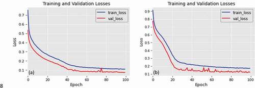
The average F1 score accuracy attained by our approach and other comparative approaches in road surface segmentation and road vectorization from both datasets is plotted in Figure 12(a,b), respectively. The approaches and the average percentage of the F1 score metric are shown in the horizontal and vertical axes, respectively. Figure 12 depicts that the Ours-S and Ours-V methods achieved the highest F1 score, affirming the superiority of the proposed technique for road vectorization from Google Earth and Arial imagery. Figure 13(a,b) display the training and validation losses of the presented approach over 100 epochs for Ottawa and Massachusetts imagery, respectively. Based on the decrease in model loss, the method has learned efficient features for road surface segmentation and vectorization. The training and validation losses are close together in the learning curve for both datasets. The model reduced over-fitting, and the variance of the method is negligible.

Figure 12. Average percentage of the F1 score metric of our method and other methods for road surface segmentation (a) and road vectorization (b) from Ottawa and Massachusetts imagery

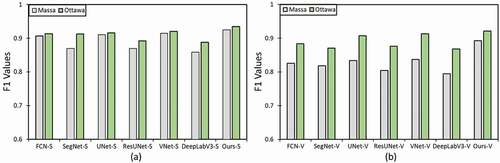
Figure 13. Performance of the proposed model for road segmentation and vectorization through training epochs: training and validation losses for the (a) Ottawa and (b) Massachusetts datasets

4.1. Ablation study

We conducted some tests to see how different settings affected the model’s performance in road surface segmentation and vectorization. In this case, we used PSPNet backbone (Zhao, Shi et al. 2017), stochastic gradient descent with a 0.01 learning rate, and batch size of 4. The quantitative results for both tasks are shown in Table 5. Meanwhile, the visualization results for road segmentation and vectorization tasks are depicted in Figures 14 and 15, respectively. Table 5 illustrates that the accuracy of the F1 score decreased to 91.77% and 87.75% for road segmentation and 90.02% and 85.32% for road vectorization for the Massachusetts and Ottawa images, respectively, after changing some settings. Figures 14 and 15 also show that the proposed model brought in spurs and produced some FPs in the homogenous regions, thereby considerably decreasing the smoothness of the road vectorization network.

Figure 14. Visual performance attained by Ours-S network for road surface segmentation from the Ottawa and Massachusetts imagery after changing several settings. The cyan, green, and blue colors denote the TPs, FPs, and FNs, respectively

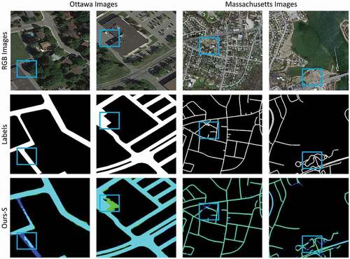
Figure 15. Visual performance attained by Ours-V for road vectorization from the Massachusetts and Ottawa imagery after changing several settings. The blue rectangle shows the predicted FPs and FNs. More details can be seen in the zoomed-in view

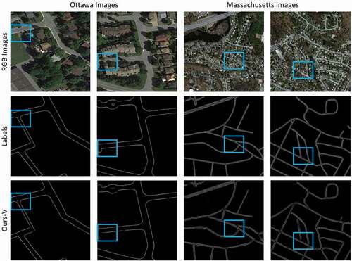
Table 5. Percentage of the F1 score, IOU, and MCC attained by Ours-V network for road segmentation and vectorization from the Massachusetts and Ottawa imagery after changing several settings

Road Segmentation	Ottawa	F1 score	0.9177
		MCC	0.8984
		IOU	0.8684
	Massachusetts	F1 score	0.8775
		MCC	0.8662
		IOU	0.7818
Road Vectorization	Ottawa	F1 score	0.9002
		MCC	0.9048
	Massachusetts	F1 score	0.8532
		MCC	0.8460

4.2. Failure case analysis

In this case, we conducted some failure case analysis by reducing the size of images to 256 × 256 to check the model’s performance on road segmentation and vectorization. Table 6 shows the quantitative results for both tasks. Meanwhile, Figures 16 and 17 illustrate the visualization results for road segmentation and vectorization tasks, respectively. In Table 6, when the size of the image was halved, the accuracy of the F1 score was decreased for road segmentation to 88.87% and 84.44% and road vectorization to 87.02% 81.61% for both Massachusetts and Ottawa imagery, respectively. In addition, Figures 16 and 17 depict that the proposed model showed more noise and confused lanes with each other for road segmentation from both datasets. Moreover, the model produced a non-complete vectorized road network for road vectorization, especially for complicated and intersection areas wherein they brought in more FPs when we decreased the image size. The model could learn considerably less, and the images were distinguished as failure due to overfitting when the image size was reduced. Accordingly, the detection accuracy was greatly diminished. Therefore, reducing the image input size was ineffective for producing high-quality road segmentation and vectorization maps.

Figure 16. Visual performance attained by Ours-S network for road surface segmentation from the Ottawa and Massachusetts imagery after analyzing a failure case. The cyan, green, and blue colors denote the TPs, FPs, and FNs, respectively

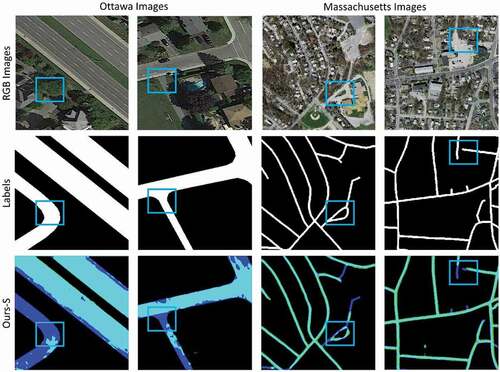
Figure 17. Visual performance attained by Ours-V for road vectorization from the Massachusetts and Ottawa imagery after analyzing a failure case. The blue rectangle shows the predicted FPs and FNs. More details can be seen in the zoomed-in view

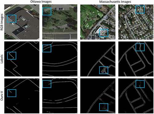
Table 6. Percentage of the F1 score, IOU, and MCC attained by Ours-V network for road segmentation and vectorization from the Massachusetts and Ottawa imagery after analyzing a failure case

Road Segmentation	Ottawa	F1 score	0.8887
		MCC	0.8291
		IOU	0.7997
	Massachusetts	F1 score	0.8444
		MCC	0.8226
		IOU	0.7308
Road Vectorization	Ottawa	F1 score	0.8702
		MCC	0.8637
	Massachusetts	F1 score	0.8161
		MCC	0.8045

5. Conclusion

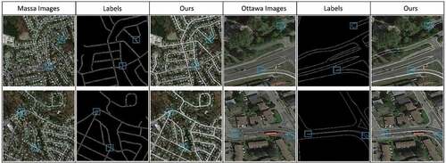
A new interlinked end-to-end UNet framework called RoadVecNet was proposed in this study to simultaneously implement the road surface segmentation and road vectorization. The first network in the RoadVecNet architecture was used to produce feature maps. Meanwhile, the second network was performed to formulate road vectorization. The Sobel method was utilized to achieve a complete and smooth vectorized road with accurate road-width information. Two separate datasets, namely, road surface segmentation and road vectorization datasets, were used to train the model. The advantage of the proposed model was verified with rigorous experiments: 1) Two different road datasets imagery called Ottawa (Google Earth) and Massachusetts (Aerial) datasets, which comprise the original RGB images, corresponding ground truth segmentation maps, and corresponding ground truth vector maps, were employed to test the model for road segmentation and vectorization. 2) In the road surface segmentation tasks, the proposed RoadVecNet could achieve more consistent and smooth road segmentation outcomes than all the comparative models in terms of visual and qualitative performance. 3) In the road vectorization task, RoadVecNet also showed better performance than the other comparative state-of-the-art deep convolutional architectures. Figure 18 demonstrates the vectorized road results overlaid on the original Google Earth and Aerial imagery to prove the overall geometric quality of the road segmentation and vectorization by the model. We calculated the root-mean-square (RMS) of road widths based on the quadratic mean distance between the matched references and extracted widths. The vectorization of the classified outcomes achieved width RMS values of 1.47 and 0.63 m for Massachusetts and Ottawa images, respectively, proving that the proposed model could achieve precise information about road width. Moreover, the proposed network could extract the precise location of the road network because the vectorized road maps are well superimposed with the original imagery. The proposed RoadVecNet model showed robustness against the obstacle to a certain extent; however, it could not segment road and vectorize well, thereby resulting in discontinuity for large and continuous areas of obstacles. These issues are the primary drawbacks of the suggested technique for road surface segmentation and vectorization. Future study can address these constraints by incorporating topological criteria and gap-filling methods into our proposed road extraction and vectorization method to improve its accuracy.

Figure 18. The vectorized road is superimposed with the original Aerial (Massachusetts) and Google Earth (Ottawa) imagery to show the overall geometric quality of vectorized outcomes. The first and second rows demonstrate the Aerial images, and the third and last rows illustrate the Google Earth images. The last column also demonstrates the superimposed vectorized road. More details can be seen in the zoomed-in view

Highlights

• A new RoadVecNet is applied for road segmentation and vectorization simultaneously.

• SE and DDSPP modules are used to improve the accuracy.

• Sobel edge detection method is used to obtain complete and smooth road edge networks

• Two different Massachusetts and Ottawa datasets are used for road vectorization.

• MFB_FL loss function is utilized to overcome highly unbalanced training dataset.

Author contributions

Author Contributions: A.A. carried out the investigations, analyzed the data, and drafted the article; B.P. conceptualized, supervised, visualized, project administered, resource allocated, wrote, reviewed, edited, and reorganized the article; B.P. and A.A.A. effectively enhanced the article, along with the funding. All authors have read and consented to the published version of the article.

Data availability

The Massachusetts and Ottawa datasets and developed code that is uploaded at Github can be downloaded from the online versions at https://www.cs.toronto.edu/~vmnih/data/, https://github.com/gismodelling/RoadVecNet, and https://github.com/yhlleo/RoadNet.

Disclosure statement

No potential conflict of interest was reported by the author(s).

Additional information

Funding

The Centre for Advanced Modelling and Geospatial Information Systems, Faculty of Engineering and IT, University of Technology Sydney funded this research. This research was also supported by Researchers Supporting Project number RSP-2021/14, King Saud University, Riyadh, Saudi Arabia.

References

- Abdollahi, A., and B. Pradhan. 2021. “Integrated Technique of Segmentation and Classification Methods with Connected Components Analysis for Road Extraction from Orthophoto Images.” Expert Systems with Applications 176: 114908. doi:https://doi.org/10.1016/j.eswa.2021.114908.
- Abdollahi, A., B. Pradhan, and A. Alamri. 2020. “VNet: An End-to-end Fully Convolutional Neural Network for Road Extraction from High-resolution Remote Sensing Data.” IEEE Access 8: 179424–179436. doi:https://doi.org/10.1109/ACCESS.2020.3026658.
- Abdollahi, A., B. Pradhan, N. Shukla, S. Chakraborty, and A. Alamri. 2020. “Deep Learning Approaches Applied to Remote Sensing Datasets for Road Extraction: A State-of-the-art Review.” Remote Sensing 12 (9): 1444. doi:https://doi.org/10.3390/rs12091444.
- Badrinarayanan, V., A. Kendall, and R. Cipolla. 2017. “Segnet: A Deep Convolutional Encoder-decoder Architecture for Image Segmentation.” IEEE Transactions on Pattern Analysis and Machine Intelligence 39 (12): 2481–2495. doi:https://doi.org/10.1109/TPAMI.2016.2644615.
- Buslaev, A., S. Seferbekov, V. Iglovikov, and A. Shvets. 2018. “Fully Convolutional Network for Automatic Road Extraction from Satellite Imagery.” In Proceedings of the IEEE Conference on Computer Vision and Pattern Recognition Workshops: 207–210. Salt Lake City, UT, USA.
- Chaudhuri, D., N. Kushwaha, and A. Samal. 2012. “Semi-automated Road Detection from High Resolution Satellite Images by Directional Morphological Enhancement and Segmentation Techniques.” IEEE Journal of Selected Topics in Applied Earth Observations and Remote Sensing 5 (5): 1538–1544. doi:https://doi.org/10.1109/JSTARS.2012.2199085.
- Chen, L., G. Papandreou, I. Kokkinos, K. Murphy, and A. Yuille. 2017. “Deeplab: Semantic Image Segmentation with Deep Convolutional Nets, Atrous Convolution, and Fully Connected Crfs.” IEEE Transactions on Pattern Analysis and Machine Intelligence 40 (4): 834–848. doi:https://doi.org/10.1109/TPAMI.2017.2699184.
- Cheng, G., Y. Wang, S. Xu, H. Wang, S. Xiang, and C. Pan. 2017. “Automatic Road Detection and Centerline Extraction via Cascaded End-to-end Convolutional Neural Network.” IEEE Transactions on Geoscience and Remote Sensing 55 (6): 3322–3337. doi:https://doi.org/10.1109/TGRS.2017.2669341.
- Diakogiannis, F., F. Waldner, P. Caccetta, and C. Wu. 2019. “ResUNet-A: A Deep Learning Framework for Semantic Segmentation of Remotely Sensed Data.” 1–24. https://arxiv.org/abs/1904.00592
- Eigen, D., and R. Fergus. 2012. “Nonparametric Image Parsing Using Adaptive Neighbor Sets.” In 2012 IEEE Conference on Computer Vision and Pattern Recognition: 2799–2806. Providence, RI, USA.
- Gao, X., X. Sun, Y. Zhang, M. Yan, G. Xu, H. Sun, J. Jiao, and K. Fu. 2018. “An End-to-end Neural Network for Road Extraction from Remote Sensing Imagery by Multiple Feature Pyramid Network.” IEEE Access 6: 39401–39414. doi:https://doi.org/10.1109/ACCESS.2018.2856088.
- Hong, Z., D. Ming, K. Zhou, Y. Guo, and T. Lu. 2018. “Road Extraction from a High Spatial Resolution Remote Sensing Image Based on Richer Convolutional Features.” IEEE Access 6: 46988–47000. doi:https://doi.org/10.1109/ACCESS.2018.2867210.
- Hormese, J., and C. Saravanan. 2016. “Automated Road Extraction from High Resolution Satellite Images.” Procedia Technology 24: 1460–1467. doi:https://doi.org/10.1016/j.protcy.2016.05.180.
- Hu, F., G. Xia, J. Hu, and L. Zhang. 2015. “Transferring Deep Convolutional Neural Networks for the Scene Classification of High-resolution Remote Sensing Imagery.” Remote Sensing 7 (11): 14680–14707. doi:https://doi.org/10.3390/rs71114680.
- Hu, J., L. Shen, and G. Sun. 2018. “Squeeze-and-excitation Networks.” In Proceedings of The IEEE Conference on Computer Vision And Pattern Recognition: 7132–7141. Salt Lake City, UT, USA.
- Ioffe, S., and C. Szegedy. 2015. “Batch Normalization: Accelerating Deep Network Training by Reducing Internal Covariate Shift.”448–456. Available from: https://arxiv.org/abs/1502.03167
- Kaur, A., and R. Singh. 2015. “Various Methods of Road Extraction from Satellite Images: A Review.” International Journal of Research 2 (2): 1025–1032.
- Li, P., Y. Zang, C. Wang, J. Li, M. Cheng, L. Luo, and Y. Yu. 2016. “Road Network Extraction via Deep Learning and Line Integral Convolution.” IEEE International Geoscience and Remote Sensing Symposium (IGARSS), Beijing, China, 1599–1602. https://doi.org/10.1109/IGARSS.2016.7729408.
- Li, Y., L. Xu, J. Rao, L. Guo, Z. Yan, and S. Jin. 2019. “A Y-Net Deep Learning Method for Road Segmentation Using High-resolution Visible Remote Sensing Images.” Remote Sensing Letters 10 (4): 381–390. doi:https://doi.org/10.1080/2150704X.2018.1557791.
- Lin, T., P. Goyal, R. Girshick, K. He, and P. Dollár. 2017. “Focal Loss for Dense Object Detection.” Proceedings of the IEEE International Conference on Computer Vision: 2980–2988. Venice, Italy.
- Liu, R., Q. Miao, J. Song, Y. Quan, Y. Li, P. I. Xu, and J. Dai. 2019. “Multiscale Road Centerlines Extraction from High-resolution Aerial Imagery.” Neurocomputing 329: 384–396. doi:https://doi.org/10.1016/j.neucom.2018.10.036.
- Liu, Y., J. Yao, X. Lu, M. Xia, X. Wang, and Y. Liu. 2018. “Roadnet: Learning to Comprehensively Analyze Road Networks in Complex Urban Scenes from High-resolution Remotely Sensed Images.” IEEE Transactions on Geoscience and Remote Sensing 57 (4): 2043–2056. doi:https://doi.org/10.1109/TGRS.2018.2870871.
- Long, J., E. Shelhamer, and T. Darrell. 2015. “Fully Convolutional Networks for Semantic Segmentation.” Proceedings of the IEEE Conference on Computer Vision and Pattern Recognition: 6810–6818. Boston, MA, USA.
- Luo, Y., J. Li, C. Yu, B. Xu, Y. Li, L. Hsu, and N. El-Sheimy. 2019. “Research on Time-correlated Errors Using Allan Variance in a Kalman Filter Applicable to Vector-tracking-based GNSS Software-defined Receiver for Autonomous Ground Vehicle Navigation.” Remote Sensing 11 (9): 1026. doi:https://doi.org/10.3390/rs11091026.
- Maboudi, M., J. Amini, M. Hahn, and M. Saati. 2017. “Object-based Road Extraction from Satellite Images Using Ant Colony Optimization.” International Journal of Remote Sensing 38 (1): 179–198. doi:https://doi.org/10.1080/01431161.2016.1264026.
- Miao, Z., W. Shi, H. Zhang, and X. Wang. 2012. “Road Centerline Extraction from High-resolution Imagery Based on Shape Features and Multivariate Adaptive Regression Splines.” IEEE Geoscience and Remote Sensing Letters 10 (3): 583–587. doi:https://doi.org/10.1109/LGRS.2012.2214761.
- Mnih, V. 2013. “Machine Learning for Aerial Image Labeling.” Ph.D. dissertation, Dept. Comput. Sci., Univ. Toronto, Toronto, ON, Canada.
- Mnih, V., and G. E. Hinton. 2010. “Learning to Detect Roads in High-Resolution Aerial Images.” Berlin, Heidelberg, 210–223. https://doi.org/10.1007/978-3-642-15567-3_16.
- Movaghati, S., A. Moghaddamjoo, and A. Tavakoli. 2010. “Road Extraction from Satellite Images Using Particle Filtering and Extended Kalman Filtering.” IEEE Transactions on Geoscience and Remote Sensing 48 (7): 2807–2817. doi:https://doi.org/10.1109/TGRS.2010.2041783.
- Qiaoping, Z., and I. Couloigner. 2004. “Automatic Road Change Detection and GIS Updating from High Spatial Remotely-sensed Imagery.” Geo-Spatial Information Science 7 (2): 89–95. doi:https://doi.org/10.1007/BF02826642.
- Ronneberger, O., P. Fischer, and T. Brox. 2015. “U-net: Convolutional Networks for Biomedical Image Segmentation.” International Conference on Medical Image Computing and Computer-Assisted Intervention: 234–241. Munich, Germany.
- Saito, S., and Y. Aoki. 2015. “Building and Road Detection from Large Aerial Imagery.” Image Processing: Machine Vision Applications 9405: 94050.
- Ševo, I., and A. Avramović. 2016. “Convolutional Neural Network Based Automatic Object Detection on Aerial Images.” IEEE Geoscience and Remote Sensing Letters 13 (5): 740–744. doi:https://doi.org/10.1109/LGRS.2016.2542358.
- Sarhan, E., E. Khalifa, and A. M. Nabil. 2011. “Road Extraction Framework by Using Cellular Neural Network from Remote Sensing Images.” In 2011 International Conference on Image Information Processing: 1–5. Shimla, India.
- Shao, Z., Z. Zhou, X. Huang, and Y. Zhang. 2021. “MRENet: Simultaneous Extraction of Road Surface and Road Centerline in Complex Urban Scenes from Very High-resolution Images.” Remote Sensing 13 (2): 239. doi:https://doi.org/10.3390/rs13020239.
- Shen, Z., J. Luo, and L. Gao. 2010. “Road Extraction from High-resolution Remotely Sensed Panchromatic Image in Different Research Scales.” In 2010 IEEE International Geoscience and Remote Sensing Symposium: 453–456. Honolulu, HI, USA.
- Simonyan, K., and A. Zisserman. 2014. “Very Deep Convolutional Networks for Large-scale Image Recognition.” Availavle from: https://arxiv.org/abs/1409.1556
- Srivastava, N., G. Hinton, A. Krizhevsky, and R. Salakhutdinov. 2014. “Dropout: A Simple Way to Prevent Neural Networks from Overfitting.” Journal of Machine Learning Research 15: 1929–1958.
- Unsalan, C., and B. Sirmacek. 2012. “Road Network Detection Using Probabilistic and Graph Theoretical Methods.” IEEE Transactions on Geoscience and Remote Sensing 50 (11): 4441–4453. doi:https://doi.org/10.1109/TGRS.2012.2190078.
- Vincent, O., and O. Folorunso. 2009. “A Descriptive Algorithm for Sobel Image Edge Detection.” In Proceedings of Informing Science & IT Education Conference (Insite) 40: 97–107. Macon, United States.
- Wei, Y., K. Zhang, and S. Ji. 2020. “Simultaneous Road Surface and Centerline Extraction from Large-scale Remote Sensing Images Using CNN-based Segmentation and Tracing.” IEEE Transactions on Geoscience and Remote Sensing 58 (12): 8919–8931. doi:https://doi.org/10.1109/TGRS.2020.2991733.
- Wei, Y., Z. Wang, and M. Xu. 2017. “Road Structure Refined Cnn for Road Extraction in Aerial Image.” IEEE Geoscience and Remote Sensing Letters 14 (5): 709–713. doi:https://doi.org/10.1109/LGRS.2017.2672734.
- Xie, Y., F. Miao, K. Zhou, and J. Peng. 2019. “HsgNet: A Road Extraction Network Based on Global Perception of High-order Spatial Information.” ISPRS International Journal of Geo-Information 8 (12): 571. doi:https://doi.org/10.3390/ijgi8120571.
- Xu, Y., Y. Feng, Z. Xie, A. Hu, and X. Zhang. 2018. “A Research on Extracting Road Network from High Resolution Remote Sensing Imagery.” 26th International Conference on Geoinformatics, Kunming, China, 1–4. https://doi.org/10.1109/GEOINFORMATICS.2018.8557042.
- Yang, M., K. Yu, C. Zhang, Z. Li, and K. Yang. 2018. “Denseaspp for Semantic Segmentation in Street Scenes.” In Proceedings of the IEEE Conference on Computer Vision and Pattern Recognition: 3684–3692. Salt Lake City, UT, USA.
- Yang, X., X. Li, Y. Ye, R. Y. K. Lau, X. Zhang, and X. Huang. 2019. “Road Detection and Centerline Extraction via Deep Recurrent Convolutional Neural Network U-net.” IEEE Transactions on Geoscience and Remote Sensing 57 (9): 7209–7220. doi:https://doi.org/10.1109/TGRS.2019.2912301.
- Yi, W., Y. Chen, H. Tang, and L. Deng. 2010. “Experimental Research on Urban Road Extraction from High-resolution RS Images Using Probabilistic Topic Models.” IEEE International Geoscience and Remote Sensing Symposium: 445–448. Honolulu, HI, USA.
- Zhang, Z., L. Qingjie, and W. Yunhong. 2018. “Road Extraction by Deep Residual U-net.” IEEE Geoscience and Remote Sensing Letters 15 (5): 749–753. doi:https://doi.org/10.1109/LGRS.2018.2802944.
- Zhao, H., J. Shi, X. Qi, X. Wang, and J. Jia. 2017. “Pyramid Scene Parsing Network.” In Proceedings of the IEEE Conference on Computer Vision and Pattern Recognition: 2881–2890. Honolulu, HI, USA.
- Zhao, W., S. Du, and W. J. Emery. 2017. “Object-based Convolutional Neural Network for High-resolution Imagery Classification.” IEEE Journal of Selected Topics in Applied Earth Observations and Remote Sensing 10 (7): 3386–3396. doi:https://doi.org/10.1109/JSTARS.2017.2680324.
- Zhong, Y., F. Fei, Y. Liu, B. Zhao, H. Jiao, and L. Zhang. 2017. “SatCNN: Satellite Image Dataset Classification Using Agile Convolutional Neural Networks.” Remote Sensing Letters 8 (2): 136–145. doi:https://doi.org/10.1080/2150704X.2016.1235299.
- Zhong, Z., J. Li, W. Cui, and H. Jiang. 2016. “Fully Convolutional Networks for Building and Road Extraction: Preliminary Results.” IEEE International Geoscience and Remote Sensing Symposium (IGARSS), Beijing, China: 1591–1594.
- Zhou, W., S. Newsam, C. Li, and Z. Shao. 2017. “Learning Low Dimensional Convolutional Neural Networks for High-resolution Remote Sensing Image Retrieval.” Remote Sensing 9 (5): 489. doi:https://doi.org/10.3390/rs9050489.