Aerosol data assimilation and forecast using Geostationary Ocean Color Imager aerosol optical depth and in-situ observations during the KORUS-AQ observing period

ABSTRACT

This study develops an aerosol data assimilation and forecast system using the Weather Research and Forecasting model coupled with Chemistry (WRF-Chem) and the three-dimensional variational (3D-VAR) data assimilation method. The system assimilates the aerosol optical depth (AOD) from the Geostationary Ocean Color Imager (GOCI) satellite and surface particulate matter (PM) observations. The simulation domain covers Northeast Asia at 15 km horizontal resolution, and the assimilation and forecast skill is evaluated for the Korea–US Air Quality (KORUS-AQ) intensive observing period. Observing system experiments (OSEs) are conducted to examine the changes in quality of assimilation and forecast skills sensitive to the assimilated observational input data. The baseline model simulation underestimates AOD and surface PM concentration in most regions, in which the assimilation of satellite and in-situ data improves the mean biases and spatial distribution. Moreover, it improves the forecast skill of the surface concentration of PM₁₀ and PM_2.5. The results from the OSEs indicate that the assimilation of GOCI AOD only slightly enhances the forecast skill. However, most of the skill improvement comes from the surface PM assimilation, showing a practically useful level of skill until 12 hours from the initial state. The marginal improvement in the PM₁₀ forecasts by the GOCI AOD suggests the non-negligible difference between column-representing AOD and the surface PM concentration.

KEYWORDS:

• Geostationary Ocean Color Imager
• PM₁₀
• PM_2.5
• aerosol data assimilation
• 3D-VAR
• WRF-Chem
• forecast
• KORUS-AQ

1. Introduction

Previous studies indicate that the atmospheric aerosol is closely related to the local air quality, causing various health issues (Seaton et al. 1995; Pope et al. 2002; Giannadaki, Lelieveld, and Pozzer 2017). Especially, the fine particulate matter (PM) and sulfates cause severe cardiopulmonary diseases, which are likely to increase the mortality by approximately 6% and 8%, respectively, at each 10 μg m⁻³ increase of airborne fine PM concentration (Pope et al. 2002). The global aerosol concentration has been continuously increased as observed by the aerosol optical depth (AOD) from satellites with a rate of 0.011 per decade for 2000–2009 (Alfaro-Contreras et al. 2017). Particularly, the trend in Northeast Asia, where the annual-mean AOD shows the highest in the globe, is almost eight times stronger than the global-mean trend. Atmospheric aerosol monitoring and prediction become more important in the early warning and making proper decisions to mitigate damages and adverse health impacts. Most national agencies are now operating routine air quality forecasts for atmospheric aerosols based on numerical models (Kukkonen et al. 2012; Marécal et al. 2015). The European Center for Medium-Range Weather Forecasts (ECMWF) provides the air quality forecast service (the Copernicus Atmosphere Monitoring Service; https://atmosphere.copernicus.eu/) over Europe and the global domain since 2015. The National Oceanic and Atmosphere Administration (NOAA) services National Air Quality Forecast Capability (NAQFC) operational air quality forecast guidance for the United States (Lee et al. 2017; https://airquality.weather.gov/). Moreover, many recent studies use satellite data extensively to monitor the ground-level air quality information (Althuwaynee, Balogun, and Madhoun 2020; Filonchyk et al. 2020; Unnithan and Gnanappazham 2020).

Data assimilation is one of the key elements to improve forecast skills. It is basically to combine model background states containing inevitable systematic biases of a forecasting model and incomplete observational data in space and time. Updated observational data correct the systematic biases of the model and the observational data are fit into the gridded analysis under the dynamical and physical constraint as formulated by the model. As an initial value problem, forecasting is significantly affected by the data assimilation techniques that determine the quality of the initial states. There are a couple of existing studies that improve the air quality forecast skill by integrating satellite-derived and in-situ observations with the data assimilation system. Liu et al. (2011) applied the satellite-derived AOD data at 550 nm wavelength from the Moderate Resolution Imaging Spectroradiometer (MODIS; Justice et al. 1998) instrument to the Weather Research and Forecasting–Chemistry (WRF-Chem; Grell et al. 2005) model, based on the 3-dimensional variational (3D-VAR) method. It shows not only the improved representation of the aerosol analysis fields but also the significant increase in the forecast skill measured by the equitable threat score (ETS). However, the results also show the limitations of using polar-orbiting satellites due to their limited coverage in space and time. Li et al. (2013) approached the data assimilation with surface PM_2.5 observations only collected from the California Nexus (CalNex; http://www.esrl.noaa.gov-/csd/calnex/) 2010 field campaign. The correlation between observation and analysis increased significantly from the case without data assimilation. The study suggested that the surface observations could improve the quality of the aerosol analysis sufficiently for the case of PM_2.5. Saide et al. (2014) constructed a data assimilation system using the geostationary AOD product from the Geostationary Ocean Color Imager (GOCI) onboard the Communication Ocean and Meteorological Satellite (COMS), in addition to the polar-orbiting MODIS AOD data. Their system also adopted the 3D-VAR method and applied it to the WRF-Chem model coupled with the Model for Simulating Aerosol Interactions and Chemistry (MOSAIC; Fast et al. 2006) aerosol scheme. Their study suggested the geostationary GOCI AOD data are highly beneficial in improving the quality of aerosol analysis when combined with the MODIS AOD. Over the validation region in South Korea, the fractional bias of PM₁₀ analysis at the surface was substantially decreased from the case when the MODIS AOD data were used only to the case when both AOD products were used.

The aforementioned studies demonstrated well the benefits of using satellite-derived AOD data in improving analysis and, thereby, improving air quality forecast skills. In particular, for the regions where the long-range transport of dust and chemical pollutants is dominant such as in Northeast Asia, including China, Korea, and Japan, the satellite data are ideal due to their wide areal coverage. On the other hand, the conclusions made from the previous studies need to be considered carefully, as they use various sources of observational data with different model configurations among the studies. In particular, the individual contributions from the satellite-derived and in-situ observations have not been assessed quantitatively in a single data assimilation system. For example, the study by Liu et al. (2011) and Saide et al. (2014) used the satellite-derived AOD products only, and the study by Li et al. (2013) used the in-situ PM_2.5 observations only. Moreover, most studies remained to demonstrate the improvement for the specific cases (Liu et al. 2011) or a short testing period of fewer than two weeks (Saide et al. 2014). In this regard, it needs a more extended test for the quantitative assessment of the improvement.

This study first explains constructing a 3D-VAR data assimilation system that uses the AOD from GOCI and the surface PM observations in the Northeast Asian domain. Then, it evaluates the quality of the aerosol analysis with a primary focus on examining the veracity of the spatial and temporal variation. The observing system experiments (OSEs; Gelaro and Zhu. 2009) are conducted to isolate the individual impacts by the satellite and the ground observations on the data assimilation and forecast performance. The experiment period is 41 days covering the Korea–United States Air Quality (KORUS-AQ; Al-Saadi et al. 2016) campaign period.

This study consists of the following sections. Section 2 describes the observation data, chemical transport model, data assimilation system, and experimental designs. Section 3 presents the analysis quality for PM₁₀, PM_2.5, and AOD, respectively, regarding spatial and temporal variations. Then, the impacts on the forecast skill are presented. This study also discusses limitations and potentials for further improvement in satellite data assimilation. Section 4 provides a summary and concluding remarks.

2. Methodology

2.1 Data

The KORUS-AQ intensive observing period was an air quality monitoring campaign for atmospheric aerosols and chemicals in Northeast Asia from 1 May to 10 June 2016. During this period, various observational data are available for the input data to the data assimilation and the validation of the system performance (Table 1). These include the AOD at 550 nm visible bands from the GOCI satellite instrument produced by Yonsei University (Lee et al. 2010), originally in 500-m horizontal resolution and processed into 6 km x 6 km grids. The GOCI data are available only for daytime during 00–07 UTCs when the visible sensor can detect the aerosol optical signal. Independent surface observations for AOD by the Aerosol Robotic Network (AERONET; Holben et al. 1998) are used to verify the data assimilation products. There exist 21 AERONET stations located in China, South Korea, and Japan during the KORUS-AQ period. Surface PM₁₀ and PM_2.5 data are collected from the 945 stations in the China Monitoring Network available on its website http://pm25.in/ and the 346 National Ambient air quality Monitoring Information System (NAMIS; Lee et al. 2008) stations in South Korea.

Table 1. Observational data used in the study

Data	Description	Available Period	Time Interval	Variables	Use
GOCI	geostationary satellite	Jun 2010 – present	hourly (00–07UTC)	AOD	Assimilation
AERONET	surface sun photometer	Jan 1993 – present	hourly (Averaged)	AOD	Validation
China Monitoring Network	surface obs.	2014-present	hourly	PM10, PM2.5	Assimilation and Validation
NAMIS (Korea)	surface obs.	Jan 2014 – present	hourly	PM10, PM2.5	Assimilation and Validation

This study also uses the AOD reanalysis at 550 nm by the Modern-Era Retrospective analysis for Research and Applications version 2 produced by the National Aeronautics and Space Administration Goddard Space Flight Center (MERRA-2; Gelaro et al. 2017) as a reference from the independent analysis. It provides a global aerosol analysis produced by the analysis splitting data assimilation method (Randles et al. 2017) applied to the Goddard Earth Observing System (GEOS) atmospheric model. AOD observations include several sources, including the MODIS reflectance as the vast majority of the assimilated data since 2002.

2.2 Model simulations

This study uses the WRF-Chem model version 3.9.1 to simulate the atmospheric aerosol concentration in Northeast Asia. WRF-Chem is the online transport model to simulate the interaction between meteorological conditions, atmospheric chemistry, and aerosol processes.

The chemistry scheme is the Model for Ozone and Related Chemical Tracers (MOZART; Brasseur et al. 1998) developed for gaseous chemistry by the National Center for Atmospheric Research (NCAR). The MOZART chemistry contains a detailed description of the tropospheric inorganic chemistry mechanism, small alkane and alkene structures, isoprene, terpenes, and aromatics.

Among the aerosol schemes available in the WRF-Chem, this study uses the Goddard Chemistry Aerosol Radiation and Transport (GOCART; Chin et al. 2002) scheme. The GOCART categorizes the atmospheric aerosol into seven different species, including black and organic carbons, sulfate, dust, sea salt, and uncategorized PM_2.5 and PM₁₀. GOCART also divides the species depending on the particle size, specifically for dust and sea salt. For dust, five bins are assigned for the particles with a radius of 0.5, 1.4, 2.4, 4.5, and 8.0 μm. For sea salt, four bins are for a radius of 0.3, 1.0, 3.25, and 7.5 μm. Each of the black and organic carbons is divided into two categories (hydrophilic or hydrophobic). This results in 16 different aerosol species in total resolved by the GOCART scheme.

GOCART implements an interactive scheme with meteorological conditions for the natural dust and sea salt emission. The natural dust scheme is based on Ginoux et al. (2001), in which the dust emission flux is parameterized with the dust source function and the surface wind speed at 10 m. The source function is the erodible fraction of soil sediments. The model considers the topographical complexity in the surrounding grids, and the source function increases in the alluvial lowland area. The dust emission also increases by the magnitude of surface wind only when it exceeds the threshold value formulated with the particle size and surface wetness. It assumes no dust flux in the wet area where the surface wetness is larger than 0.5. Sea salt emission from the ocean also depends on the particle size and surface wind speed, based on the empirical relationship (Chin et al. 2002).

The WRF-Chem model specifies the anthropogenic emission from the Emission Database for Global Atmospheric Research-Hemispheric Transport of Air Pollution (EDGAR-HTAP; Janssens-Maenhout et al. 2012), a global emission inventory produced by the European Commission (EC). It includes NOx, SOx, methane, NH3, VOC, CO, and carbonaceous aerosols. This emission data is based on the globally archived records in 2010. Biogenic emission is estimated by the Model of Emissions of Gases and Aerosols from Nature (MEGAN; Guenther et al. 2016) using the satellite-derived leaf area index (LAI) from the MODIS onboard Terra and Aqua. Biomass burning emission is specified based on the Fire Inventory developed by NCAR (FINN; Wiedinmyer et al. 2011).

Regarding the model physics, the model parametrizes cumulus convection based on the Grell-3D scheme (Grell and Dévényi 2002), cloud microphysics from the Single Moment-6 (WSM6; Hong and Lim 2006) scheme, the land surface scheme from the Unified Noah Land-Surface Model (Chen et al. 1996), planetary boundary layer (PBL) from the Yonsei University (YSU) scheme (Hong, Noh, and Dudhia 2006), shortwave and longwave radiation from the Goddard shortwave scheme (Chou et al. 1998) and the Rapid Radiative Transfer Model (RRTM; Mlawer et al. 1997) longwave schemes, respectively.

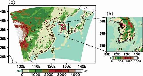
Figure 1 shows the simulation domain, and the model is run at a 15 km horizontal resolution. The domain contains 27 vertical layers up to 50 hPa. The initial and boundary conditions (ICs and BCs) for meteorology are specified using the Met Office Unified Model (UM; Bellouin et al. 2011) analysis processed by the Korea Meteorological Administration (KMA). The chemical ICs and BCs are specified by the MOZART-4 (Emmons et al. 2010) global chemical reanalysis produced by the Goddard Earth Observation System 5 (GEOS-5) global model with the MOZART chemistry.

Figure 1. (a) The simulation domain in Northeast Asia by WRF-Chem (only shaded region) is shown with surface elevation (unit: meter). The model uses the Lambert Conformal map projection. (b) shows the validation domain over the Korean Peninsula. The black circles in the figures indicate the ground PM observation sites, and the magenta triangles the AERONET sites for ground AOD observations

2.3 Aerosol data assimilation

This study uses the Gridpoint Statistical Interpolation (GSI) data assimilation system version 3.5 developed by NOAA, National Aeronautics and Space Administration (NASA), and NCAR, and the source code is available in public. The Community Radiative Transfer Model (CRTM; Weng et al. 2005) in GSI supports the 14 aerosol species resolved in GOCART, which is the aerosol scheme of the forecast model in this study. The 3-dimensional variational (3D-VAR; Barker et al. 2003) method is used for the data assimilation algorithm, which considers both errors from the model and observations referenced to the cost function J(x),

(1) $J\left(x\right)=\frac{1}{2}\left[\begin{array}{c}{\left(x-x_b\right)}^T{B}^{-1}\left(x-x_b\right)+{\left(y-H\left(x\right)\right)}^T\\ R^{-1}\left(y-H\left(x\right)\right)\end{array}\right].$(1)

To find the optimal analysis, the cost function is minimized, where x is the true (analysis) value, x_b the model background, y the observation, and H the observation operator. B and R represent the background and observational error covariance matrix, respectively. The method to derive the minimum cost function is to find the value x, which makes the derivative of J(x) as zero. As the analytical solution needs to inverse large background error covariance matrix, an iteration method finds the analysis fields that minimize the cost function. In GSI, the cost function J(x) is transformed into two directional functions to converge to the solutions quickly. The innovation (i.e. y – H (x)) is distributed to the model prognostic variables according to the predetermined background error covariance matrix.

The model background and observational error covariances are estimated based on Liu et al. (2011). The model background error covariance is calculated by the National Meteorological Center (NMC; Parrish and Derber 1992) method using the forecast error covariance averaged over the differences between two short-range model forecasts with different initial times but verifying at the same time. In this study, the model error is defined as the difference between 24- and 12-h WRF-Chem forecasts, and the error covariance for the aerosol variables is obtained using the values integrated for a month (i.e. 1–31 May 2016). Observation error covariance is specified as follows. The GOCI AOD error is set differently over the ocean and the land as a function of the aerosol optical depth τ,

(2) $E_{OCN}=0.185\tau +0.037,$(2)

(3) $E_{LND}=0.137\tau +0.08,$(3)

where E_OCN and E_LND are the observation errors for the ocean and the land, respectively (Choi et al. 2018). Surface PM error (E) is the sum of the measurement (E_M) and the representative (E_R) errors as below

(4) $E_M=E_{Max}+\frac{E_{Min}}{100}$(4)

(5) $E_R=E_T\cdot E_M\cdot \sqrt{\frac{\mathrm{\Delta }x}{S_{LU}}}$(5)

(6) $E=\sqrt{E_M^2+E_R^2}$(6)

where E_Max = 1.5 μg m⁻³ and E_Min = 0.75 μg m⁻³ are the maximum and the minimum errors for PM concentration, respectively. E_T = 0.5 is a tunable parameter; Δx = 15 km is the horizontal resolution, and S_LU = 3 km is the length scale of the influence of observations. These parameters are the standard values from the GSI configuration, which are slightly modified from Pagowski and Grell (2012).

2.4 Data assimilation and forecast cycle

The aerosol data assimilation is conducted in a 6-h interval at every 00, 06, 12, and 18 UTCs, when all 16 aerosol species in GOCART are updated by combining 6-h WRF-Chem forecasts (i.e. the model background states) started from the previous analysis and new observations from GOCI AOD and surface PM concentrations. The updated aerosol analysis fields are the initial conditions for the next 6-h WRF-Chem forecasts and data assimilation. The concentrations of gaseous chemical species are updated continuously by the model with no observational constraint. Meteorological variables are simulated by the model for 24 hours until they are reinitialized by the UM analysis at 00 UTC each day. The GOCI data are assimilated only for 00 UTC and 06 UTC, as they are unavailable for 12 UTC and 18 UTC. The time window of GOCI is set as ±3 hours, in which the AOD values are averaged in time with equal weightings. Liu et al. (2011) also applied the same time window in assimilating the MODIS AOD. Note that the hourly AODs at 00, 01, 02, and 03 UTCs are used for the 00 UTC data assimilation, and the data at 03, 04, 05, 06, and 07 UTCs are used for the 06 UTC data assimilation, respectively, as the GOCI is available only for daytime from 00 UTC to 07 UTC. On the other hand, the assimilation processes in situ PM data at the exact time of 00, 06, 12, and 18 UTCs.

This study conducts three DA runs: DA1 assimilates the GOCI AOD only, DA2 does the surface PM observations (PM₁₀ and PM_2.5) only, and DA3 does both GOCI AOD and the surface PM observations. The NoDA run indicates a free WRF-Chem forecast run restarted from the end of the previous 24-h run for chemistry and aerosol fields. In NoDA, the meteorological conditions are updated at 00 UTC every day as in the DA runs. Therefore, the difference between NoDA and DA is the impact of aerosol data assimilation.

Aside from the data assimilation cycle, the forecast runs start every day at 00 UTC and integrate for 24 h during the entire KORUS-AQ period with different initial conditions for the aerosol variables. DA1 denotes the forecast runs initialized from the GOCI AOD assimilation, DA2 from the surface PM assimilation, and DA3 from the assimilation of both GOCI AOD and the surface PM. Initial and boundary conditions for meteorological fields are from the 6-hourly global UM forecast fields initialized at 00 UTC. Initial conditions for gaseous chemistry fields are restarted from the previous 24-h forecasts.

3. Results

3.1 Time-series analysis during KORUS-AQ

During the KORUS-AQ period, there was a high concentration episode due to the Asian Dust on 7 May, clearly shown in the observed PM₁₀ concentration averaged over South Korea (Figure 2a). The day of 7 May was officially recorded as the Asian Dust day. It was a typical springtime day with no rainfall in South Korea, with the daily maximum temperature ranging from 19°C to 23°C. The highest concentration in the figure is at 00 UTC on 7 May with a peak concentration of 200 μg m⁻³. There is another time of relatively high PM₁₀ concentration during 25 May–1 June. The ground PM₁₀ concentration maintains at a high level above 80 μg m⁻³ on average, and this is attributed not to the Asian Dust but the long-range transport of air pollutants from China (Choi et al., 2021). There is also a buildup period of PM₁₀ concentration during 11–23 May due to the accumulation of local air pollutants under the stagnant weather until washed out by rain on 24 May.

Figure 2. Time series of (a) PM₁₀, (b) PM_2.5, and (c) AOD averaged for South Korea from the observations (black) and the simulations by NoDA (gray), DA1 (blue), DA2 (green), and DA3 (red). The observations show the average of all 346 NAMIS stations in South Korea in (a), and 16 AERONET stations located in South Korea in (b). For the validation, the nearest grid values to the ground stations are averaged to represent the model values. The unit is μg m⁻³ for PM concentrations and dimensionless for AOD

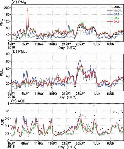
NoDA generally underestimates the observed values, particularly in those episodic events – the Asian Dust event, the local accumulation of air pollutants, and the long-range transport from China. Simulated temporal variation is also weaker than the observed. When the GOCI AOD is assimilated (DA1), the PM₁₀ analysis shows a much-reduced discrepancy from the observations, particularly for the three episodes. However, it is still likely to underestimate the values occasionally. When the surface PM data are assimilated (DA2), it delivers a better result. This is expected because the ground PM observations are directly provided for the data assimilation. When both satellite and ground observations are assimilated (DA3), the result is almost identical to DA2, showing the best fit for the observed time series. Especially in the Asian dust period on 7 May and the long-range transport regime of 25 May–1 June, it reproduces most of the observed PM₁₀ concentration.

The observed time series of PM_2.5 (Figure 2b) show a similar temporal variation as in the PM₁₀ time series, but also with some differences. Given that the PM₁₀ concentration includes PM_2.5, the surface PM_2.5 contributes relatively more to PM₁₀ in the long-range transport regime during 25 May–1 June. It suggests the natural dust, mostly sand, consists of large particles, whereas the anthropogenic emission contributes more to the PM_2.5 component. DA2 and DA3 experiments show almost identical results, and both reproduce the observed PM_2.5 concentration remarkably well. This is again due to the direct use of surface PM_2.5 observation in the data assimilation process, which tends to correct the systematic underestimation bias in NoDA as in the case of PM₁₀. However, DA1 shows more discrepancy from the observed values than DA2 or DA3. Unlike the case in PM₁₀, the satellite-only data assimilation tends to overestimate PM2.5 in those three major episodic events.

The observed AOD variation by AERONET stations (Figure 2c) shows a somewhat different time variation to PM₁₀ or PM_2.5. It does not show the highest values during the Asian dust event during 5–9 May. This implies that both variables do not always go along with each other. It suggests a weak coupling between the column-representing GOCI AOD and the surface-representing PM observations. Instead, the time series show sporadic increasing events in the late period of KORUS-AQ, for example, around 25 May–1 June and 7–11 June. The large temporal variation seems partly related to the statistical noise in the average with small data samples from the AERONET sites. The AOD values show much spread across the stations, especially after 25 May (not shown), indicating a large variability in AOD in space and time.

In the experiments, NoDA shows an underestimation of AOD as in the case of PM₁₀ or PM_2.5. The AOD simulated by DA2 shows an almost similar pattern to that by NoDA. The simulations by DA1 and DA3 are more consistent with each other, and both show a better consistency with the AERONET observations. However, they have difficulty in reproducing sporadic high concentration events, presumably due to the difference in spatial representativeness between ground and satellite AOD observations. When the two products are compared over the 21 AERONET sites, AERONET shows higher values than GOCI, although they maintain a high correlation (r = 0.76; See Supplementary Fig. S1).

3.2 Verification of major episodes

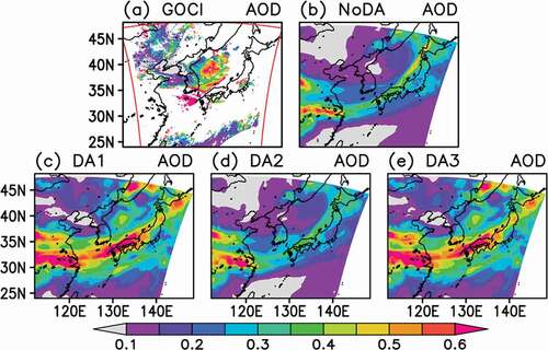
An example case of the Asian Dust event on 7 May 2016 during the KORUS-AQ period is selected to compare each data assimilation result (Figure 3). Although the GOCI observations show many missing values over the domain due to cloud contamination, they give a hint of the highly concentrated AOD plume across the southern part of the Korean Peninsula. It also shows the high AOD values in the East Sea. The NoDA run simulates the dust plume covering from China to South Korea and Japan (Figure 3b), suggesting that the WRF-Chem model driven by the observed meteorological conditions can simulate the dust event to some extent. However, the simulated AOD values are much weaker than the GOCI AOD. In South Korea, NoDA tends to simulate relatively high AOD values in the south but not as high as in the GOCI observations. Assimilation of AOD from the GOCI data only directly benefits the simulation results (DA1). It tends to increase the AOD values in most areas in the domain. Moreover, although the satellite AOD has a limitation in depicting the dust event clearly due to many missing values (Figure 3a), DA1 successfully identifies the large-scale dust event with considerably large AOD values (Figure 3c). Note that DA2 (Figure 3d) can only increase the AOD values in the land area of China. An AOD increase but in weak magnitude is also found in South Korea. The assimilation with the ground PM observations only shows that the dust plume becomes weaker over the oceans and in Japan, where no ground observations are available. This suggests a significant beneficial impact of using satellite AOD values in the aerosol data assimilation that fills the gap of ground observations. When both GOCI AOD and ground PM observations are assimilated altogether (DA3; Figure 3e), the result is consistent with DA1 with no significant difference.

Figure 3. The AOD distribution at 00 UTC on 7 May 2016 over Northeast Asia from (a) the GOCI observations, (b) NoDA (with no assimilated observations), (c) DA1 (the assimilation of GOCI only), (d) DA2 (ground PM only), and (e) DA3 (GOCI and ground PM). The area within the red frame in (a) indicates the spatial coverage by the GOCI instrument. The unit of AOD is dimensionless

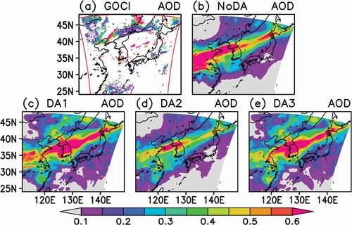
Figure 4 shows another example of a high-concentration event in South Korea due to long-range transport from China. In the GOCI observations (Figure 4a), AOD indicates high values from west to east at the 35° N latitude belt, although clouds contaminate most satellite pixels. NoDA (Figure 4b) simulates the high AOD plume stretching from central China to the middle part of the Korean Peninsula and the Hokkaido in Japan. However, the transport path tends to shift to the north so that the AOD values in South Korea become weak. When the satellite data are assimilated in DA1 (Figure 4c) and DA3 (Figure 4e), they tend to increase the magnitude of the AOD plume and expand it meridionally, covering most of South Korea with high AOD values. The data assimilation with surface PM observations only (Figure 4d) does not improve much from NoDA in magnitude and spatial pattern. The satellite data assimilation helps improve the values in the ocean points and the downstream side in northern Japan. Note that the surface PM assimilation further reduces the AOD values in central China from DA1 to DA3, where the satellite AOD has much uncertainty due to many missing values.

Figure 4. Same as in Figure 3 except at 00 UTC on 26 May 2016

3.3 Time-mean analysis patterns

Figure 5 compares the time-averaged surface PM₁₀ from the surface observation sites and the various data assimilation experiments. The observation (Figure 5a) shows high values in northern China, particularly over the Beijing-Tianjin-Hebei (BTH) area known for highly polluting coal-fired energy and manufacturing industries, transportation, and agricultural sectors. Another polluted region is located in the Yangtze River Delta centered in Shanghai. The surface PM concentration is maintained relatively lower in South Korea.

Figure 5. Time-averaged surface PM₁₀ concentration (unit: μg m⁻³) over Northeast Asia during KORUS-AQ from (a) surface observations, (b) NoDA, (c) DA1, (d) DA2, and (e) DA3 experiments. From (f) to (h), the figures show the differences for DA1, DA2, and DA3 from NoDA, respectively. The analysis fields at 00 and 06 UTCs are averaged

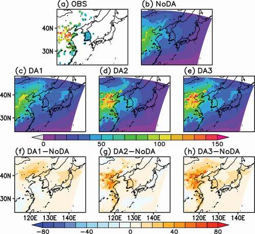
NoDA (Figure 5b) shows an overall underestimation of surface PM₁₀ for the BTH region in China and South Korea. The exception is in the continental interior in central China, where the model tends to overproduce the PM₁₀ concentration. Overall underestimation by NoDA is consistent with the findings from Figures 2–4, indicating a systematic model bias that can be generalized over the entire analysis period. The underestimation by the model can be caused by many factors, including surface emission, secondary formation, transport, and deposition process. It requires a more in-depth analysis and model experiments to pin down the root causes, which is well beyond the current research scope. This study just speculates that the model deficiency should be related to the considerable uncertainty in the surface-emission specified in the model and the parameterized aerosol chemistry and transport. The current emission inventory of the EDGAR-HTAP is produced by the bottom-up approach by integrating reported emissions, and possibly, there should exist many unknown sources or unreported emissions. Another deficiency is in the heterogeneous reactions associated with nitrogen and sulfur species. Many previous studies (e.g. Fairlie et al. 2010; Wang et al. 2012) indicate the significant contribution by the formation of nitrate and sulfate aerosols in East Asia to the total aerosol amount through heterogeneous thermodynamic reactions. The current MOZART and GOCART schemes do not explicitly represent these secondary aerosol formation processes. The model deficiency also lies in the parametrized natural dust scheme (See Section 2.2). The NoDA run underestimates the surface PM₁₀ concentration in northwest China, where the natural dust is originated from the Gobi Desert and transported to increase the aerosol amount. The WRF-Chem model used in this study enables the dust module in the GOCART scheme that lifts the natural dust dynamically by surface winds. The overall weak surface PM₁₀ concentration level in the northwest suggests a weak transport of natural dust from the source region by the model.

When only the GOCI AOD is assimilated (Figure 5c), surface PM₁₀ increases in most areas. In the difference from NoDA (Figure 5f), the AOD assimilation helps increase the surface PM₁₀ over the land area in northeastern China, North Korea, north of Japan, and the adjacent oceans. The results show more consistency with the surface observations over the BTH in China, where the positive contribution to the PM₁₀ concentration by the AOD assimilation is rather broad in space. In this regard, DA1 shows the difficulty in resolving local-scale sources in the major cities in the BTH region in China. In addition, DA1 slightly underestimates the ground concentration in South Korea.

When only the ground PM observations are assimilated (Figure 5d), DA2 now tends to resolve the local-scale sources in major cities over BTH by substantially increasing the PM₁₀ level comparing with NoDA. In addition, the surface data assimilation impacts are not limited to the observation data points but also in the adjacent regions. The data assimilation impact is most significant where the surface PM observations are available. Contrarily, its effect is almost negligible in North Korea and Japan, where no surface observation is provided (Figure 5g). Note that DA2 is almost identical to NoDA in the east of the Korean Peninsula, suggesting that the surface observations are limited in improving the analysis in farther regions. The surface PM₁₀ analysis is mostly benefited by assimilating both satellite and ground observation (Figure 5e). The difference from NoDA (Figure 5h) shows the features of simply adding two difference patterns of DA1 and DA2 from NoDA (Figure 5f and 5g).

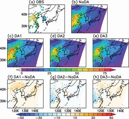
Different from the case of PM₁₀, the NoDA simulation for PM_2.5 (Figure 6b) shows much improvement over BTH in China with comparable magnitude to the observed values (Figure 6a). However, it still indicates regional discrepancy, such as the overestimation in the inland area in central China and the underestimation in the Yangtze River Delta and South Korea. The GOCI AOD only assimilation (Figure 6c) tends to increase the concentration from NoDA in most regions, particularly in northeastern China and northern Japan. The difference from NoDA (Figure 6f) is quite similar to the PM₁₀ case (Figure 5f). Contrarily, the surface PM data assimilation (Figure 6d and 6g) helps suppress the overestimation bias in the continental interior by NoDA. This is not driven by the satellite data assimilation (Figure 6f), as it is out of the GOCI retrieval domain. As in the case of PM₁₀, the surface data assimilation corrects NoDA near the observation sources (Figure 6g), while the satellite data cover a much wider region (Figure 6f). The difference from NoDA by DA3 (Figure 6h) is just close to the linear combination of those by DA1 and DA2 (Figure 5f and 5g), consistent with the case of PM₁₀.

Figure 6. Same as Figure 5 except PM_2.5.

Figure 7 compares the time-averaged spatial distribution of AOD from GOCI observations (Figure 7a), MERRA-2 (Figure 7b), the WRF-Chem simulations (Figure 7c), and the DA analyses (Figure 7d -f). In general, the time-averaged pattern by GOCI resolves highly polluted regions in the BTH and northeastern China, although the data are insufficient to locate other polluted areas in the south of BTH. The MERRA-2 shows the high AOD values in the comparison domain, with the maxima in BTH and central China. It also shows high values in Manchuria. The assimilation of GOCI AOD (Figure 7d) leads to the overall increase of the values from NoDA (Figure 7c). The maximum regions are also consistent with those in MERRA-2. The increment is considerably significant in northern China and Manchuria (Figure 7g). The overall increase in the AOD analysis fields demonstrates the benefit of satellite data assimilation, particularly in sparse observations such as in Manchuria and the regions where the surface observation is unavailable.

Figure 7. Time-averaged AOD over Northeast Asia during KORUS-AQ from (a) GOCI, (b) MERRA-2 reanalysis, (c) NoDA, (d) DA1, (e) DA2, and (f) DA3 experiments. From (g) to (i), the figures show the differences for DA1, DA2, and DA3 from NoDA, respectively. Areas with the available data less than 30% for the time average are eliminated in (a)

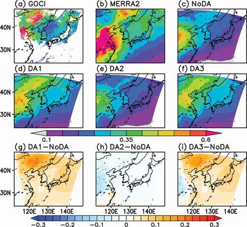
Note that the GEOS-5 producing MERRA-2 and the WRF-Chem in this study share the same GOCART aerosol scheme. Comparing MERRA-2 with DA1, we found that MERRA-2 shows much higher sulfate aerosols (not shown), suggesting significant differences in the anthropogenic emission between the analyses. However, one cannot exclude other factors, such as the differences in the assimilated observations (MODIS versus GOCI) and the chemical transport model (GEOS versus WRF-Chem).

The assimilation of surface PM observations (Figure 7e) tends to decrease the AOD values, particularly in China (Figure 7h), which is opposite to the case of the GOCI AOD assimilation (Figure 7g). It again suggests that the surface aerosol concentration may not represent well the aerosol concentration in the whole atmospheric column represented by AOD.

When both the satellite AOD and surface PM observations are provided to the data assimilation in DA3 (Figure 7f and 7i), the results are not much different from the case of DA1. This is somewhat expected because the direct assimilation of the AOD performs best for the AOD analysis. Comparing the AOD values in DA1 (Figure 7d), DA3 (Figure 7f) shows a slight decrease of the AOD values by the simultaneous assimilation of satellite data with the surface PM observations. It might suggest that the data assimilation performance is not always improved and often degraded by including additional observations. Our case implies the uncertain and non-linear relationship between AOD and surface PM values.

3.4 Impacts on forecast skills

Air quality forecasts can be improved by initializing the states of the forecast model with more realistic values consistent with the observations through the aerosol data assimilation technique. As the operational air quality forecasts for most countries are conducted for the ground PM concentration (Kukkonen et al. 2012; Marécal et al. 2015), this study compares the forecast skill for the PM concentration depending on each data assimilation experiment.

Before comparing the forecast skill by different initialization methods, this study first compares the quality of each analysis (i.e. the initial states of the forecasts) for PM₁₀, PM_2.5, and AOD, respectively, in the validation area in South Korea. Figure 8 shows the frequency scatter plots between observations and the model analysis from various experiments. This study compares the data assimilation performance quantitatively with two measures: the correlation between the observed and the analysis values and the relative root-mean-squared error (rRMSE) defined as the RMSE between the two divided by the time mean value of the observations.

Figure 8. Frequency scatter plots between observations (x-axis) and the model analysis (y-axis) for (a-d) PM₁₀, (e-h) PM_2.5, and (i-l) AOD. The model analysis in (a), (e), and (i) from NoDA, (b), (f), and (j) from DA1, (c), (g), and (k) from DA2, and (d), (h), and (l) from DA3. Frequency indicates the number of samples in each corresponding bin. The values at 00 and 06 UTC values are used for surface PM concentrations, 01 and 07 UTC values for AOD. The correlation (R) and the rRMSE (see the definition in the text) values are indicated in each panel

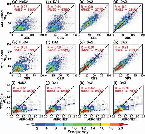
The comparison provides several insights into the aerosol data assimilation in this study. First, the model backgrounds (NoDA in Figure 8a, e and i) show difficulty in reproducing the observed values. All concentrations simulated without the data assimilation suffer from significant underestimations, particularly in PM₁₀. Considering more heterogeneity in the ground aerosol concentration and contributed by more aerosol species, PM₁₀ seems to show larger errors, comparing with other variables. Second, the data assimilations provide more accurate analyses of the observed values comparing with the model backgrounds. The overall low estimation biases are improved, and the scatter plots exhibit better alignment in the diagonal line. The data assimilation of surface PM observations fits the observed PM values best (e.g. Figure 8c, d, g and h)and the satellite AOD assimilation represents the best to the observed AOD values (Figure 8j and 8l). As the AOD validation is based on the independent AERONET data, the best correlation in AOD (r = 0.76) cannot be attained to such high values in PM₁₀ (r = 0.90) and PM_2.5 (r = 0.91). The AOD validation may also suffer from the difference in the spatial representativeness between satellite and ground-based AOD observations, as discussed in Figure 2. This improvement by the data assimilation may not be surprising because the data assimilation works properly in correcting biased model background states. However, note that the satellite AOD data assimilation results in improved surface PM analyses (Figure 8b and f), particularly in PM_2.5. A similar improvement can be found in the AOD analysis by assimilating surface PM observations (Figure 8k). This suggests the beneficial impacts of the 3D-VAR data assimilation methods. The observation data influences all of the model prognostic variables during the minimization of the cost function in Equation (1)(1) $J\left(x\right)=\frac{1}{2}\left[\begin{array}{c}{\left(x-x_b\right)}^T{B}^{-1}\left(x-x_b\right)+{\left(y-H\left(x\right)\right)}^T\\ R^{-1}\left(y-H\left(x\right)\right)\end{array}\right].$(1) . Finally, the data assimilation of both satellite AOD and ground PM observations does not necessarily improve individual data assimilation performance. Comparing the cases for PM₁₀ (cf Figure 8c and d), PM_2.5 (cf Figure 8g and h), and AOD (cf Figure 8j and l), the changes in the correlation and rRMSE seem to be negligible or even slightly degraded in terms of rRMSE. This suggests that the data assimilation with multivariate observations in this 3D-VAR algorithm may degrade the consistency with the original observations. However, it does not necessarily lead to the forecast skill degradation, as discussed in the next.

Figure 9 shows the forecast skill changes as the forecast lead time increases. In the figure, the forecast skill is measured by the temporal correlation between the observed and the forecast values as a function of forecast lead time. Another measure is the RMSE between the two. This study also conducted the statistical significance by the bootstrapping method.

Figure 9. The changes in the correlation of the surface (a) PM₁₀ and (b) PM_2.5 concentration forecasts and the RMSE for (c) PM₁₀ and (d) PM_2.5 from the initial state until +24 hr. The forecast skill is the average over all NAMIS stations in South Korea from the forecasts started at 00 UTC every day for 24 hours during KORUS-AQ. Each color line indicates the cases of NoDA (gray), DA1 (blue), DA2 (green), and DA3 (red). Shading indicates the 95% confidence level determined by the statistical significance test using the bootstrap method with 100,000 random samples for each experiment

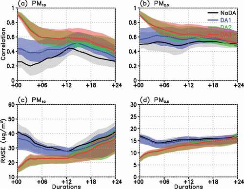
Generally, the correlation decreases, and the RMSE increases in time due to the systematic biases in the prediction. The forecast skill exhibits a considerable difference depending on the data assimilation method for initialization. The forecast runs started from the NoDA initial conditions show the most inferior performance among the experiments. In the PM₁₀ forecasts, the correlation starts even below 0.3 in the beginning, although there is a rebound of the skill in 12 hours from the initialized. The forecast skill remains less than 0.4, the minimum level for useful skill (Reichler and Roads 2005), during most of the forecast lead time. On the other hand, the RMSE tends to decrease in time until 12 h and starts to increase. This rebound of skill and the minimized error in about 12 h suggests the skill recovery due to the model’s capability to reproduce the observed diurnal variation of PM₁₀. The PM_2.5 forecasts by NoDA are better than those for PM₁₀, maintaining the skill around 0.5 throughout the forecast time. This is consistent with the results in Figure 8, where the data assimilation performs better for PM_2.5 and provides better initial conditions.

The results in Figure 9 further indicate that the air quality forecast skill is improved by the aerosol data assimilation using satellite and surface observations. Comparing with NoDA, any forecast started from the initial states produced by the data assimilation maintains a higher correlation throughout the forecast time. This indicates that the data assimilation impact, as represented by the correlation difference between DA forecasts and NoDA, tends to last at least 12 hours. When the initial conditions are determined by the data assimilation with both satellite AOD and surface PM observations (DA3), the forecast skill is the best for both surface PM₁₀ and PM_2.5. It maintains a correlation higher than 0.4 for all times. The RMSE is increasing as the forecast time increases as the initialization impact fades away. Comparing with DA3, DA2 performs comparable skills, which suggests that the data assimilation of surface PM data is the most important in improving the quality of the surface PM forecasts. Note that the forecast skill of DA3 overpasses the skill of DA2 in a few hours, for example in 12 hours for PM₁₀ and 6 hours for PM_2.5 after initialization. This implies that the simultaneous data assimilation with both satellite and surface data can maintain more balanced states among the variables and improve the forecast skill in an extended time.

When the satellite data is assimilated only (DA1), the correlation skill is overall increasing throughout the forecast time, with a slight decrease of RMSE. Comparing with DA2 and DA3, the relatively low forecast skills for the initial few hours are related to the less accurate calibration of surface PM concentrations by the assimilation of the satellite data only (see Figure 8b and f). It indicates that the satellite data also have limitations in representing the local variation of surface PM concentration.

4. Further discussion

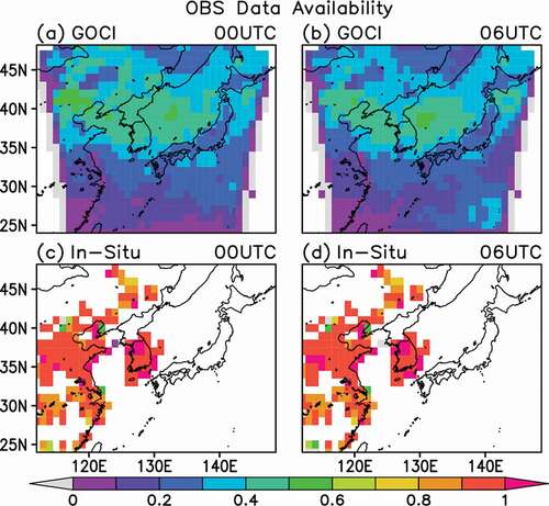
This study demonstrates the considerable benefits of using GOCI AOD in the data assimilation and forecasts and the limitations as well. The current data assimilation method in this study could have much room for further improvement. The first is to increase the AOD data availability for assimilation. Figure 10 compares the data availability of GOCI and surface PM observations at the time of data assimilation. The GOCI data covers a broader area (Figure 10a and b) comparing with the ground data (Figure 10c and d, although the availability is much less than 70% in most regions. Contrarily, the surface data show much higher availability reaching up to 100% in most areas, but the data are confined within the selected land area. The GOCI data are less available in the upstream region in central China and the south of 35° N, mainly due to clouds, although it provides the data at the Yellow Sea and North Korea, and northwest China, where the surface observations are unavailable. Therefore, our result with the GOCI data assimilation is limited by the data availability, and it has more potential to improve. Using the data assimilation of GOCI in all-sky conditions (Park et al. 2020) is expected to improve the performance significantly in this sense.

Figure 10. The GOCI AOD data availability for data assimilation at (a) 00 UTC and (b) 06 UTC within ± 3 hour time window. (c) and (d) indicate the availability of ground PM observations. The data availability is defined as the number of available data for the total required time. The values are smoothed by averaging 100 km by 100 km grids

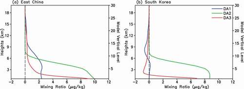
Another aspect is the discrepancy between the satellite AOD and the surface PM data. Figure 11 shows the vertical increment profiles of the total aerosol mixing ratio. Over China (Figure 11a), the satellite data assimilation tends to increase the aerosol concentration more aloft with a maximum at 3–6 km from the ground, while the increment by the surface PM assimilation is confined within the lowest 6 km above the ground. When both data are assimilated, the increment profiles correct not only the ground level but also in the mid- to upper-tropospheric levels. The results are qualitatively consistent with the findings in Schwartz et al. (2012). The benefit of using both satellite and in-situ observations is to adequately address the local emission-driven air pollution regime and the large-scale transport regime by steering winds in the free atmosphere. On the other hand, the increment profiles over South Korea (Figure 11b) show somewhat different features. The increment by the satellite AOD assimilation is relatively weak within the planetary boundary layer below 3 km altitudes and even negative in the middle troposphere. This suggests a difficulty in detecting local pollution contributions by the satellite AOD, and this discrepancy is worth further in-depth analysis. Downscaling the data by deep learning (Li et al. 2020) is expected to improve the locality of the satellite AOD.

Figure 11. Time-averaged vertical distributions of increments (analysis minus background) of the total aerosol mixing ratio (unit: ug kg-1) averaged over (a) East China (112–123 E, 30–41 N) and (b) South Korea (126–129 E, 34.3–37.8 N). DA1 (blue) is for the assimilation of GOCI only, DA2 (green) for the surface PM only, and DA3 (red) for both GOCI and surface PM assimilation

5. Summary and conclusions

This study develops an aerosol data assimilation system based on the WRF-Chem model that simultaneously assimilates the satellite-derived AOD and surface PM₁₀ and PM_2.5 observations. The assimilation and forecast skill is evaluated for the KORUS-AQ period (1 May to 10 June 2016) by integrating the analysis and forecast system at 15 km horizontal resolution.

When the verification is conducted in South Korea based on time series, the model background (NoDA) tends to underestimate the observed PM concentrations and AOD, presumably due to the deficiencies in emission and parameterized aerosol chemistry and transport processes by the model. While the data assimilation of surface PM in DA2 directly corrects the errors in the model backgrounds and describes the observed surface PM concentration level realistically, the improvement by the satellite AOD assimilation in DA1 is not trivial in representing surface PM concentration. When both satellite and surface observations are assimilated in DA3, the results show the best fit to the observed time series of the surface PM concentrations for the entire period of KORUS-AQ, which highlights the beneficial impacts of utilizing multiple observations.

Due to the broad coverage of satellite, the GOCI AOD assimilation also provides improved spatial representation of high concentration episodes in South Korea. While the improvement is limited to the land area of China and the Yellow Sea by the surface PM assimilation, the GOCI data assimilation shows significant beneficial impacts in representing large-scale aerosol transport plumes, including the regions of unavailable surface observations.

The data assimilation of GOCI AOD and surface PM observations provides the best analysis in surface PM concentrations in Northeast Asia, but with different aspects of the improvement. The GOCI AOD assimilation helps increase the aerosol amount in most of the domains, consistent with the surface observations and the pattern obtained from the independent MERRA-2 analysis. However, its impacts are rather broad in space showing difficulty in reproducing high surface PM concentration levels in the BTH area of northern China. In addition, the assimilation with GOCI AOD only tends to underestimate the surface PM concentration, particularly PM_10, in South Korea. This suggests an intrinsic difficulty in detecting the heterogeneous spatial distribution of surface PM by satellite data. In this regard, the combination of satellite and surface observations represents the best in resolving both broad and local pollution sources.

The data assimilation method produces substantial differences in the air quality forecast skill. Compared with the NoDA initialization, the air quality forecast skill is improved by any data assimilation method, with its impact lasting at least 12 hours or longer. When both satellite AOD and surface PM observations are initialized from the observational data, the forecast skill is the best for surface PM forecasts, maintaining a valuable level of the correlation skill higher than 0.4 for 24 hours.

The improvement of forecast skill by the GOCI AOD only assimilation is less than those expected by the surface PM data assimilation, as it exhibits less accurate calibration of surface PM concentration in the initial states. Nonetheless, it may still demonstrate the potential benefits of satellite data assimilation in improving the forecast skill in the data-sparse areas of surface PM observations. This study indicates two aspects of using GOCI AOD or any other satellite data to enhance aerosol data assimilation and forecast performance in Northeast Asia. First is the relatively low data availability comparing with the surface observations, primarily due to cloud contamination. The use of multiple satellites such as geostationary and polar-orbiting ones may increase the data samples and the quality of assimilation. A recent approach that used the machine learning algorithm to combine satellite information and the chemical transport model to fill the data gap would significantly improve the performance (Park et al. 2020). Another aspect is how to utilize the satellite AOD that represents the column-integrated information to the problem of air quality forecasts at the surface level. As shown in this study, two variables do not necessarily go along in the magnitude and temporal variations. One idea is to transform the satellite AOD into the surface PM variables based on the machine learning algorithms (Wang et al. 2010; Shin et al. 2020), which may reduce the uncertainty in the AOD observation operator in the radiative transfer model and improve the quality of the aerosol data assimilation at the surface by satellite data. This idea is now under test using the identical data assimilation and forecast framework used in this study.

Acknowledgements

The model simulations were performed by using the supercomputing resource of the Korea Meteorological Administration (National Center for Meteorological Supercomputer).

Data availability statement

The data that support the findings of this study are openly available in figshare at http://doi.org/10.6084/m9.figshare.14602458.

Disclosure statement

No potential conflict of interest was reported by the author(s).

Supplementary material

Supplemental data for this article can be accessed here.

Additional information

Funding

This study was supported by the Basic Science Research Program of the National Research Foundation of Korea (NRF), funded by the Ministry of Education, Science and Technology (NRF-2021R1A2C1008210)Ministry of Education [NRF-2021R1A2C1008210];

References

- Alfaro-Contreras, R., J. Zhang, J. S. Reid, and C. Sundar. 2017. “A Study of 15-year Aerosol Optical Thickness and Direct Shortwave Aerosol Radiative Effect Trends Using MODIS, MISR, CALIOP and CERES.” Atmospheric Chemistry and Physics 17 (22): 13849–13868. doi:https://doi.org/10.5194/acp-17-13849-2017.
- Al-Saadi, J., G. Carmichael, J. Crawford, L. Emmons, and S. Kim. 2016. “NASA Contributions to KORUS-AQ: An International Cooperative Air Quality Field Study in Korea.” Accessed 15 May 2021. https://goo.gl/VhssdX
- Althuwaynee, O., A. Balogun, and W. Madhoun. 2020. “Air Pollution Hazard Assessment Using Decision Tree Algorithms and Bivariate Probability Cluster Polar Function: Evaluating Inter-correlation Clusters of PM10 and Other Air Pollutants.” GIScience and Remote Sensing 57 (2): 207–226. doi:https://doi.org/10.1080/15481603.2020.1712064.
- Barker, D., W. Huang, Y. R. Guo, and A. Bourgeois. 2003. “A Three-dimensional Variational (3DVAR) Data Assimilation System for Use with MM5.” NCAR Tech Note 68.
- Bellouin, N., W. Collins, I. Culverwell, P. Halloran, S. Hardiman, T. Hinton, C. Jones, R. McDonald, A. McLaren, and F. O’Connor. 2011. “The HadGEM2 Family of Met Office Unified Model Climate Configurations.” Geoscientific Model Development 4 (3): 723–757. doi:https://doi.org/10.5194/gmd-4-723-2011.
- Brasseur, G., D. Hauglustaine, S. Walters, P. Rasch, J. F. Müller, C. Granier, and X. Tie. 1998. “MOZART, a Global Chemical Transport Model for Ozone and Related Chemical Tracers: 1. Model Description.” Journal of Geophysical Research: Atmospheres 103 (D21): 28265–28289. doi:https://doi.org/10.1029/98JD02397.
- Chen, F., K. Mitchell, J. Schaake, Y. Xue, H. L. Pan, V. Koren, Q. Y. Duan, M. Ek, and A. Betts. 1996. “Modeling of Land Surface Evaporation by Four Schemes and Comparison with FIFE Observations.” Journal of Geophysical Research: Atmospheres 101 (D3): 7251–7268. doi:https://doi.org/10.1029/95JD02165.
- Chin, M., P. Ginoux, S. Kinne, O. Torres, B. N. Holben, B. N. Duncan, R. V. Martin, J. A. Logan, A. Higurashi, and T. Nakajima. 2002. “Tropospheric Aerosol Optical Thickness from the GOCART Model and Comparisons with Satellite and Sun Photometer Measurements.” Journal of the Atmospheric Sciences 59 (3): 461–483. doi:https://doi.org/10.1175/1520-0469(2002)059<0461:TAOTFT>2.0.CO;2.
- Choi, M., J. Kim, J. Lee, M. Kim, Y. J. Park, B. Holben, T. F. Eck, Z. Li, and C. H. Song. 2018. “GOCI Yonsei Aerosol Retrieval Version 2 Products: An Improved Algorithm and Error Analysis with Uncertainty Estimation from 5-year Validation over East Asia.” Atmospheric Measurement Techniques 11 (1): 385–408. doi:https://doi.org/10.5194/amt-11-385-2018.
- Choi, Y., Y. S. Ghim, M. S. Rozenhaimer, J. Redemann, S. E. LeBlanc, C. J. Flynn, A. E. Perring, et al. 2021. “Temporal and spatial variations of aerosol optical properties over the Korean peninsula during KORUS-AQ.” Atmospheric Environment 254: 118301.
- Chou, M. D., M. J. Suarez, C. H. Ho, M. M. Yan, and K. T. Lee. 1998. “Parameterizations for Cloud Overlapping and Shortwave Single-scattering Properties for Use in General Circulation and Cloud Ensemble Models.” Journal of Climate 11 (2): 202–214. doi:https://doi.org/10.1175/1520-0442(1998)011<0202:PFCOAS>2.0.CO;2.
- Emmons, L. K., S. Walters, P. G. Hess, J. F. Lamarque, G. G. Pfister, D. Fillmore, C. Granier, A. Guenther, D. Kinnison, and T. Laepple. 2010. “Description and Evaluation of the Model for Ozone and Related Chemical Tracers, Version 4 (MOZART-4).” Geoscientific Model Development. European Geosciences Union 3 (1): 43–67. doi:https://doi.org/10.5194/gmd-3-43-2010.
- Fairlie, T. D., D. J. Jacob, J. E. Dibb, B. Alexander, M. A. Avery, A. van Donkelaar, and L. Zhang. 2010. “Impact of Mineral Dust on Nitrate, Sulfate, and Ozone in Transpacific Asian Pollution Plumes.” Atmospheric Chemistry and Physics 10 (8): 3999–4012. doi:https://doi.org/10.5194/acp-10-3999-2010.
- Fast, J. D., W. I. Gustafson, R. C. Easter, R. A. Zaveri, J. C. Barnard, E. G. Chapman, G. A. Grell, and S. E. Peckham. 2006. “Evolution of Ozone, Particulates, and Aerosol Direct Radiative Forcing in the Vicinity of Houston Using a Fully Coupled Meteorology‐chemistry‐aerosol Model.” Journal of Geophysical Research: Atmospheres 111 (D21): D21. doi:https://doi.org/10.1029/2005JD006721.
- Filonchyk, M., V. Hurynovich, H. Yan, and S. Yan. 2020. “Atmospheric Pollution Assessment near Potential Source of Natural Aerosols in the South Gobi Desert Region, China.” GIScience and Remote Sensing 57 (2): 227–244. doi:https://doi.org/10.1080/15481603.2020.1715591.
- Gelaro, R., W. McCarty, M. J. Suárez, R. Todling, A. Molod, L. Takacs, C. A. Randles et al. 2017. “The Modern-era Retrospective Analysis for Research and Applications, Version 2 (MERRA-2).” Journal of Climate 30 (14): 5419–5454. DOI:https://doi.org/10.1175/JCLI-D-16-0758.1.
- Gelaro, R., and Y. Zhu. 2009. “Examination of Observation Impacts Derived from Observing System Experiments (Oses) and Adjoint Models.” Tellus A: Dynamic Meteorology and Oceanography 61 (2): 179–193. doi:https://doi.org/10.1111/j.1600-0870.2008.00388.x.
- Giannadaki, D., J. Lelieveld, and A. Pozzer. 2017. “The Impact of Fine Particulate Outdoor Air Pollution to Premature Mortality.” Perspectives on Atmospheric Sciences, Springer, Cham: 1021–1026.
- Ginoux, P., M. Chin, I. Tegen, J. M. Prospero, B. Holben, O. Dubovik, and S. J. Lin, 2001. “Sources and distributions of dust aerosols simulated with the GOCART model.” Journal of Geophysical Research: Atmospheres 106 (D17): 20255–20273.
- Grell, G. A., and D. Dévényi. 2002. “A Generalized Approach to Parameterizing Convection Combining Ensemble and Data Assimilation Techniques.” Geophysical Research Letters 29 (14): 38. doi:https://doi.org/10.1029/2002GL015311.
- Grell, G. A., S. E. Peckham, R. Schmitz, S. A. McKeen, G. Frost, W. C. Skamarock, and B. Eder. 2005. “Fully Coupled “Online” Chemistry within the WRF Model.” Atmospheric Environment 39 (37): 6957–6975. doi:https://doi.org/10.1016/j.atmosenv.2005.04.027.
- Guenther, C., T. Karl, P. Harley, C. Wiedinmyer, P. I. Palmer, and C. Geron. 2016. “Estimates of Global Terrestrial Isoprene Emissions Using MEGAN (Model of Emissions of Gases and Aerosols from Nature).” Atmospheric Chemistry and Physics 6 (11): 3181–3210. doi:https://doi.org/10.5194/acp-6-3181-2006.
- Holben, B. N., T. F. Eck, L. Slutsker, D. Tanre, J. Buis, A. Setzer, E. Vermote, J. Reagan, Y. Kaufman, and T. Nakajima. 1998. “AERONET—A Federated Instrument Network and Data Archive for Aerosol Characterization.” Remote Sensing of Environment 66 (1): 1–16. doi:https://doi.org/10.1016/S0034-4257(98)00031-5.
- Hong, S. Y., and J. O. J. Lim. 2006. “The WRF Single-moment 6-class Microphysics Scheme (WSM6).” Asia-Pacific Journal of Atmospheric Sciences 42 (2): 129–151.
- Hong, S. Y., Y. Noh, and J. Dudhia. 2006. “A New Vertical Diffusion Package with an Explicit Treatment of Entrainment Processes.” Monthly Weather Review 134 (9): 2318–2341. doi:https://doi.org/10.1175/MWR3199.1.
- Janssens-Maenhout, G., F. Dentener, J. Van Aardenne, S. Monni, V. Pagliari, L. Orlandini, Z. Klimont, J. I. Kurokawa, H. Akimoto, and T. Ohara. 2012. “EDGAR-HTAP: A Harmonized Gridded Air Pollution Emission Dataset Based on National Inventories.” European Commission Publications Office, Ispra, Italy, EUR report No EUR 25229, 40.
- Justice, C. O., E. Vermote, J. R. Townshend, R. Defries, D. P. Roy, D. K. Hall, V. V. Salomonson, J. L. Privette, G. Riggs, and A. Strahler. 1998. “The Moderate Resolution Imaging Spectroradiometer (MODIS): Land Remote Sensing for Global Change Research.” IEEE Transactions on Geoscience and Remote Sensing 36 (4): 1228–1249. doi:https://doi.org/10.1109/36.701075.
- Kukkonen, J., T. Olsson, D. M. Schultz, A. Baklanov, T. Klein, A. I. Miranda, A. Monteiro et al. 2012. “A Review of Operational, Regional-scale, Chemical Weather Forecasting Models in Europe.” Atmospheric Chemistry and Physics 12 (1): 1–87.
- Lee, J., J. Kim, C. H. Song, J. H. Ryu, Y. H. Ahn, and C. Song. 2010. “Algorithm for Retrieval of Aerosol Optical Properties over the Ocean from the Geostationary Ocean Color Imager.” Remote Sensing of Environment 114 (5): 1077–1088. doi:https://doi.org/10.1016/j.rse.2009.12.021.
- Lee, P., J. McQueen, I. Stajner, J. Huang, L. Pan, D. Tong, H. Kim et al. 2017. “NAQFC Developmental Forecast Guidance for Fine Particulate Matter (PM2.5).” Weather and Forecasting 32 (1): 343–360. DOI:https://doi.org/10.1175/WAF-D-15-0163.1.
- Lee, T., S. B. Lim, Y. Sunwoo, J. H. Woo, B. Jung, and X. Zheng. 2008. “Design Issues of Reliable Data Transfer Mechanisms for Atmospheric Environment Monitoring.” Fourth International Conference on Networked Computing and Advanced Information Management, Seoul, Korea Vol. 1: 274–279.
- Li, L., M. Franklin, M. Girguis, F. Lurmann, J. Wu, N. Pavlovic, C. Breton, F. Gilliland, and R. Habre. 2020. “Spatiotemporal Imputation of MAIAC AOD Using Deep Learning with Downscaling.” Remote Sensing of Environment 237: 111584. doi:https://doi.org/10.1016/j.rse.2019.111584.
- Li, Z., Z. Zang, Q. Li, Y. Chao, D. Chen, Y. Ye, Y. Liu, and K. Liou. 2013. “A Three-dimensional Variational Data Assimilation System for Multiple Aerosol Species with WRF/Chem and an Application to PM 2.5 Prediction.” Atmospheric Chemistry and Physics 13 (8): 4265–4278. doi:https://doi.org/10.5194/acp-13-4265-2013.
- Liu, Z., Q. Liu, H. C. Lin, C. S. Schwartz, Y. H. Lee, and T. Wang. 2011. “Three‐dimensional Variational Assimilation of MODIS Aerosol Optical Depth: Implementation and Application to a Dust Storm over East Asia.” Journal of Geophysical Research: Atmospheres 116 (D23): D23. doi:https://doi.org/10.1029/2011JD016159.
- Marécal, V., V. H. Peuch, C. Andersson, S. Andersson, J. Arteta, M. Beekmann, A. Benedictow et al. 2015. “A Regional Air Quality Forecasting System over Europe: The MACC-II Daily Ensemble Production.” Geoscientific Model Development 8 (9): 2777–2813. DOI:https://doi.org/10.5194/gmd-8-2777-2015.
- Mlawer, E. J., S. J. Taubman, P. D. Brown, M. J. Iacono, and S. A. Clough. 1997. “Radiative Transfer for Inhomogeneous Atmospheres: RRTM, a Validated Correlated‐k Model for the Longwave.” Journal of Geophysical Research: Atmospheres 102 (D14): 16663–16682. doi:https://doi.org/10.1029/97JD00237.
- Pagowski, M., and G. A. Grell. 2012. “Experiments with the Assimilation of Fine Aerosols Using an Ensemble Kalman Filter. Journal of Geophysical Research.” Journal of Geophysical Research: Atmospheres 117 (D21): D21. doi:https://doi.org/10.1029/2012JD018333.
- Park, S., J. Lee, J. Im, C. K. Song, M. Choi, J. Kim, S. Lee et al. 2020. “Estimation of Spatially Continuous Daytime Particulate Matter Concentrations under All Sky Conditions through the Synergistic Use of Satellite-based AOD and Numerical Models”. Science of the Total Environment 713: 136516. doi:https://doi.org/10.1016/j.scitotenv.2020.136516.
- Parrish, D. F., and J. C. Derber. 1992. “The National Meteorological Center’s Spectral Statistical-interpolation Analysis System.” Monthly Weather Review 120 (8): 1747–1763. doi:https://doi.org/10.1175/1520-0493(1992)120<1747:TNMCSS>2.0.CO;2.
- Pope, C. A., III, R. T. Burnett, M. J. Thun, E. E. Calle, D. Krewski, K. Ito, and G. D. Thurston. 2002. “Lung Cancer, Cardiopulmonary Mortality, and Long-term Exposure to Fine Particulate Air Pollution.” Jama 287 (9): 1132–1141. doi:https://doi.org/10.1001/jama.287.9.1132.
- Randles, C. A., A. M. Da Silva, V. Buchard, P. R. Colarco, A. Darmenov, R. Govindaraju, A. Smirnov et al. 2017. “The MERRA-2 Aerosol Reanalysis, 1980 Onward. Part I: System Description and Data Assimilation Evaluation.” Journal of Climate 30 (17): 6823–6850. DOI:https://doi.org/10.1175/JCLI-D-16-0609.1.
- Reichler, T., and J. O. Roads. 2005. “Long-Range Predictability in the Tropics. Part II: 30–60-Day Variability.” Journal of Climate 18 (5): 634–650. doi:https://doi.org/10.1175/JCLI-3295.1.
- Saide, P. E., J. Kim, C. H. Song, M. Choi, Y. Cheng, and G. R. Carmichael. 2014. “Assimilation of Next Generation Geostationary Aerosol Optical Depth Retrievals to Improve Air Quality Simulations.” Geophysical Research Letters 41 (24): 9188–9196. doi:https://doi.org/10.1002/2014GL062089.
- Schwartz, C. S., Z. Liu, Y. Chen, and X. Y. Huang, 2012. “Impact of assimilating microwave radiances with a limited-area ensemble data assimilation system on forecasts of Typhoon Morakot.” Weather and forecasting 27 (2): 424–437.
- Seaton, A., D. Godden, W. MacNee, and K. Donaldson. 1995. “Particulate Air Pollution and Acute Health Effects.” The Lancet 345 (8943): 176–178. doi:https://doi.org/10.1016/S0140-6736(95)90173-6.
- Shin, M., Y. Kang, S. Park, J. Im, C. Yoo, and L. Quackenbush. 2020. “Estimating Ground-level Particulate Matter Concentrations Using Satellite-based Data: A Review.” GIScience and Remote Sensing 57 (2): 174–189. doi:https://doi.org/10.1080/15481603.2019.1703288.
- Unnithan, S., and L. Gnanappazham. 2020. “Spatiotemporal Mixed Effects Modeling for the Estimation of PM 2.5 From MODIS AOD over the Indian Subcontinent.” GIScience and Remote Sensing 57 (2): 159–173. doi:https://doi.org/10.1080/15481603.2020.1712101.
- Wang, X., W. Wang, L. Yang, X. Gao, W. Nie, Y. Yu, P. Xu, Y. Zhou, and Z. Wang. 2012. “The Secondary Formation of Inorganic Aerosols in the Droplet Mode through Heterogeneous Aqueous Reactions under Haze Conditions.” Atmospheric Environment 63: 68–76. doi:https://doi.org/10.1016/j.atmosenv.2012.09.029.
- Wang, Z., L. Chen, J. Tao, Y. Zhang, and L. Su. 2010. “Satellite-based Estimation of Regional Particulate Matter (PM) in Beijing Using vertical-and-RH Correcting Method.” Remote Sensing of Environment 114 (1): 50–63. doi:https://doi.org/10.1016/j.rse.2009.08.009.
- Weng, F., Y. Han, P. van Delst, Q. Liu, and B. Yan. 2005. “JCSDA Community Radiative Transfer Model (CRTM).” Proc. 14th Int. ATOVS Study Conf, Beijing, China: 217–222.
- Wiedinmyer, C., S. Akagi, R. J. Yokelson, L. Emmons, J. Al-Saadi, J. Orlando, and A. Soja. 2011. “The Fire INventory from NCAR (FINN): A High Resolution Global Model to Estimate the Emissions from Open Burning.” Geoscientific Model Development 4 (3): 625. doi:https://doi.org/10.5194/gmd-4-625-2011.