Intra-annual land cover mapping and dynamics analysis with dense satellite image time series: a spatiotemporal cube based spatiotemporal contextual method

ABSTRACT

Land covers provide essential information for understanding and detecting ecosystem, resources, and environmental dynamics. However, they are generally mapped at coarser temporal scales to study the inter-annual changes, while scant attention has been paid to map intra-annual land cover dynamics at finer temporal scales. Moreover, existing studies are still limited in intra-annual land cover mapping with dense satellite image time series (SITS). Accordingly, this study proposed a novel approach to accurately classify dense SITS for mapping intra-annual land cover dynamics. First, dense SITS is segmented at multiple spatiotemporal scales to generate optimal spatiotemporal cubes (ST-cubes), which are chosen as classification units. Second, the ST-cubes based on spectral, textural, spatial, and temporal features are integratively defined and employed in SITS classification. Third, the spatiotemporal context is modeled by a spatiotemporally extended conditional random field model that measures both spatiotemporal features and semantic correlation between geographic objects. Finally, the proposed method is applied to map the intra-annual land cover dynamics. Comparative experiments of SITS classification are carried out between our method and three existing competitors in a suburban area in Beijing, China, with a dense Sentinel-2 SITS. Moreover, based on the classification results, we analyzed the quantitative intra-annual dynamics of land cover. The result shows that our approach achieves significant improvements in classification accuracy over existing methods, indicating the effectiveness and superiority of the proposed method in mapping intra-annual land cover dynamics with dense SITS.

KEYWORDS:

• Land-cover mapping
• dense satellite image time series
• ST-cube-based image analysis
• spatiotemporal context
• intra-annual dynamics

1 Introduction

Land covers are physical and biological covers of the Earth’s surface, including water, vegetation, wetland, and human infrastructure, resulting from both natural and human forces (Running 2008; Houghton et al. 2012; Liu et al. 2020). It is fundamental to characterize the Earth’s ecological state and biophysical properties (Gómez, White, and Wulder 2016). However, the Earth’s land system is undergoing frequent and drastic changes due to natural and increasing anthropogenic activities, further affecting the climate, the earth’s surface attributes, and ecosystem services (Lambin et al. 2001; Reyers et al. 2009). Accordingly, more accurate, detailed, and timely information on land cover is highly desirable for better understanding the ecological and environmental variables on Earth.

Remote sensing has long been used for monitoring land cover and its changes over the past four decades due to its capability to observe land surface repetitively and consistently over large areas (Hansen et al. 2000; Jia et al. 2014a). Recent years have witnessed the development of satellite sensor technologies (MODIS, Landsat, and Sentinel series), improving both the spatial and temporal resolution (images can be weekly sensed at nearly 10 meters’ spatial resolution). Such satellite images continuously acquired for the same region in a period of time can form an image series, i.e. SITS (Guyet and Nicolas 2016). The growing availability of high-resolution SITS makes it possible to produce land-cover maps on a near real-time basis.

Many attempts have been performed to map land cover using multi-temporal images. Bi-temporal land cover mapping was commonly studied at the early stage (Petit, Scudder, and Lambin 2001; An and Brown 2008), which can capture abrupt changes in a given period. However, it is powerless in providing a comprehensive understanding of the successive land cover dynamics (Mena 2008). Therefore, other studies considered multi-temporal or SITS to map multi-year land cover and analyze its dynamics in long-term patterns. For instance, Wehmann and Liu (2015) utilized multi-temporal data to map land covers and detect their changes at roughly five-year intervals. Sexton et al. (2013) employed multi-year Landsat images to build a trajectory of land cover in the long-term schema. For all these works, however, the land cover type was considered constant within one year and mapped at relatively coarse temporal scales (usually in annual or 5-year intervals) to analyze the inter-annual abrupt or gradual changes, while the intra-annual dynamics such as seasonal vegetation change and biological migration were ignored. Concurrently, dynamics of land cover were studied through time series segmentation based on long-term time series data, such as BFAST (Verbesselt et al. 2010) and CCDC (Zhu and Woodcock 2014). They focused on obtaining land cover maps and their changes caused by disturbances, such as fire, deforestation, and phenological changes, where the intra-annual seasonal status and dynamics of land cover were not considered.

To obtain accurate intra-annual land cover maps to monitor areas with frequent intra-annual seasonal changes, temporally dense SITS data are considered. However, for classification with dense SITS, there are three critical issues. Firstly, existing works generally ignored the inherent spectral heterogeneity and multiscale properties of geographic objects in SITS’ spatiotemporal domains. Spatiotemporal heterogeneities of the spectrum will exist once the expression scale required by geographic objects are greater than spatiotemporal resolutions (Lopes et al. 2017; Blaschke et al. 2014), where geographic objects are composed of multiple pixels rather than a single pixel, enlarging the intra-class dissimilarity of features in spatiotemporal domain. However, previous SITS classification studies usually treated each pixel individually in the spatial domain and employed the spectral time series features of pixel to recognize geographic objects (Zhang et al. 2008; Peña and Brenning 2015). As a result, they cannot effectively resolve spatiotemporal heterogeneity. Additionally, geographic objects show various scales in spatial and temporal performance, where the spatial scale is reflected by the diversity in area and shape of their spatial domains, the temporal one is the various phenological changes driven by species diversity (such as the various phenological dynamics of different vegetation types). Accordingly, it is necessary to characterize geographic objects at multiple scales, which are ignored by previous studies in multi-temporal and SITS classification (Waldner, Canto, and Defourny 2015; Liu and Cai 2012). Previous studies delineate all geographic objects using a fixed scale, i.e. pixel scale, which has limitations in expressing the spatiotemporal distribution of geographic objects and cannot accurately classifying them.

Secondly, the spatiotemporal features contained in SITS have not been comprehensively utilized for classification. There is abundant information embraced in SITS especially for dense SITS with high spatial resolution, including spectral, spatial, and temporal items, aiding in discriminating different land covers (Xi and Du 2019). Nevertheless, existing works in SITS classification tend to consider only one aspect on either temporal or spatial features, resulting in unsatisfactory accuracy. For instance, Jia et al. (2014a) and Wang et al. (2015a) merely defined the spectral band, NDVI, and EVI time series based on pixels for classification, while ignoring spatial features, leading to substantial salt-and-pepper errors. Even some studies incorporated spatial features (Petitjean et al. 2012), they just focused on spatial enrichment of the pixel time series which was still limited in expressing the true spatial distribution of geographic objects. Moreover, the temporal change features were neglected, thus these methods are not suitable to map the intra-annual land cover with frequent temporal changes in dense SITS. Overall, integrative and accurate definition and employment of spatiotemporal features is still an issue in dense SITS classification.

Thirdly, existing studies are limited in modeling spatiotemporal correlations and contexts between geographic objects for SITS classification. Geographic objects in SITS exhibit correlations rather than randomness with each other in their spatial distribution and temporal variations, which can be described by spatiotemporal contexts (Xi et al. 2019). Two classic models, Markov Random Fields (MRF) and its improved one, i.e. Conditional Random Fields (CRF), have shown reliability in improving land cover classification of multi-temporal images (Benedek and Szirányi 2009; Jia et al. 2014b; Hoberg et al. 2014). However, for modeling spatiotemporal contexts in dense SITS and enhancing intra-annual land cover classification, existing studies have some limitations. First of all, previous studies (Wang et al. 2015b; Cai et al. 2014; Hoberg et al. 2014) generally modeled the spatiotemporal contexts based on pixel and its neighbors, which cannot accurately express spatiotemporal correlations between geographic objects. Since geographic objects often consist of multiple pixels (Blaschke et al. 2014), pixel-based contextual methods mostly modeled the intra-class similarity rather than the inter-class dependency between geographic objects. Therefore, a unit closer to geographic objects than a single pixel should be used as the basis for the spatiotemporal context model in SITS. Additionally, the feature and semantic dependencies between geographic objects were not comprehensively considered to model the spatiotemporal context in existing studies. Spatial contexts were usually calculated only based on the feature differences between spatial neighbors while the semantic factors were ignored (Liu and Cai 2012; Wehmann and Liu 2015). They specifically assigned the same classes to spatial neighbors for smoothing effects but discouraged the changes. Therefore, they are limited in expressing the semantic changes between spatial neighbors. For temporal context, likewise, most studies commonly modeled the temporal contexts as only the feature difference between temporal neighbors (Melgani and Serpico 2003; Wang et al. 2015a). Although some studies have considered the temporal semantic changes through the temporal transition probabilities of land cover (Liu and Cai 2012; Jia et al. 2014), they are devoted to the inter-annual abrupt changes with multi-temporal images while measuring the intra-annual seasonal changes with dense SITS is seldom considered. Moreover, existing spatiotemporal contexts studies were committed to enhancing the multi-temporal classification at a coarser temporal scale, hence their extension and application in dense SITS are still open.

In summary, existing works on temporal land cover mapping mainly focus on coarse temporal scales and are still limited in mapping intra-annual land cover with dense SITS. This study aims to propose a novel SITS classification method that can effectively address the aforementioned issues to accurately obtain frequent intra-annual land cover maps. A spatiotemporal model, ST-cube, is chosen as the basic unit for classification, which is proposed in our previous work (Xi et al. 2019) and has been proved to effectively reduce the spatiotemporal heterogeneities and better representing geographic objects at multiple scales in SITS compared to existing pixel and object units. Especially, in contrast to that previous work, which aims at resolving the multi-scale segmentation and generation of ST-cubes, this study focuses on the spatiotemporal feature extraction and classification based on ST-cubes. The contributions of this study are fourfold: (1) The spectral, textural, spatial, and temporal features are comprehensively defined and employed for classification based on ST-cubes to solve the problem of incomplete feature representation in existing studies. (2) Based on ST-cubes, a novel spatiotemporal extended CRF (ST-CRF) classification method is developed to model the spatiotemporal contexts between geographic objects. (3) The feature and semantic dependencies are integratively measured in both spatial and temporal contexts of ST-CRF to enhance dense SITS classification. (4) The proposed method improves the dynamic mapping accuracy of intra-annual land cover based on dense SITS.

2 Methodology

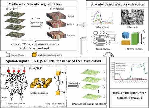
Aiming at generating frequent land cover maps with dense SITS and solving issues raised above, we propose a novel approach in this study, composed of four steps: (1) segmenting SITS to produce the optimal homogeneous ST-cubes; (2) ST-cube based features are defined and extracted based on the optimal segmentation results; (3) a spatiotemporal extended conditional random field (ST-CRF) classifier is proposed to classify dense SITS and produce the intra-annual land cover result; and (4) the intra-annual land cover dynamics are analyzed visually and quantitatively based on the land cover results (Figure 1).

Figure 1. The framework of our approach

2.1 ST-cube segmentation (ST-MRS) of SITS

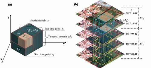
ST-cubes are selected as the basic classification units in SITS to effectively reduce the spatiotemporal heterogeneity and better express the spatiotemporal context between geographic objects. According to the definition, ST-cube is a collection of relatively similar pixels, which can be described as a homogeneous cubical area in SITS (Xi et al. 2019). Formulaically, considering a ST-cube organized as $C_i\left(S_i,\mathrm{\Delta }{T}_i\right)$, which includes information in spatial domain ($S_i$) and temporal domain ($\mathrm{\Delta }{T}_i$). $S_i$ characterizes the geographic position and shape of a ST-cube’s spatial domain, while $\mathrm{\Delta }{T}_i$ ($\mathrm{\Delta }{T}_i=⟨s_i,e_i⟩$) records the time interval of temporal domain (Figure 2a). ST-cube reflects the homogeneity and continuity of geographic object’s distribution in spatiotemporal domain and is suitable for establishing the spatiotemporal context between geographic objects. For instance, ST-cube $C_1$ reflects the homogeneous crop-growing state of a cropland with $S_1$ spatial area in $\mathrm{\Delta }{T}_1$ temporal interval (2017-09-12 to 2017-09-22, with a “yyyy-mm-dd” format, Figure 2b). In the adjacent temporal interval $\mathrm{\Delta }{T}_2$, $C_1$ is segmented into two spatially neighboring cubes $C_2$ and $C_3$, where $C_2$ and $C_3$ are temporally adjacent to $C_1$, reflecting the actual change that part of the $S_1$ cropland is harvested ($S_3$ area) and the remaining area remains a crop-growing state ($S_2$ area). Thus, the spatiotemporal contexts can be explicitly modeled by investigating the correlations between spatiotemporally neighboring cubes $C_1$, $C_2$, and $C_3$.

Figure 2. (a) The conceptual model of ST-cubes. (b) Specific expression examples of ST-cubes in SITS

ST-cube segmentation represents a fundamental step in ST-cube based SITS analysis, aiming at generating homogeneous ST-cubes with SITS. In this study, ST-cube segmentation is performed using the spatiotemporal multiresolution segmentation (ST-MRS) method developed in our previous work (Xi et al. 2019). Since the spatiotemporal scale parameters of ST-MRS control the spatiotemporal domain size of the ST-cubes, directly affecting the accuracy of SITS classification, thus the appropriate values for the spatiotemporal scale need to be determined first. In this study, the appropriate scales are determined by an iterative “trial-and-error” approach. We set up five gradually increased values for both spatial and temporal scales, which together formed 25 combinations of the final spatiotemporal scale parameters. Accordingly, 25 ST-cube segmentations are generated by ST-MRS and are evaluated by an unsupervised model, i.e. Spatiotemporal Global Score (STGS) (Xi et al. 2019), which measures the comprehensive goodness of heterogeneities within and between ST-cubes. In the end, the optimal segmentation scale of ST-MRS is determined as the one with the largest value of $STGS$, as it demonstrates the globally smallest heterogeneities within cubes and largest heterogeneities between cubes of ST-cube segmentations.

2.2 ST-cube based feature extraction

Based on the optimal ST-cube segmentation results, the ST-cube based features can be defined to describe ST-cube and serve for subsequent classification, including the spectral, textural, spatial, and temporal features. Spectral and textural features document geographic object’s physical radiation properties and can distinguish land cover with different reflectance properties. Spatial feature reflects distributions in size, shape, and geometries, while temporal one describes the characteristics of temporal dynamics in SITS. Based on the experience of existing image feature extraction and classification (Xi and Du 2019; Gómez, White, and Wulder 2016; Du, Zhang, and Zhang 2015), different spatiotemporal features can be used to distinguish different land cover types and should be integratively expressed and employed to obtain accurate land cover information in SITS. Therefore, considering the various land cover types in the study area, we choose a feature configuration of integratively expressing spectral, textural, spatial, and temporal features.

2.2.1 Spatiotemporal spectral features

Spatiotemporal spectral features of ST-cube can be decided based on the composition of material and appearance of the geographic object it represents, typical features include the mean, brightness, maximal difference ratio, and standard deviation of spectra of pixels within a ST-cube. The full-band spectra (i.e. Red, Green, Blue, Near-infrared, and Shortwave infrared) and two derived indexes, i.e. NDVI (normalized difference vegetation index) and EVI (enhanced vegetation index) are utilized to define these features. Thus, one defined feature usually corresponds to seven items. A total of 22 spectral features are extracted (Table 1).

Table 1. The definition of ST-features based on ST-cubes

Types	Names	Description	Ranges
Spectrum (22)	[Mean]	The average spectrum of a ST-cube	[m, M]
	[Brightness]	The weighted average spectrum of a ST-cube on each band	[m, M]
	[Max. diff.]	The ratio of the maximal difference between average spectrums on each band to brightness	[0, 1]
	[Std. dev]	Standard deviation of spectrum in a ST-cube	[0, 1]
	[NDVI]	Normalized difference vegetation index	[-1, 1]
	[EVI]	Enhanced vegetation index	[-1, 1]
Texture (125)	[Contrast]	The contrast derived from ST-GLCM	[0, 65,025]
	[Correlation]	The correlation derived from ST-GLCM	[0, 1]
	[Dissimilarity]	The homogeneity parameters derived from ST-GLCM	[0, 255]
	[Homogeneity]	The homogeneity derived from ST-GLCM	[0, 1]
	[Entropy]	The information entropy derived from ST-GLCM	[0, 10,404]
Spatial (9)	[Spatial area]	Area of the spatial domain polygon of a ST-cube	[0, N]
	[Border length]	Length of the inner and outer borders of the spatial domain of a ST-cube	[0, N]
	[Length/width]	Length-width ratio of the spatial domain polygon of a ST-cube	[0, ∞]
	[Rectangle fit]	Rectangular match degree of spatial domain polygon border	[0, 1]
	[Ellipse fit]	The goodness of the spatial domain polygon fitting into an ellipse	[0, 1]
	[Compactness]	Compactness of the spatial domain polygon	[0, ∞]
	[Radius ellipse]	Radiuses of maximal inscribed ellipse and minimal circumscribed ellipse	[0, ∞]
	[Shape index]	Smoothness of the spatial domain polygon border	[1, ∞]
	[Volume]	Size of the spatiotemporal domain of a ST-cube	[0, N]
Temporal (6)	[Start time]	Start time point of a ST-cube	[1, 365]
	[End time]	End time point of a ST-cube	[1, 365]
	[Time duration]	Length of the time duration of a ST-cube	[0, 365]
	[Middle time]	Middle time point of a ST-cube	[1, 365]
	[MaxDataT]	Time point of the maximum NDVI in a ST-cube	[-1, 1]
	[Amplitude]	Difference between maximum and minimum NDVI of a ST-cube	[-2, 2]

2.2.2 Spatiotemporal textural features

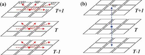
Geographic objects are various in the grays of different bands and distributions of pixels; this difference can be measured by textural features. Textures are the recurring local patterns occurring repeatedly in an image. Gray-level-co-occurrence matrix (GLCM) is one of the most effective methods for texture statistical analysis, which has been broadly used in mono-temporal texture calculation (Honeycutt and Plotnick 2008). In terms of SITS, since ST-cube describes the geographic object’s continuity and homogeneity in spatial and temporal domains, traditional GLCM can be extended to spatiotemporal-GLCM (ST-GLCM) to describe textures in both spatial and temporal dimensions. In spatial dimension, four symbiotic directions ($0^{\circ },{45}^{\circ },{90}^{\circ },\mathrm{a}\mathrm{n}\mathrm{d}{135}^{\circ }$) and one-pixel step length are selected in image spatial domain for each image layer in ST-cubes to generate GLCM (Figure 3a). Then, referring to existing experience (Du et al., 2015; Hoberg et al., 2014), five classic and conventional textural features (contrast, correlation, dissimilarity, homogeneity, and entropy) are derived from the GLCM. In the temporal dimension, the ${90}^{\circ }$ direction perpendicular to the spatial domain (i.e. parallel to the time axis) is taken as the symbiotic direction (Figure 3b) to generate GLCM at one-pixel step. Similarly, five textural features can be derived. Altogether, 125 spatiotemporal textural features are obtained at five bands (R, G, B, NIR, and SWIR) by integrating GLCM in spatial and temporal dimensions (Table 1).

Figure 3. Symbiotic structure of ST-GLCM: (a) The structure of spatial GLCM, where red lines indicate the four symbiotic directions. (b) The structure of temporal GLCM, where blue lines indicate the symbiotic direction

2.2.3 Spatial features

Spatial features of ST-cubes reflect the size, shape, and geometric distribution of geographic objects. Taking ST-cube as a whole, the spatial geometries of land cover can be specifically measured. Based on the geometric extraction of the spatial domain of ST-cube (Figure 1), we calculated the area and perimeter of the spatial domain. Additionally, how well the spatial domain can adapt to several typical shapes (e.g. squares, rounds, and ellipses) is of importance to distinguish different classes, including the shape index, rectangular fit, length-width ratio, and elliptic fit (Trimble 2011). Therefore, these spatial features of ST-cubes are also extracted (Table 1).

Temporal features related to ST-cubes can measure the temporal distribution, phenological stage, and temporal change characteristic of geographic objects, which helps discriminate temporally changed geographic objects. For example, the temporal distribution and change characteristics are distinguishable for different vegetation. At the ST-cube segmentation level, ST-cubes as wholes can also directly measure the temporal distribution of land cover. Based on ST-cube’s temporal domain information, referring to the definition of conventional phenological features (Jönsson and Eklundh 2004), we calculated the start and end times, time length, middle time point, and time amplitude of ST-cubes (Table 1). The amplitude refers to the differences between the largest and smallest NDVIs of ST-cubes.

2.3 Spatiotemporal CRF model (ST-CRF) for SITS classification

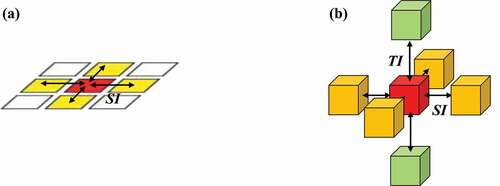
In this section, to consider the spatiotemporal context information, we construct a novel spatiotemporal CRF model based on ST-cubes by extending the traditional CRF to the spatiotemporal domain. For the traditional CRF usually employed in mono-temporal classification, only the interaction between spatial neighbors is considered (Figure 4a). In the SITS case, however, the correlation of both spatial and temporal neighbors should be considered (Figure 4b). The determination of spatiotemporal neighbors for ST-cubes refers to the neighboring rules in Xi et al. (2019).

Figure 4. The graph structure of (a): traditional mono-temporal CRF, where red square represents the to-be-processed pixel, yellow squares represent spatially neighboring pixels, i.e. SI the spatial interaction; and (b): ST-CRF in ST-cube based classification for SITS, red cubes represents the processed cube, yellow cubes represent spatial neighboring cubes, green cubes the temporal neighboring cubes and TI the temporal interaction

To clearly construct the ST-CRF model, the relative data items and symbols are defined at first. Considering an input SITS data organized in a ST-cube set $C=\left\{1,2,\dots ,N\right\}$ with a total number of N ST-cubes after ST-MRS segmentation. Therefore, all the ST-cubes can be expressed by feature set $Y=\left\{y_i\in {\mathbb{R}}^d|i=1,2,\dots ,N\right\}$, where $y_i$ is a d-dimensional spatiotemporal feature vector of the $i^{th}$ ST-cube in $C$. The labeled land-cover maps of SITS are represented as $X=\left\{x_1,x_2,\dots ,x_N\right\}$, where $x_i$’s value is taken from the label collection $L=\left\{1,2,\dots ,K\right\}$, with K denoting the number of total labels. The ST-CRF model thus can be defined as Eq. 1(1) $\begin{array}{r}P\left(X|Y\right)=\\ \frac{1}{Z}exp\left[\sum _{i\in C}A\left(x_i,Y\right)+\sum _{i\in C}\sum _{j\in S_i}SI\left(x_i,x_j,Y\right)+\sum _{i\in C}\sum _{k\in T_i}TI\left(x_i,x_k,Y\right)\right]\end{array}$(1) , which integrates the spatiotemporal feature cues, spatial and temporal contextual information. As a discriminative approach, the ST-CRF classification can be considered as finding the optimal label configuration $X$ by maximizing the posterior probability $P\left(X|Y\right)$.

(1) $\begin{array}{r}P\left(X|Y\right)=\\ \frac{1}{Z}exp\left[\sum _{i\in C}A\left(x_i,Y\right)+\sum _{i\in C}\sum _{j\in S_i}SI\left(x_i,x_j,Y\right)+\sum _{i\in C}\sum _{k\in T_i}TI\left(x_i,x_k,Y\right)\right]\end{array}$(1)

where $Z$ is a normalization constant called the partition function, $A$ represents feature association potential where the label $x_i$ of the $i$-th ST-cube is linked with the feature set $Y$. $SI$ is the spatial interaction potential and $TI$ is the temporal interaction potential. $S_i$ refers to the set of spatial neighboring cubes of the current ST-cube i; thus, $j\in S_i$ is a ST-cube that is a spatial neighbor of i. For TI, $T_i$ refers to the set of temporally neighboring ST-cubes of the $i$-th ST-cube, and $k\in T_i$ represents a temporal neighbor of i. The two terms $SI$ and $TI$ model the dependences of the class labels ($X$) and the spatiotemporal features ($Y$) between spatially and temporally neighboring cubes. The detailed descriptions of $SI$ and $TI$ are shown in the following sections.

2.3.1 Feature association potential

Feature association potential measures the correlation between semantic labels and the acquired SITS data, which calculates the cost of ST-cube i obtaining a specific label $x_i$, according to the spatiotemporal features. Accordingly, $A\left(x_i,Y\right)$ can be represented with a class membership probability that estimates the probability of $x_i$ obtaining a specific label with the given spatiotemporal feature vector. Generally, any discriminative classifier that has a probabilistic output can be utilized in this case. In this study, BP neural network (BPNN, Ding, Shu, and Yu 2011) is employed to generate the discriminative information of the semantic label based on features, due to its capability to deal with high-dimensional spatiotemporal features and complex nonlinear SITS classification problems. With this consideration, the$A\left(x_i,Y\right)$ can be defined as:

(2) $A\left(x_i,Y\right)=-ln\left(P\left[x_i=l|Y\right]\right)=-ln(P^{BPNN}\left[x_i=l|Y\right])$(2)

where $P^{BPNN}\left[x_i=l|Y\right]$ denotes the class membership probability of ST-cube $x_i$ with label l under BPNN. The used features ($Y$) in $A\left(x_i,Y\right)$ may vary from different cases; the features we adopted are the ST-cube based features given in Table 1.

2.3.2 Spatial interaction potential

The spatial interaction potential measures the spatial context between ST-cube and its spatial neighbors based on the semantic label factor and spatiotemporal feature factor. A widely accepted principle of spatial dependence is to assign the same labels to neighboring geographic objects, which can also be called spatial smoothing prior. However, neighboring geographic objects may have a class change if they actually correspond to different categories with different features. Therefore, to integrate the two spatial dependence principles, we employed an extension of the contrast-sensitive Potts model (Shotton et al., 2009) to represent the spatial interaction potential, which supports the spatial smoothing prior while also allows the semantic changes when the spatiotemporal features of spatially adjacent ST-cubes are distinctly different. Thus the $SI\left(x_i,x_j,Y\right)$ in Eq. (1)(1) $\begin{array}{r}P\left(X|Y\right)=\\ \frac{1}{Z}exp\left[\sum _{i\in C}A\left(x_i,Y\right)+\sum _{i\in C}\sum _{j\in S_i}SI\left(x_i,x_j,Y\right)+\sum _{i\in C}\sum _{k\in T_i}TI\left(x_i,x_k,Y\right)\right]\end{array}$(1) can be defined as Eq. (3)(3) $SI\left(x_i,x_j,Y\right)=\left\{\begin{array}{c}{\omega }_s\cdot \left\{1-exp\left(\frac{-{\theta }_s||f_{ij}\left(Y\right)|{|}^2}{R}\right)\right\},if{x}_i=x_j\\ {\omega }_s\cdot exp\left(\frac{-{\theta }_s||f_{ij}\left(Y\right)|{|}^2}{R}\right),if{x}_i\ne x_j.\end{array}\right.$(3) .

(3) $SI\left(x_i,x_j,Y\right)=\left\{\begin{array}{c}{\omega }_s\cdot \left\{1-exp\left(\frac{-{\theta }_s||f_{ij}\left(Y\right)|{|}^2}{R}\right)\right\},if{x}_i=x_j\\ {\omega }_s\cdot exp\left(\frac{-{\theta }_s||f_{ij}\left(Y\right)|{|}^2}{R}\right),if{x}_i\ne x_j.\end{array}\right.$(3)

In Eq. (3(3) $SI\left(x_i,x_j,Y\right)=\left\{\begin{array}{c}{\omega }_s\cdot \left\{1-exp\left(\frac{-{\theta }_s||f_{ij}\left(Y\right)|{|}^2}{R}\right)\right\},if{x}_i=x_j\\ {\omega }_s\cdot exp\left(\frac{-{\theta }_s||f_{ij}\left(Y\right)|{|}^2}{R}\right),if{x}_i\ne x_j.\end{array}\right.$(3) ), $\left||f_{ij}\left(Y\right)\right||$ denotes the Euclidean norm of $f_{ij}\left(Y\right)$, modeling the difference of spatiotemporal feature between two spatial neighbors; thus $\left||f_{ij}\left(Y\right)||=||y_i-y_j\right||$. ${\omega }_S$ is the weight for the impact of $SI$ in the whole classification procedure. ${\theta }_S$ is an interaction coefficient modulating the influence of feature-dependent items in $SI$. R refers to the number of dimensions of the spatiotemporal feature vector of ST-cube ($y_i$). For the spatial interaction potential, an identical influence of each feature dimension can be guaranteed with the division by R.

2.3.3 Temporal interaction potential

The temporal interaction potential models the dependency between each ST-cube and its temporal neighbors based on the classes and the spatiotemporal features. Actually, just like the $SI\left(x_i,x_j,Y\right)$, it can be constructed directly by penalizing the difference of feature vectors. However, this construction will be adversely affected by the additional data noise caused by the various imaging conditions (including atmospheric environment, illumination, climate, etc.) at different times, hindering the accurate expression of the temporal interaction potential. Moreover, the intra-annual changes of geographic objects usually show distinct trends, such as croplands are more likely to change from crop growing into crop harvested state due to harvesting activities rather than into built-up areas or water bodies. These trends can provide important guidance for land cover identification, hence it needs to be considered in the temporal interaction potential. Therefore, to integrate the temporal change trends of labels and feature dependency, we combine a category transition matrix and feature difference to construct the $TI\left(x_i,x_k,Y\right)$ model (Eq. 4)(4) $TI\left(x_i,x_k,\hspace{0.17em}Y\right)={\omega }_t\cdot \left(1-TM\left(x_i,x_k\right)\right)\cdot \left\{1-exp\left(-{\theta }_{t}D\left(x_i,x_k,\hspace{0.17em}Y\right)\right)\right\}$(4) .

(4) $TI\left(x_i,x_k,\hspace{0.17em}Y\right)={\omega }_t\cdot \left(1-TM\left(x_i,x_k\right)\right)\cdot \left\{1-exp\left(-{\theta }_{t}D\left(x_i,x_k,\hspace{0.17em}Y\right)\right)\right\}$(4)

In Eq. (4(4) $TI\left(x_i,x_k,\hspace{0.17em}Y\right)={\omega }_t\cdot \left(1-TM\left(x_i,x_k\right)\right)\cdot \left\{1-exp\left(-{\theta }_{t}D\left(x_i,x_k,\hspace{0.17em}Y\right)\right)\right\}$(4) ), ${\omega }_t$ weights the impact of $TI$ in the whole classification procedure. $TM$ refers to the temporal transition probability matrix that models the temporal change characteristics of land cover. The elements in $TM\left(x_i,x_k\right)$ relate to a conditional probabilities P$\left(x_i=l_i|x_k=l_k\right)$ of current ST-cube $i$ belonging to class $l_i$, where its temporal neighbor $k$ belongs to class $l_k$. According to the spatiotemporal neighboring rules (Xi et al., 2019), the times of temporal neighbors are chosen to consist of two adjacent previous and later time point $t_s-1$ and $t_e+1$ if they both exist, where $t_s$ and $t_e$ refer to the start and end times of the current ST-cube, respectively. $D$ denotes the feature difference between temporal neighbors as denoted by Eq. (5)(5) $D\left(x_i,x_k,Y\right)=\frac{\left|||y_i-y_k||-||\bar{y}\left(l_i\right)-\bar{y}\left(l_k\right)\right|||}{R}$(5) . ${\theta }_t$ is a tuning coefficient for the feature difference, making the tradeoff between the labels and feature dependency in $TI$.

(5) $D\left(x_i,x_k,Y\right)=\frac{\left|||y_i-y_k||-||\bar{y}\left(l_i\right)-\bar{y}\left(l_k\right)\right|||}{R}$(5)

where $\bar{y}\left(l_i\right)$ and $\bar{y}\left(l_k\right)$ represent the feature vector centers of the set of cubes with classes $l_i$ and $l_k$ in samples, specified by Eq. (6)(6) $\bar{y}\left(l_i\right)=\frac{{\sum }_{r\in S}I\left(x_r=l_i\right)\cdot y_r}{{\sum }_{r\in S}I\left(x_r=l_i\right)}$(6) and Eq. (7(7) $\bar{y}\left(l_i\right)=\frac{{\sum }_{r\in S}I\left(x_r=l_k\right)\cdot y_r}{{\sum }_{r\in S}I\left(x_r=l_k\right)}$(7) ), respectively. Therefore, $D$ penalizes the error in ST-cube’s temporal change $l_i\to l_k$ from class $l_i$ to $l_k$. If the category of the current cube is more different from $l_i$, which also means that the temporal change model is more different from $l_i\to l_k$, $D$ will get a larger value and vice versa.

(6) $\bar{y}\left(l_i\right)=\frac{{\sum }_{r\in S}I\left(x_r=l_i\right)\cdot y_r}{{\sum }_{r\in S}I\left(x_r=l_i\right)}$(6)

(7) $\bar{y}\left(l_i\right)=\frac{{\sum }_{r\in S}I\left(x_r=l_k\right)\cdot y_r}{{\sum }_{r\in S}I\left(x_r=l_k\right)}$(7)

In Eq. (6)(6) $\bar{y}\left(l_i\right)=\frac{{\sum }_{r\in S}I\left(x_r=l_i\right)\cdot y_r}{{\sum }_{r\in S}I\left(x_r=l_i\right)}$(6) and Eq. (7(7) $\bar{y}\left(l_i\right)=\frac{{\sum }_{r\in S}I\left(x_r=l_k\right)\cdot y_r}{{\sum }_{r\in S}I\left(x_r=l_k\right)}$(7) ), S is the sample set of ST-cubes, $I$ is an indicator function. Especially, to comprehensively measure differences of spatiotemporal features, the features used in $D\left(x_i,x_k,Y\right)$ are the same as those in $SI\left(x_i,x_j,Y\right)$ and $A\left(x_i,Y\right)$, including all features defined in Table 1.

2.3.4 Training and inference of ST-CRF

Accurate training and inference processes are critical for modeling the potential functions in ST-CRF. For training in this study, we only trained the parameters of $A\left(x_i,Y\right)$, including the number of network layers, the number of neurons in each layer, and the configuration parameters of network training (i.e. the goal error, maximum iteration epochs, and learning rate). Other model parameters such as those in $SI\left(x_i,x_j,Y\right)$and $TI\left(x_i,x_k,Y\right)$, including the weights ${\omega }_s$ and ${\omega }_t$, the tuning coefficients ${\theta }_s$ and ${\theta }_t$, and the elements in $TM\left(x_i,x_k\right)$, are set based on experimental experience (cf. Section 3.3).

Additionally, inference aims at predicting the optimal label configuration $X$ by globally taking the minimum value with the energy function. It is an NP-hard issue for the multiple classes classification of SITS. To find the optimal labeling of CRF, several inference methods have been developed recently, e.g. the iterated conditional mode (ICM), loopy belief propagation (LBP), and graph cut. For this study, we employed the graph-cut based on the α-expansion inference algorithm (Boykov, Veksler, and Zabih 2001), which is an efficient inference model for global energy minimization with multiple labels. Moreover, the graph-cut model has shown better results compared to the other two inference methods in a wide range of computer vision applications (Szeliski et al. 2008).

3 Experiments

3.1 Study area and used data collection

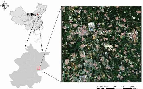
To verify the effectiveness of the proposed methods, a suburban area situated in Shunyi District in Beijing city (latitudes 40${ }^{\circ }$3ʹ 23.44” N to 40°12ʹ 4.49”N, and longitudes 116${ }^{\circ }$46ʹ 1.21” E to 116${ }^{\circ }$57ʹ 45.35” E) is chosen. The selected region covers 268 km² (Figure 5), containing typical land covers such as various crops, vegetation, and buildings, which show seasonal changes driven by annual temperature and climate interactions impacting plant phenology. The frequent temporal changes of land cover in this area allow the evaluation of the effectiveness of the proposed approach.

Figure 5. One image on 2017-08-06 of the Sentinel-2 SITS

The SITS data used in this study is composed of 42 Sentinel-2 images obtained at roughly 5 ~ 10 day intervals within one year from Feb 2017 to Feb 2018 (Table 2). These images were selected as there was as little cloud as possible in the study area, and the seasonal changes of land cover within one year can be mapped. Each image of the Sentinel-2 SITS consists of $1665\times 1610$ pixels and contains five spectral bands at a spatial resolution of 10 m. For all images, ortho-rectification and FLAASH atmospheric correction were conducted with ENVI 5.4 platform to reduce geometric and radiation errors, respectively.

Table 2. Information of the Sentinel-2 SITS. A “yyyy-mm-dd” format is used for the acquisition dates

Spatial Resolution	10 m
Spectral bands	B2 “Blue” (490 nm) B3 “Green” (560 nm) B4 “Red” (665 nm) B8 “Near-Infrared” (842 nm) B6 “Short Wave Infrared 1” (1610 nm)
Acquisition dates	2017-02-24, 2017-02-27, 2017-03-09, 2017-03-16, 2017-03-24, 2017-04-08, 2017-04-15, 2017-04-18, 2017-04-28, 2017-05-15, 2017-05-25, 2017-06-04, 2017-06-14, 2017-06-29, 2017-07-07, 2017-07-12, 2017-08-06, 2017-08-16, 2017-08-23, 2017-08-28, 2017-09-12, 2017-09-17, 2017-09-22, 2017-10-05, 2017-10-18, 2017-10-30, 2017-11-11, 2017-11-16, 2017-11-24, 2017-12-01, 2017-12-06, 2017-12-19, 2017-12-24, 2017-12-31, 2018-01-05, 2018-01-13, 2018-01-20, 2018-01-30, 2018-02-04, 2018-02-07, 2018-02-12, 2018-02-24.

3.2 Classification experiment setting

To verify the effectiveness of our method and produce accurate intra-annual land cover maps with dense SITS, we compare performances of our proposed ST-CRF and three existing popular methods: (i) the traditional no-contextual object-based classification (NOBC), (ii) the spatiotemporal contextual pixel-based classification (ST-PC), (iii) ST-cube based no-contextual classification (NSCC), and (iv) the proposed ST-cube-based spatiotemporal CRF classification (ST-CRF).

1. NOBC experiment. Object-based classification has been widely used in LU/LC classification of mono-temporal image (Blaschke 2010). In this experiment, Separate segmentation is conducted for each image of the SITS through Multiresolution segmentation (MRS) with eCognition platform to generate image objects, where a scale of 70 is utilized (ESP; Drǎguţ, Tiede, and Levick 2010). Object-based features including spectra, textures, and spatial geometries are defined and used for classification.

2. ST-PC experiment. The spatiotemporal context of pixels was considered and employed to improve the interpretation accuracy in many multi-temporal and SITS classifications (Hoberg et al. 2014; Wehmann and Liu 2015; Wang et al. 2015a). In this experiment, referring to the method in Wang et al. (2015a), we use a multi-temporal CRF to measure the spatiotemporal correlations of pixels. The full bands of spectra, two derived indexes, i.e. NDVI and EVI, and six phenological indicators of NDVI temporal profile (Jönsson and Eklundh 2004) are defined for ST-PC.

3. NSCC experiment. NSCC is proposed in our previous work (Xi et al. 2019) that took ST-cubes as basic units and classified SITS based on the optimal segmentation results and ST-cube based features without considering the context between cubes. Accordingly, ST-cube based features used in NSCC are the same as those defined in Section 2.2, including spectral, textural, spatial, and temporal features (Table 1).

4. ST-CRF experiment. Based on the optimal ST-cube segmentation result, the spatiotemporal contextual information between spatial and temporal neighbor ST-cubes was considered by the proposed ST-CRF model to enhance SITS classification (Section 2.3). The features used in ST-CRF include spectral, textural, spatial, and temporal features as defined in Table 1.

For effectively expressing the intra-annual change of land cover, based on the ground truth of the study area, we establish an eleven-class classification system (Table 3) that can fully embrace and reflect the intra-annual dynamics of land cover. The “Crop Growing,” “Crop Harvested,” and “Greenhouse Covering” are defined to demonstrate three major stages of the seasonal changes of cropland areas. The “Forest Leaf-on/off” and “Grass Leaf-on/off” corresponds to two main intra-annual phenological changes of vegetation coverages. The remaining four categories “Bareland,” “Built-up area,” “Road,” and “Water” are types that have no seasonal changes. Figure 6 illustrates the eleven typical images for each category of the classification system.

Figure 6. Typical images for eleven dynamic land cover classes

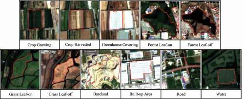
Table 3. The definition of the classification system

Code	Category	Definition
1	Crop Growing (CG)	Stage of cropland coverage with crop growing
2	Crop Harvested (CH)	Stage of cropland coverage after harvesting
3	Greenhouse Covering (GC)	Stage of cropland coverage with greenhouse covering
4	Forest Leaf-on (FN)	Leaf-on stage of forest coverage
5	Forest Leaf-off (FF)	Leaf-off stage of forest coverage
6	Grass Leaf-on (GN)	Leaf-on stage of grass coverage
7	Grass Leaf-off (GF)	Leaf-off stage of grass coverage
8	Bareland (BL)	Bare soil coverage without vegetation
9	Built-up Area (BA)	Construction coverage include buildings and impervious surface
10	Road (RO)	Road coverage includes urban roads and rural roads
11	Water (WA)	Water body coverage include rivers and lakes

To train and verify the proposed method, supervised samples of the eleven categories are selected based on pixels for each of the 42 images. The locations of sampled pixels in each image are randomly distributed with the proportions of their classes consistent with the practical ones. Table 4 gives the total number of all samples of the 42 images. For each class, the number of testing samples is about three times that of the training samples. Classes of samples are determined by visual interpretation based on high-resolution images from Google Earth, field survey photos, and expert field knowledge.

Table 4. The total number of samples of the eleven classes for all 42 images

Sample	Training (/pixels)	Testing (/pixels)
Crop Growing	2,020,672	6,240,518
Crop Harvested	3,917,863	11,665,184
Greenhouse Covering	48,652	151,275
Forest Leaf-on	225,758	711,265
Forest Leaf-off	253,031	789,093
Grass Leaf-on	57,705	171,571
Grass Leaf-off	81,062	268,416
Bareland	215,726	636,268
Built-up area	1,821,766	5,823,020
Road	148,523	451,353
Water	87,208	264,615

To evaluate the classification performance of the four methods, the classification results of the four methods at each time point were evaluated via visual observations and quantitative classification accuracy indicators. Four classic indicators including overall accuracy, per-class user’s, and producer’s accuracies are applied for assessment, which are calculated based on the typical confusion matrix model (Foody 2009). Additionally, the Z-score test is conducted to examine the statistical significance of the difference between classification results (Foody 2009; Thenkabail 2010).

3.3 Parameters setup of models

For the four methods, we selected a typical no-linear supervised classifier, i.e. BP neural network (BPNN), which has shown its superiority in handling non-linear SITS classification problems in the complex space-time domain (Ding, Su, and Yu 2011), to carry out the classification procedures. Especially, in ST-CRF, BPNN serves as the implementation of feature association potential with probabilistic output. As far as the parameters in BPNN are concerned, we established a 3-layer network, where the number of neurons in the hidden layer is set to 20, the goal error is 0.01, the maximum iteration epochs is 10,000 and the learning rate is 0.01. These parameters were determined for a tradeoff between accuracy and time efficiency based on a series of tests.

As for the parameters in spatial interaction potential of ST-CRF, the weighting factor ${\omega }_S$ and the interaction coefficient ${\theta }_S$ need to be determined. Based on the trial-and-error strategy and a series of cross-validation experiments, we set ${\omega }_S=0.8$ and ${\theta }_S=1.8$ as they correspond to a maximal training accuracy.

For the parameters associated with the temporal interaction potential of ST-CRF, the weight ${\omega }_t$, coefficient ${\theta }_t$ and the temporal transition matrix $TM$ need to be defined. Similarly, ${\omega }_t$ is set to 1.4 and ${\theta }_t$ set to 0.7 based on the cross-validation experiments. The weight ${\omega }_t$ is larger than the weight ${\omega }_S$ in spatial interaction potential because the temporal change and relation information between ST-cubes have a greater impact on the SITS classification results than the spatial ones. $TM$ describes the transition probability between temporal ST-cubes. Considering that determining the value of $TM$ through training requires a large number of training samples with the representative changes and training errors also may exist, the transition matrix $TM$ (Table 5) is set empirically based on the expert knowledge of the study area. The transition probabilities are given a large value in TM if the corresponding two land covers are more likely to change from the former to the latter one in the adjacent time. For example, the change from Crop Growing (CG) to Crop Harvested (CH) or Greenhouse Covering (GC), change from Forest Leaf-on (FN) to Forest Leaf-off (FF), and change from Grass Leaf-on (GN) to Grass Leaf-off (GF) are the major changes. The transition from cropland and vegetation to built-up area are penalized and correspond to smaller values, indicating the invariance of urban buildings and the seasonal variability of vegetation within one year.

Table 5. The parameters in temporal transition matrix $TM$, the vertical and horizontal items  represent the former and latter land covers in the adjacent time, respectively

	CG	CH	GC	FN	FF	GN	GF	BL	BA	RO	WA
CG	0.80	0.85	0.85	0.01	0.01	0.01	0.01	0.01	0.00	0.00	0.00
CH	0.85	0.80	0.20	0.01	0.01	0.01	0.01	0.01	0.00	0.00	0.00
GC	0.85	0.50	0.80	0.01	0.01	0.01	0.01	0.01	0.00	0.00	0.00
FN	0.01	0.01	0.01	0.80	0.85	0.05	0.05	0.05	0.00	0.00	0.00
FF	0.01	0.01	0.01	0.85	0.80	0.05	0.05	0.05	0.00	0.00	0.00
GN	0.01	0.01	0.01	0.05	0.05	0.80	0.85	0.05	0.00	0.00	0.00
GF	0.01	0.01	0.01	0.05	0.05	0.85	0.80	0.05	0.00	0.00	0.00
BL	0.01	0.01	0.01	0.05	0.05	0.05	0.05	0.80	0.05	0.05	0.01
BA	0.00	0.00	0.00	0.00	0.00	0.00	0.00	0.05	0.80	0.00	0.00
RO	0.00	0.00	0.00	0.00	0.00	0.00	0.00	0.05	0.00	0.80	0.00
WA	0.00	0.00	0.00	0.00	0.00	0.00	0.00	0.01	0.00	0.00	0.80

4 Results

4.1 Results of ST-MRS

As described in Section 2.1, 5 spatial scales (60, 80, 100, 120, 140) and 5 temporal scales (25, 45, 65, 85, 105) with gradient growth are employed, forming a total of 25 spatiotemporal scale parameter combinations (Table 6) to conduct the ST-cube segmentation. For all the 25 spatiotemporal scales, an equal weight (${\omega }_k$=1) is set to all the five bands; and the same weights, i.e. ${\omega }_{shape}$=0.1 and ${\omega }_{cpt}$=0.5 are also used.

Table 6. Characteristics of the 25 spatiotemporal scale combinations, where S_h is spatial scale, T_h refers to temporal scale, ${\omega }_k$ weight for each band, ${\omega }_{shape}$ and ${\omega }_{cpt}$ the shape and compactness weights in S_h.

Accordingly, a total of 25 ST-cube results are generated after being segmented by ST-MRS. The evaluation results by STGS of the 25 segmentations are given in Figure 7. The STGS achieved the largest value (STGS = 0.4907) at the spatiotemporal scale combination 100/65, indicating that for the segmentation perform with S_h = 100, T_h = 65, the resulting ST-cubes are, on average, most homogeneous internally and most different from their neighbors. Therefore, the scale (S_h = 100, T_h = 65) is selected as the optimum scale. A total of 78,837 ST-cubes are obtained at this scale and serve as the basic material for later ST-CRF classification.

Figure 7. The spatiotemporal global score (STGS) for all segmentations at 25 scales

4.2 Classification results of four experiments

Totally, $42\times 4$ land cover maps were generated using the four methods at 42 time points and their accuracies were evaluated at each time point. For the convenience of comparison and evaluation, specific results at four of all 42 time points (evenly distributed in one year), i.e. 2017-05-25, 2017-08-16, 2017-11-16, and 2018-02-12, were chosen and shown in Figure 8 for the four methods.

Figure 8. Classification results of the four methods at the chosen four time points

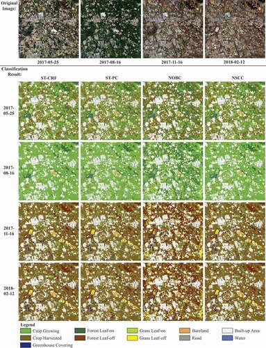
From the visual inspection of the classification results, ST-PC generates the salt-and-pepper noises in the results while the other three methods help to reduce these noises. Therefore, the results of ST-PC are more fragmented as it takes pixels as basic units and just models context based on pixels, thus the spatiotemporal heterogeneities of spectra have not been effectively resolved. The other three approaches, by contrast, are based on objects or ST-cubes which are more effective in considering and reducing spatiotemporal heterogeneities. As the results of NOBC are concerned, there are many misclassifications between vegetation types, such as errors between Crop Growing, Forest and Grass Leaf-on at 2017-05-25 and 2017-08-16, and errors between Crop Harvested, Forest and Grass Leaf-off at 2017-11-16 and 2018-02-12. This lies in that NOBC is unable to efficiently model the temporal contexts and features to distinguish different vegetation. NSCC greatly improves the salt-and-pepper noises and can correctly classify the vegetation types, illustrating the effectiveness of ST-cubes in reducing the spatiotemporal heterogeneities and expressing the spatiotemporal features. However, there are still some fragments in the results of NSCC; and misclassifications between Built-up Area and Greenhouse Covering also exist at 2017-11-16 and 2018-02-12 time points. Overall, ST-CRF produces the best result, as the fragments in NSCC are significantly smoothed and the misclassification errors of the other three methods are successfully eliminated, indicating the effectiveness of ST-cube and ST-CRF method in modeling the spatiotemporal contexts and enhancing the classification of dense SITS.

Tables 7 and 8 demonstrate the user’s, producer’s, and overall accuracies for each category and method of images in vegetation growing season (2017-08-16 time point) and out of growing season (2018-02-12 time point), respectively. ST-PC presents lower user’s and producer’s accuracies for categories with no temporal changes (i.e. Road, Built-up Area, and Water) than other methods in both time points due to the limitation of the pixel-based method in handling spectral heterogeneity. Conversely, NOBC provides the lowest accuracy for vegetation types (Crop Growing, Forest/Grass Leaf-on in 2017-08-16 and Crop Harvested, Greenhouse Covering, and Forest/Grass Leaf-off in 2018-02-12) but achieves higher accuracies in Road and Built-up Area than ST-PC, illustrating the significance of temporal features in time series image classification. In both vegetation growing and out of growing season time point, NSCC outperforms ST-PC and NOBC in terms of both producer’s and user’s accuracies of each category. ST-CRF outperforms the other three methods for all classes in the two accuracies and improves the overall accuracies by 2.67% (2017-08-16) and 3.23% (2018-02-12) than NSCC with the consideration of spatiotemporal contexts based on ST-cubes. Moreover, ST-CRF also achieves higher values than the other three methods in the average user’s and producer’s accuracies of all the 42 time points for each class, seeing the results in Tables 9 and 10. Overall, these results demonstrate that, in terms of SITS classification, ST-CRF can classify all categories more accurately than other approaches.

Table 7. Summary of quantitative accuracy evaluations of the four methods at vegetation growing season (2017-08-16). These shown in bold correspond to the highest value

Class	Method
	NOBC	ST-PC	NSCC	ST-CRF
User’s Accuracy (%)
Crop Growing	75.75	86.96	90.24	93.14
Forest Leaf-on	76.16	88.32	90.19	94.62
Grass Leaf-on	75.30	87.53	89.86	92.25
Bareland	86.68	85.87	91.28	92.82
Built-up area	87.29	84.22	90.67	94.18
Road	88.21	86.13	88.51	91.41
Water	95.67	94.08	95.83	96.36
Producer’s Accuracy (%)
Crop Growing	76.49	88.24	89.02	94.08
Forest Leaf-on	75.07	87.91	90.68	93.26
Grass Leaf-on	75.34	86.68	90.67	92.87
Bareland	87.31	86.62	91.35	93.76
Built-up area	88.77	83.65	91.48	93.69
Road	87.83	87.26	88.16	95.62
Water	94.36	93.84	95.27	97.15
Overall Accuracy (%)	83.73	87.71	90.85	93.52

Table 8. Summary of quantitative accuracy evaluations of the four methods at vegetation out of growing season (2018-02-12). These shown in bold correspond to the highest value

Class	Method
	NOBC	ST-PC	NSCC	ST-CRF
User’s Accuracy (%)
Crop Growing	85.89	86.53	91.17	93.87
Crop Harvested	74.63	88.24	89.94	92.95
Greenhouse Covering	79.34	88.48	87.98	93.14
Forest Leaf-off	74.24	87.63	90.26	93.73
Grass Leaf-off	75.58	87.75	90.78	94.28
Bareland	85.54	86.13	91.06	92.54
Built-up area	87.08	84.83	89.87	94.41
Road	88.16	87.02	89.03	92.17
Water	95.23	93.86	95.92	96.86
Producer’s Accuracy (%)
Crop Growing	86.05	87.25	90.98	93.25
Crop Harvested	73.61	87.86	89.79	93.83
Greenhouse Covering	79.66	88.73	88.46	94.06
Forest Leaf-off	75.86	88.09	90.51	92.57
Grass Leaf-off	75.34	88.11	91.14	93.65
Bareland	85.14	86.49	91.23	93.28
Built-up area	86.62	85.03	90.42	94.17
Road	86.95	86.24	87.95	94.92
Water	94.89	94.18	95.38	97.31
Overall Accuracy (%)	82.76	87.85	90.68	93.91

Table 9. Average user’s accuracy of all 42 time points for all four classifications. These shown in bold correspond to the highest value

Class	NOBC	ST-PC	NSCC	ST-CRF
Crop Growing	76.74	86.69	90.72	93.64
Crop Harvested	74.93	87.88	90.34	93.41
Greenhouse Covering	79.28	88.51	87.82	93.63
Forest Leaf-on	75.26	87.83	90.11	94.09
Forest Leaf-off	75.32	87.96	90.37	94.15
Grass Leaf-on	75.41	87.72	89.96	92.98
Grass Leaf-off	75.28	87.64	89.83	92.89
Bareland	86.13	85.96	91.15	92.93
Built-up area	87.16	84.58	90.23	94.38
Road	88.13	86.55	88.82	92.08
Water	95.38	93.81	95.84	96.65

Table 10. Average producer’s accuracy of all 42 time points for all four classifications. These shown in bold correspond to the highest value

Class	NOBC	ST-PC	NSCC	ST-CRF
Crop Growing	77.26	87.31	90.17	93.87
Crop Harvested	74.19	88.07	90.86	93.94
Greenhouse Covering	79.54	87.85	88.58	94.10
Forest Leaf-on	75.48	87.18	90.54	93.17
Forest Leaf-off	75.18	87.67	90.28	93.44
Grass Leaf-on	75.66	87.42	90.07	93.27
Grass Leaf-off	75.74	88.05	90.62	92.76
Bareland	86.36	86.18	91.31	92.97
Built-up area	87.68	84.32	90.52	94.08
Road	87.45	86.73	88.16	95.19
Water	94.67	94.04	95.31	97.22

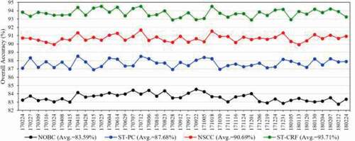
Figure 9 shows the overall accuracies of the classification results produced by the four methods for all 42 time points. The proposed ST-CRF achieves the best classification with the highest values in overall accuracy at each time point, as delineated by the green line. As far as the averages of the two indicators are concerned, the ST-CRF achieves the highest average accuracy at 93.71%, by an improvement of 3.02% over the no-contextual ST-cube based classification (NSCC), and 6.03% improvement over the pixel-based spatiotemporal contextual classification (ST-PC). These improvements prove the superiority of the proposed method in temporal-frequency finer SITS classification over the other methods.

Figure 9. Overall accuracies of results at all 42 time points. Values in parentheses of the legends are the average of the overall accuracy for all 42 time points

Table 11 presents the Kappa Z-score values between classification results of three combinations of methods, composed of ST-CRF and other three methods, at the chosen four time points (2017-05-25, 2017-08-16, 2017-11-16, and 2018-02-12). Z-score $>1.96$ or Z-score $<-1.96$ indicates that the difference between the two classification results is significant at the 5% significance level. From the comparison between ST-CRF and the other three methods, it is noticeable that the Z-score values of the three combinations are all larger than 1.96 at the four time points, indicating that the classifications generated by ST-CRF are significantly different from those generated by the other method and the proposed ST-CRF can significantly improve the land cover classification accuracy of SITS.

Table 11. Kappa Z-score values between classification results of two experiments at the chosen four time points. Underlined values indicate that results between the two methods are statistically significant ($p<0.05$)

Combination	2017-05-25	2017-08-16	2017-11-16	2018-02-12
ST-CRF vs NOBC	7.4671	7.2436	7.8195	7.5394
ST-CRF vs ST-PC	4.9217	4.8633	5.1637	4.8927
ST-CRF vs NSCC	3.2576	2.9485	3.0824	3.2318

The computational cost of the method is measured by the run time. For this study, experiments were performed on a personal computer with Intel Core i7-8565 U at a 1.80 GHz (1992 MH) CPU with 16.0-GB RAM. The features extraction, model training, and iteration inference of ST-CRF took around 11 min, 23 min, and 51 min, respectively, with a total time of about 85 min.

4.3 Intra-annual land cover dynamics analysis

After accurate classification of the dense Sentinel-2 SITS data by the proposed ST-CRF model, a total of 42 temporally frequent land cover maps, under a seasonally dynamic classification system (specified in Section 3.2), are generated to reveal the intra-annual dynamics of land cover in Beijing. Especially, for the convenience of demonstration and analysis, land cover maps at 12 of the 42 time points, that can completely reflect the land cover dynamics within one year, are selected and shown in Fig.10.

Figure 10. Intra-annual dynamic land cover maps classified by ST-CRF at 12 time points

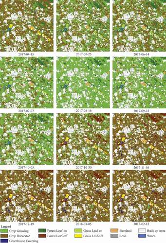
In the visual aspect, the crops of cropland started growing since April (2017-04-15), turning greener from April to August, and reaching the greenest on 2017-08-16. Of note is that the coverage of Crop Harvested increased from 2017-05-25 to 2017-06-14, as these increased areas were planted with winter wheat and were mostly harvested during this period. The harvested area of winter wheat would be planted with sorghum or soybeans in early July, as shown by areas that turn green from 2017-07-07 to 2018-08-16. Most crops began to be harvested from late September (2017-09-22) and reached the greatest in autumn and winter (2017-10-30 to 2018-02-12). The winter wheat was planted in November, demonstrated by the green area after 2017-11-16. Specifically, during winter (2017-11-16 to 2018-02-12), some cropland areas would be covered with white plastic greenhouses to protect crops as shown in the blue areas. Trees and grasses mostly withered since 2017-10-30, as shown by the leaf-off states of them.

Furthermore, the intra-annual dynamics of land cover can be studied from the quantitative aspect. Fig. 11 illustrates changes in land cover’s area at each time point, where Fig. 11a presents the changes of croplands coverage. Croplands change frequently between the state of Crop Growing and Crop Harvested within one year. The growth period of most crops was April (2017-04-08) to August (2017-08-16), as the area of Crop Growing increased from about 1830 hm² to 17,244 hm². Especially, croplands planted with winter wheat were harvested in June, marked by the increase in the height of the Crop Harvested column from 2017-05-25 to 2017-06-14. After 2017-08-28, other crops began to be harvested, and most of them were harvested in late September and October indicated by the sharp reduction in Crop Growing’s area and increase in Crop Harvested’s area from 2017-09-22 to 2017-10-30. The area of winter wheat was about 1050 hm², as shown by the black column after 171,116. Coverages of greenhouse gradually appeared in part of cropland areas since 2017-11-16, and in 2017-12-01, the greatest area of 294.38 hm² of croplands was covered with greenhouses. The entire coverage of croplands composed of these three fluctuated around 17,285 hm² illustrated by the total height of the three columns. Fig. 11b shows the change of forest and grass areas, most trees and grasses turned green in April (since 2017-04-08), and were under leaf-off condition since November (2017-10-30) till April in next year, according to the height changes of columns

Figure 11. Area changes of (a) croplands coverage and (b) forests and grasses coverage in the study area within 1 year

.

5 Discussion

5.1 Contribution of ST-cube and its related contexts for intra-annual land cover mapping

To investigate more real-time intra-annual dynamics at finer temporal scales (i.e. at monthly or weekly scale), detailed, accurate, and frequent intra-annual land cover maps are of great essence. This study proposed a ST-cube based contextual method (ST-CRF) and can effectively generate intra-annual land cover information with higher accuracy with dense SITS as it has three advantages.

First, ST-CRF takes ST-cubes as the basic units to delineate geographic objects more exactly, as spatiotemporal heterogeneities and scales in SITS can be well measured and expressed in ST-cubes. Spatiotemporal heterogeneities of spectrum will exist once the expression scale required by geographic objects is greater than spatiotemporal resolutions of time series data (Lopes et al. 2017). ST-cubes, as sets of similar pixels that show homogeneities in spatiotemporal properties based on the segmentation criteria of ST-MRS, can decrease the spectral heterogeneities inside cubes, confirmed by the improved accuracies of ST-PC by NSCC and ST-CRF in classification results (Fig. 9). The multi-scale characteristics require that multiple spatiotemporal scales should be adopted to represent and study geographic objects in SITS. In this study, 25 spatiotemporal scale combinations formed by five spatial and five temporal scales with gradient growth, are employed in ST-MRS to produce multiscale ST-cubes and determine the optimal segmentations for the ST-CRF classification.

Second, more comprehensive spatiotemporal features contained in SITS can be effectively expressed based on ST-cubes and utilized in ST-CRF classification. Prior works generally consider only one aspect on either temporal or spatial features (Jia et al. 2014a; Petitjean et al. 2012), resulting in unsatisfactory accuracy. By contrast, the spectral, textural, spatial, and temporal features are integratively defined and employed based on ST-cubes in this study (Section 2.2). The spectral and textural features document the physical radiation properties of geographic objects; the spatial ones embody the geometries and are crucial for classifying classes with high spatial heterogeneity, proved by the increased user’s and producer’s accuracies of NOBC, NSCC, and ST-CRF in Built-up Area and Road over ST-PC (Tables 9 and 10). Temporal features reflect the temporal and phenological changes and facilitate the distinction of classes with frequent changes, marked by the improvement of accuracies of ST-PC in vegetation types over NOBC. In general, the best results are obtained for each class with the comprehensive utilization of spectral, textural, spatial, and temporal features, as shown by the highest user’s and producer’s accuracies of ST-CRF for each class (Tables 9 and 10).

Third, spatiotemporal context information between geographic objects can be more accurately modeled with ST-CRF to enhance the intra-annual mapping of land cover with dense SITS. This innovation is attributed to the following reasons. First, the proposed ST-CRF measured the spatiotemporal contexts based on ST-cubes. This is different from prior works (Benedek and Szirányi 2009; Hoberg et al. 2014) that commonly measured the spatial and temporal dependencies based on pixel and its neighbors. Pixels have limitations in modeling the contexts between geographic objects as geographic objects often consist of multiple pixels spatially and temporally in SITS. The ST-cube is closer to the geographic object than the pixel, thereby can more accurately model the spatiotemporal contexts in SITS. Additionally, the spatiotemporal features and semantic contexts are integratively incorporated in ST-CRF, while previous contextual methods are usually formulated by only feature contexts between neighbors, which principally ignored the spatiotemporal semantic factors (Wang et al. 2015a; Wehmann and Liu 2015). In this study, an extended contrast-sensitive Potts is employed to represent the spatial interaction potential, calculating the dependencies of spatial neighbors based on both feature and semantic factors. Moreover, ST-CRF embraces the expert knowledge about temporal semantic changes of land cover in temporal interaction potential, which provides key guidance information for frequent intra-annual changes of land cover within dense SITS, hence improving the classification accuracy as shown in the results in Section 4.2.

5.2 Comparison of ST-CRF and the state-of-the-art methods

To verify the effectiveness and superiority of the proposed method, we compare the ST-CRF with three existing popular methods for SITS classification: (1) the traditional no-contextual object-based classification (NOBC), (2) the spatiotemporal contextual pixel-based classification (ST-PC), and (3) no-contextual ST-cube based classification (NSCC).

First, the NOBC is a classic approach in land cover mapping of mono-temporal images and has been proved to be more effective than the mono-temporal pixel method (Blaschke 2010). Generally, NOBC has two key components: one is the segmentation to generate objects and the other is the classification of image objects with features. Since it is committed to mono-temporal classification, for handling SITS classification, segmentation and classification should be conducted for each image of the STIS separately in NOBC, thus the temporal consistency and features cannot be effectively expressed and employed. Therefore, NOBC produces the lowest user’s and producer’s accuracies of vegetation types of land cover that perform frequent changes in SITS, as shown in Tables 9 and 10. Moreover, the lowest average overall accuracy at 83.59% is obtained by NOBC compared with the other three temporal methods (Fig. 9a), illustrating the inapplicability of NOBC to the classification of time-series images.

Second, the spatiotemporal contextual pixel-based classification is a popular approach and has been widely applied in existing multi-temporal and time series image land cover mapping (Wang et al. 2015a). Generally, ST-PC models the spatiotemporal contexts and correlation concerned with geographic objects based on pixels and their spatial and temporal neighbors (Wang et al. 2015a; Hoberg et al. 2014); thus it improves the accuracy over NOBC. Since pixels have limitations in resolving the spatial-spectral heterogeneities and expressing spatial geometry features, ST-PC achieves the lowest user’s and producer’s accuracies in categories with no temporal changes and high spatial heterogeneity (i.e. Road, Built-up Area, and Water) than the object- and cube- based methods (Tables 9 and 10). By using ST-cubes to express spatiotemporal contexts, ST-CRF increases the overall accuracy by a range of 4.70%~7.41% for results at all 42 time points compared to ST-PC, indicating the advancement of the proposed method in denes SITS classification.

Third, the no-contextual ST-cube based classification is a method proposed in our previous work for land cover mapping with SITS (Xi et al. 2019). NSCC takes ST-cubes as processing units, thus it requires segmentation of SITS by ST-MRS first to generate ST-cubes, and then classify SITS based on optimal segmentation of ST-cubes and ST-cube based features. Especially, NSCC differs from the proposed ST-CRF in that it does not consider the spatiotemporal contexts between cubes in SITS classification. Consequently, over NSCC, ST-CRF increased the average user’s and producer’s accuracies by about 3%~5% for most classes and can reach 7% in the producer’s accuracies of Road (Tables 9 and 10). Moreover, the average overall accuracy is increased by 3.02% by ST-CRF, illustrating the effectiveness of spatiotemporal contexts in enhancing the classification with dense SITS.

Overall, the comparison carried out in this study clearly shows the superiority of the proposed ST-CRF over the state-of-the-art methods in dense SITS classification for intra-annual land cover mapping.Fig. 11

5.3 Contribution of spatiotemporal features to SITS classification

In this study, we expressed and employed spectral, textural, spatial, and temporal features to conduct SITS classification. To understand how much do different spatiotemporal features contribute to the classification accuracy of different categories, feature contribution evaluation is carried out in this section. Especially, in ST-CRF, we employed BPNN to model the feature association potential, due to its stronger self-learning ability and better applicability for high-dimensional spatiotemporal features and complex nonlinear SITS classification problems than other traditional classifiers (such as SVM (Support Vector Machine) and RF (Random Forest)). However, BPNN cannot realize the evaluation of feature contribution degree, thus we adopt RF as feature association potential of ST-CRF, as it excels in effectively evaluating the feature contribution. The other configurations of ST-CRF remain unchanged (including features, parameters, and samples) to classify SITS and obtain feature contribution degrees.

Consequently, the contribution degree result is presented in Fig. 12. Especially, the contributions of spectral and textural features are counted together illustrated by the yellow column, as they both are expressions of the reflection properties of geographical objects. According to the result, spectral and textural features show similar contribution degrees (about 3%) in each category. As spectral and textural features are the characterization of the basic physical radiation and reflection properties of geographic objects, these two features are of equal importance to the interpretation of all kinds of land cover. Spatial characteristics show a higher contribution degree than spectral, textural, and temporal ones in the classification of built-up area, road, and water, as shown by the blue columns. Since roads, waters (rivers), and built-up areas often have distinct characteristics in spatial distribution and shape, e.g. the length-width ratio of roads and rivers is often much larger than other geographic objects, the spatial features show greater distinguishability and higher contribution for these types. Conversely, temporal features obtain higher contribution for classifying croplands (crop growing, crop harvested, and greenhouse covering), forest (forest leaf-on/off), and grassland (grass leaf-on/off), as demonstrated by the gray column. Croplands, forests, and grassland have frequent seasonal and phenological changes within one year. The ST-cube based temporal features can effectively describe the seasonal change distribution characteristics of these geographic objects, thus they show greater importance to distinguish land cover types with temporal changes.

Figure 12. Contribution degrees of spatiotemporal features for each category

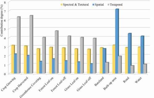
Accordingly, in SITS classification, spectral, textural, spatial, and temporal features are all useful and have distinct contributions and importance for classifying different land cover types. Therefore, it is suggested that spectral, textural, spatial, and temporal features should be comprehensively expressed and utilized to obtain an accurate classification of SITS.

5.4 Limitations

Despite the effectiveness of our method, several issues remain to be studied further. First, the optimal spatiotemporal segmentation scales in ST-MRS algorithm are manually determined through a “trial-and-error” approach, which is somewhat subjective and time-consuming; and the global optimal scale occasionally does not match well with the inherent scales of some geographic objects. Accordingly, some efficient automatically and self-adaptive scale chosen methods (e.g. Zhang and Du 2016) can be extended to SITS and utilized in future studies. Second, the parameters in the spatial interaction potential of ST-CRF are also determined by the trial-and-error strategy while the parameters in the transition matrix of temporal interaction potential are found empirically. Thus these parameters may not be appropriate for SITS classification in other areas with different change types. A more deterministic and automatic parameter selection method for ST-CRF needs to be applied in future studies. Third, as the iterative inference step of ST-CRF is time-demanding, further improvements should be made on optimizing its time efficiency. Forth, the proposed method is dedicated to frequently intra-annual land cover mapping of geographical areas, which is experimentally verified in one suburban area of Beijing and obtains satisfactory results. Thus, it should be applied to multiple areas to further ensure its generalization and spatial transferability, which will also be our future work.

6 Conclusions

In this study, a ST-cube based SITS classification approach (i.e. ST-CRF) that incorporates the spatiotemporal features extraction and context modeling is firstly proposed to map frequent intra-annual land cover dynamics with dense SITS. Experiments are conducted in Beijing, China with a dense SITS consists of 42 Sentinel-2 images to verify the effectiveness of our method. Consequently, the following conclusions can be drawn. First, ST-cube is more appropriate to delineate and extract geographic object in spatiotemporal domain with SITS than existing pixel and object units, as the spatiotemporal heterogeneity and scale characteristic can be effectively measured. Second, based on ST-cubes, the spectral, textural, spatial, and temporal features can be comprehensively and accurately defined and utilized for SITS classification. Third, the feature and semantic dependencies between geographic objects can be effectively expressed in the spatiotemporal contextual model of ST-MRS. Fourth, spatiotemporal context can significantly improve the accuracy of dense SITS classification. Fifth, the proposed ST-CRF outperforms existing popular temporal classification methods, and can produce more accurate intra-annual land cover maps with dense SITS.

To summarize, the proposed method contributes to intra-annual land cover mapping with dense SITS data, showing the potential in land cover dynamics research at a finer temporal scale.

Highlights

1. ST-cube based classification method is proposed to map intra-annual land cover.

2. Spatiotemporal features are comprehensively extracted based on ST-cubes.

3. Models the cube based spatiotemporal context to enhance dense SITS classification.

4. Improves intra-annual land cover mapping over three existing popular methods.

5. Demonstrates the potential in analyzing intra-annual land cover dynamics.

Acknowledgements

The work presented in this paper is supported by the National Natural Science Foundation of China (No. 41871372) and the Key Laboratory of Surveying and Mapping Science and Geospatial Information Technology of Ministry of Natural Resources [2020-2-1].

Data availability statement

The data used in this study are freely available as follows.

Sentinel-2 time series image data: https://scihub.copernicus.eu/dhus/#/home

The models and codes generated from this study are available upon request to the corresponding author.

Disclosure statement

No potential conflict of interest was reported by the author(s).

Additional information

Funding

This work is funded by the National Natural Science Foundation of China [41871372] and the Key Laboratory of Surveying and Mapping Science and Geospatial Information Technology of Ministry of Natural Resources [2020-2-1];Key Laboratory of Surveying and Mapping Science and Geospatial Information Technology of Ministry of Natural Resources (cn) [[2020-2-1]];

References

- An, L., and D. G. Brown. 2008. “Survival Analysis in Land Change Science: Integrating with GIScience to Address Temporal Complexities.” Annals of the Association of American Geographers 98 (2): 323–344. doi:https://doi.org/10.1080/00045600701879045.
- Benedek, C., and T. Szirányi. 2009. “Change Detection in Optical Aerial Images by a Multilayer Conditional Mixed Markov Model.” IEEE Transactions on Geoscience and Remote Sensing 47 (10): 3416–3430. doi:https://doi.org/10.1109/TGRS.2009.2022633.
- Blaschke, T. 2010. “Object Based Image Analysis for Remote Sensing.” ISPRS Journal of Photogrammetry and Remote Sensing 65 (1): 2–16. doi:https://doi.org/10.1016/j.isprsjprs.2009.06.004.
- Blaschke, T., G. J. Hay, M. Kelly, S. Lang, P. Hofmann, E. Addink, R. Queiroz Feitosa, et al. 2014. “Geographic Object-based Image Analysis–towards a New Paradigm.” ISPRS Journal of Photogrammetry and Remote Sensing 87 :180–191. doi:https://doi.org/10.1016/j.isprsjprs.2013.09.014.
- Boykov, Y., O. Veksler, and R. Zabih. 2001. “Fast Approximate Energy Minimization via Graph Cuts.” IEEE Transactions on Pattern Analysis and Machine Intelligence 23 (11): 1222–1239. doi:https://doi.org/10.1109/34.969114.
- Cai, S., D. Liu, D. Sulla-Menashe, and M. A. Friedl. 2014. “Enhancing MODIS Land Cover Product with a Spatial–temporal Modeling Algorithm.” Remote Sensing of Environment 147: 243–255. doi:https://doi.org/10.1016/j.rse.2014.03.012.
- Ding, S., C. Su, and J. Yu. 2011. “An Optimizing BP Neural Network Algorithm Based on Genetic Algorithm.” Artificial Intelligence Review 36 (2): 153–162. doi:https://doi.org/10.1007/s10462-011-9208-z.
- Drǎguţ, L., D. Tiede, and S. R. Levick. 2010. “ESP: A Tool to Estimate Scale Parameter for Multiresolution Image Segmentation of Remotely Sensed Data.” International Journal of Geographical Information Science 24 (6): 859–871. doi:https://doi.org/10.1080/13658810903174803.
- Du, S., F. Zhang, and X. Zhang. 2015. “Semantic Classification of Urban Buildings Combining VHR Image and GIS Data: An Improved Random Forest Approach.” ISPRS Journal of Photogrammetry and Remote Sensing 105: 107–119. doi:https://doi.org/10.1016/j.isprsjprs.2015.03.011.
- Foody, G. M. 2009. “Classification Accuracy Comparison: Hypothesis Tests and the Use of Confidence Intervals in Evaluations of Difference, Equivalence and Non-inferiority.” Remote Sensing of Environment 113 (8): 1658–1663. doi:https://doi.org/10.1016/j.rse.2009.03.014.
- Gómez, C., J. C. White, and M. A. Wulder. 2016. “Optical Remotely Sensed Time Series Data for Land Cover Classification: A Review.” ISPRS Journal of Photogrammetry and Remote Sensing 116: 55–72. doi:https://doi.org/10.1016/j.isprsjprs.2016.03.008.
- Guyet, T., and H. Nicolas. 2016. “Long Term Analysis of Time Series of Satellite Images.” Pattern Recognition Letters 70: 17–23. doi:https://doi.org/10.1016/j.patrec.2015.11.005.
- Hansen, M. C., R. S. DeFries, J. R. Townshend, and R. Sohlberg. 2000. “Global Land Cover Classification at 1 Km Spatial Resolution Using a Classification Tree Approach.” International Journal of Remote Sensing 21 (6–7): 1331–1364. doi:https://doi.org/10.1080/014311600210209.
- Hoberg, T., F. Rottensteiner, R. Q. Feitosa, and C. Heipke. 2014. “Conditional Random Fields for Multitemporal and Multiscale Classification of Optical Satellite Imagery.” IEEE Transactions on Geoscience and Remote Sensing 53 (2): 659–673. doi:https://doi.org/10.1109/TGRS.2014.2326886.
- Honeycutt, C. E., and R. Plotnick. 2008. “Image Analysis Techniques and Gray-level Co-occurrence Matrices (GLCM) for Calculating Bioturbation Indices and Characterizing Biogenic Sedimentary Structures.” Computers & Geosciences 34 (11): 1461–1472. doi:https://doi.org/10.1016/j.cageo.2008.01.006.
- Houghton, R. A., J. I. House, J. Pongratz, G. R. Van Der Werf, R. S. Defries, M. C. Hansen, C. Le Quéré, et al. 2012. “Carbon Emissions from Land Use and Land-cover Change.” Biogeosciences 9 (12): 5125–5142. doi:https://doi.org/10.5194/bg-9-5125-2012.
- Jia, K., S. Liang, N. Zhang, X. Wei, X. Gu, X. Zhao, Y. Yao, and X. Xie. 2014a. “Land Cover Classification of Finer Resolution Remote Sensing Data Integrating Temporal Features from Time Series Coarser Resolution Data.” ISPRS Journal of Photogrammetry and Remote Sensing 93: 49–55. doi:https://doi.org/10.1016/j.isprsjprs.2014.04.004.
- Jia, K., S. Liang, X. Wei, L. Zhang, Y. Yao, and S. Gao. 2014. “Automatic Land-cover Update Approach Integrating Iterative Training Sample Selection and a Markov Random Field Model.” Remote Sensing Letters 5 (2): 148–156. doi:https://doi.org/10.1080/2150704X.2014.889862.
- Jönsson, P., and L. Eklundh. 2004. “TIMESAT—a Program for Analyzing Time-series of Satellite Sensor Data.” Computers & Geosciences 30 (8): 833–845. doi:https://doi.org/10.1016/j.cageo.2004.05.006.
- Lambin, E. F., B. L. Turner, H. J. Geist, S. B. Agbola, A. Angelsen, J. W. Bruce, O. T. Coomes, et al. 2001. “The Causes of Land-use and Land-cover Change: Moving beyond the Myths.” Global Environmental Change 11 (4): 261–269. doi:https://doi.org/10.1016/S0959-3780(01)00007-3.
- Liu, D., and S. Cai. 2012. “A Spatial-temporal Modeling Approach to Reconstructing Land-cover Change Trajectories from Multi-temporal Satellite Imagery.” Annals of the Association of American Geographers 102 (6): 1329–1347. doi:https://doi.org/10.1080/00045608.2011.596357.
- Liu, H., P. Gong, J. Wang, N. Clinton, Y. Bai, and S. Liang. 2020. “Annual Dynamics of Global Land Cover and Its Long-term Changes from 1982 to 2015.” Earth System Science Data 12 (2): 1217–1243. doi:https://doi.org/10.5194/essd-12-1217-2020.
- Lopes, M., M. Fauvel, A. Ouin, and S. Girard. 2017. “Spectro-temporal Heterogeneity Measures from Dense High Spatial Resolution Satellite Image Time Series: Application to Grassland Species Diversity Estimation.” Remote Sensing 9 (10): 993. doi:https://doi.org/10.3390/rs9100993.
- Melgani, F., and S. B. Serpico. 2003. “A Markov Random Field Approach to Spatio-temporal Contextual Image Classification.” IEEE Transactions on Geoscience and Remote Sensing 41 (11): 2478–2487. doi:https://doi.org/10.1109/TGRS.2003.817269.
- Mena, C. F. 2008. “Trajectories of Land-use and Land-cover in the Northern Ecuadorian Amazon.” Photogrammetric Engineering and Remote Sensing 74 (6): 737–751. doi:https://doi.org/10.14358/PERS.74.6.737.
- Peña, M. A., and A. Brenning. 2015. “Assessing Fruit-tree Crop Classification from Landsat-8 Time Series for the Maipo Valley, Chile.” Remote Sensing of Environment 171: 234–244. doi:https://doi.org/10.1016/j.rse.2015.10.029.
- Petit, C., T. Scudder, and E. Lambin. 2001. “Quantifying Processes of Land-cover Change by Remote Sensing: Resettlement and Rapid Land-cover Changes in South-eastern Zambia.” International Journal of Remote Sensing 22 (17): 3435–3456. doi:https://doi.org/10.1080/01431160010006881.
- Petitjean, F., C. Kurtz, N. Passat, and P. Gançarski. 2012. “Spatio-temporal Reasoning for the Classification of Satellite Image Time Series.” Pattern Recognition Letters 33 (13): 1805–1815. doi:https://doi.org/10.1016/j.patrec.2012.06.009.
- Reyers, B., P. J. O’Farrell, R. M. Cowling, B. N. Egoh, D. C. Le Maitre, and J. H. Vlok. 2009. “Ecosystem Services, Land-cover Change, and Stakeholders: Finding a Sustainable Foothold for a Semiarid Biodiversity Hotspot.” Ecology and Society 14 (1): 1. doi:https://doi.org/10.5751/ES-02867-140138.
- Running, S. W. 2008. “Ecosystem Disturbance, Carbon, and Climate.” Science 321 (5889): 652–653. doi:https://doi.org/10.1126/science.1159607.
- Sexton, J. O., D. L. Urban, M. J. Donohue, and C. Song. 2013. “Long-term Land Cover Dynamics by Multi-temporal Classification across the Landsat-5 Record.” Remote Sensing of Environment 128: 246–258. doi:https://doi.org/10.1016/j.rse.2012.10.010.
- Shotton, J., J. Winn, C. Rother, and A. Criminisi. 2009. “Textonboost for Image Understanding: Multi-class Object Recognition and Segmentation by Jointly Modeling Texture, Layout, and Context.” International Journal of Computer Vision 81 (1): 2–23. doi:https://doi.org/10.1007/s11263-007-0109-1.
- Szeliski, R., R. Zabih, D. Scharstein, O. Veksler, V. Kolmogorov, A. Agarwala, M. Tappen, et al. 2008. “A Comparative Study of Energy Minimization Methods for Markov Random Fields with Smoothness-based Priors.” IEEE Transactions on Pattern Analysis and Machine Intelligence 30 (6): 1068–1080. doi:https://doi.org/10.1109/TPAMI.2007.70844.
- Thenkabail, P. S. 2010. “Global Croplands and Their Importance for Water and Food Security in the Twenty-first Century: Towards an Ever Green Revolution that Combines a Second Green Revolution with a Blue Revolution.” 2305–2312. doi:https://doi.org/10.3390/rs2092305.
- Trimble, T. 2011. ECognition Developer 8.7 Reference Book, 319–328. Munich, Germany: Trimble Germany GmbH.
- Verbesselt, J., R. Hyndman, G. Newnham, and D. Culvenor. 2010. “Detecting Trend and Seasonal Changes in Satellite Image Time Series.” Remote Sensing of Environment 114 (1): 106–115. doi:https://doi.org/10.1016/j.rse.2009.08.014.
- Waldner, F., G. S. Canto, and P. Defourny. 2015. “Automated Annual Cropland Mapping Using Knowledge-based Temporal Features.” ISPRS Journal of Photogrammetry and Remote Sensing 110: 1–13. doi:https://doi.org/10.1016/j.isprsjprs.2015.09.013.
- Wang, J., C. Li, L. Hu, Y. Zhao, H. Huang, and P. Gong. 2015a. “Seasonal Land Cover Dynamics in Beijing Derived from Landsat 8 Data Using a Spatio-temporal Contextual Approach.” Remote Sensing 7 (1): 865–881. doi:https://doi.org/10.3390/rs70100865.
- Wang, J., Y. Zhao, C. Li, L. Yu, D. Liu, and P. Gong. 2015b. “Mapping Global Land Cover in 2001 and 2010 with Spatial-temporal Consistency at 250 M Resolution.” ISPRS Journal of Photogrammetry and Remote Sensing 103: 38–47. doi:https://doi.org/10.1016/j.isprsjprs.2014.03.007.
- Wehmann, A., and D. Liu. 2015. “A Spatial–temporal Contextual Markovian Kernel Method for Multi-temporal Land Cover Mapping.” ISPRS Journal of Photogrammetry and Remote Sensing 107: 77–89. doi:https://doi.org/10.1016/j.isprsjprs.2015.04.009.
- Xi, W., and S. Du. 2019. “What Information Is Important? A Spatiotemporal Inference for Classification of Satellite Image Time Series.” IGARSS 2019-2019 IEEE International Geoscience and Remote Sensing Symposium: 2415–2418. IEEE. 28 July–2 Aug 2019, Yokohama, Japan. doi:https://doi.org/10.1109/IGARSS.2019.8898325.
- Xi, W., S. Du, Y. C. Wang, and X. Zhang. 2019. “A Spatiotemporal Cube Model for Analyzing Satellite Image Time Series: Application to Land-cover Mapping and Change Detection.” Remote Sensing of Environment 231: 111212. doi:https://doi.org/10.1016/j.rse.2019.111212.
- Zhang, X., R. Sun, B. Zhang, and Q. Tong. 2008. “Land Cover Classification of the North China Plain Using MODIS_EVI Time Series.” ISPRS Journal of Photogrammetry and Remote Sensing 63 (4): 476–484. doi:https://doi.org/10.1016/j.isprsjprs.2008.02.005.
- Zhang, X., and S. Du. 2016. “Learning Selfhood Scales for Urban Land Cover Mapping with Very-high-resolution Satellite Images.” Remote Sensing of Environment 178: 172–190. doi:https://doi.org/10.1016/j.rse.2016.03.015.
- Zhu, Z., and C. E. Woodcock. 2014. “Continuous Change Detection and Classification of Land Cover Using All Available Landsat Data.” Remote Sensing of Environment 144: 152–171. doi:https://doi.org/10.1016/j.rse.2014.01.011.