Urban tree species classification using UAV-based multi-sensor data fusion and machine learning

ABSTRACT

Urban tree species classification is a challenging task due to spectral and spatial diversity within an urban environment. Unmanned aerial vehicle (UAV) platforms and small-sensor technology are rapidly evolving, presenting the opportunity for a comprehensive multi-sensor remote sensing approach for urban tree classification. The objectives of this paper were to develop a multi-sensor data fusion technique for urban tree species classification with limited training samples. To that end, UAV-based multispectral, hyperspectral, LiDAR, and thermal infrared imagery was collected over an urban study area to test the classification of 96 individual trees from seven species using a data fusion approach. Two supervised machine learning classifiers, Random Forest (RF) and Support Vector Machine (SVM), were investigated for their capacity to incorporate highly dimensional and diverse datasets from multiple sensors. When using hyperspectral-derived spectral features with RF, the fusion of all features extracted from all sensor types (spectral, LiDAR, thermal) achieved the highest overall classification accuracy (OA) of 83.3% and kappa of 0.80. Despite multispectral reflectance bands alone producing significantly lower OA of 55.2% compared to 70.2% with minimum noise fraction (MNF) transformed hyperspectral reflectance bands, the full dataset combination (spectral, LiDAR, thermal) with multispectral-derived spectral features achieved an OA of 81.3% and kappa of 0.77 using RF. Comparison of the features extracted from individual sensors for each species highlight the ability for each sensor to identify distinguishable characteristics between species to aid classification. The results demonstrate the potential for a high-resolution multi-sensor data fusion approach for classifying individual trees by species in a complex urban environment under limited sampling requirements.

KEYWORDS:

• Remote Sensing
• Support Vector Machine
• Random Forest
• Tree Species Detection

1. Introduction

Vegetation is a key component of the urban ecosystem. With an expected 68% of the world’s population living in urban areas by 2050 (UN 2018), urban greenspace can help mitigate the negative effects associated with rapid urbanization (Seto et al. 2012). The conceptualization of green cities has gained momentum in recent years to achieve a more sustainable urban model (Feng and Tan 2017; Grunewald et al. 2018; Vallecillo et al. 2018; Artmann et al. 2019). The major component within urban greenspaces consists of trees that grow in and around roads, pathways, gardens, parks, and residential/commercial properties (Breuste, Haase et al. 2013). Trees not only enhance the landscape esthetically, but also provide recreational, environmental and economic benefits for human life (Dwyer et al. 1991; Lawrence 1993).

Since urban vegetation acts as such an integral component to the daily well-being of humans, timely inventories for monitoring urban greenspace are essential for urban planners (Dwyer and Miller 1999; Nowak et al. 2001). However, traditional inventories are costly and time-consuming and, particularly in urban settings, can be hindered by access to private property, which is problematic for assessment and management of urban forests. Remote sensing utilizing emerging technologies such as Unmanned aerial vehicle (UAV) and small-sensor development along with advanced imaging processing techniques with increased computing capabilities, such as machine learning and cloud computing, can allow for systematic monitoring of urban forests.

Remote sensing has long been used for forestry management and its significance has grown with advances in sensor technology. Coarse resolution satellite-based sensors such as Landsat offer cost-effective solutions for large-scale broad forest-type mapping (Wolter et al. 1995; Foody and Hill 1996; Dorren, Maier, and Seijmonsbergen 2003). High-resolution multispectral satellite sensors such as Ikonos and WorldView platforms are capable of species classification at the individual canopy level, although they are often limited to dominant species within a study area (Immitzer, Atzberger, and Koukal 2012a; Pu and Landry 2012; Li et al. 2015; Hartling et al. 2019). Airborne hyperspectral imaging provides high spatial and spectral information capable of distinguishing different tree species (Alonzo, Bookhagen, and Roberts 2014; Ballanti et al. 2016; Liu et al. 2017). Urban trees species classification is currently being performed. However, methods that rely on satellite or airborne-based data can be costly and weather limitations can be problematic (i.e. satellite tasking, airplane flight scheduling, flight restrictions). In addition to increased spatial resolution because of low altitude data collection, UAVs are much more cost-effective and require less time to employ. Contrarily, due to battery limitations and payload capacities, UAV coverage areas are restricted to small-scale applications (Aasen et al. 2018; Xiang et al. 2019). With the increasing popularity of UAVs and loosening of operational restrictions as well as progression of small sensor technology, UAVs and related sensors make high-resolution and high point density data collection an enticing method for remote sensing research.

At smaller scale UAV applications, tree species classification in a diverse urban environment can prove challenging in providing classifiers with sufficient and balanced samples. Recently, machine and deep learning has gained significant traction for remotely sensed classification studies. Machine learning, a subset of artificial intelligence (AI), involves the creation and modification of algorithms that can learn from a sample population of structured data and then make a prediction about unknown data. Deep learning, a subset of machine learning that incorporates artificial neural networks, has also demonstrated potential for classification. However, deep learning typically requires a large training sample population to train the algorithms (Zhu et al. 2017) and due to the restricted training sample population in this research deep learning was not considered. Machine learning classifiers such as Random Forest (RF) and Support Vector Machine (SVM) are widely used for trees species classification due to their ability to handle high dimensional and complex datasets (Jones, Coops, and Sharma 2010; Dalponte, Bruzzone, and Gianelle 2012; Sommer et al. 2016; Liu et al. 2017; Hartling et al. 2019). Non-parametric classifiers such as RF and SVM have proven effective when incorporating mixed datasets (spectral, indices, texture) (Immitzer, Atzberger, and Koukal 2012b; Pant et al. 2013). Furthermore, RF and SVM classifiers have demonstrated success in species classification with limited training samples (Ham et al. 2005; Mountrakis, Im, and Ogole 2011) and imbalanced training sample datasets (Féret and Asner 2013, Baldeck et al. 2015; Ballanti et al. 2016; Ferreira et al. 2016).

Airborne Light Detection and Ranging (LiDAR) systems have contributed greatly toward tree inventory methods and the ability to segment individual tree canopies (Kwak et al. 2007, Li et al. 2012; Jakubowski et al. 2013). Examining the range and intensity of LiDAR pulse returns can provide detailed information regarding the structural and biophysical properties of individual trees (Edson and Wing 2011). Thermal infrared (TIR) imaging has demonstrated success at distinguishing differences between plant species (Ullah et al. 2012) and between conifer and broadleaved tree species (Lapidot et al. 2019). Recent studies have established the benefits of a data fusion approach for urban tree species mapping through the combination of LiDAR technology with hyperspectral imaging (Alonzo, Bookhagen, and Roberts 2014; Liu et al. 2017). Much of the previous data fusion research has focused on the combination of spectral and structural information.

This research sets out to examine the fusion of various remote sensor technologies – multispectral, hyperspectral, LiDAR, and thermal infrared – to perform tree species classification at a very high-resolution small-scale application. To our knowledge, we do not know of a study that has combined such a full spectrum of high-resolution datasets collected via UAV to examine the contribution of each dataset for individual urban tree species classification. The objectives of this research are as follows: 1) to investigate the effectiveness of multiple high-resolution UAV datasets to distinguish individual urban tree species given limited training samples; 2) to determine the impact of spectral, structural, and thermal features derived from multispectral/hyperspectral/LiDAR/thermal sensors on classification accuracy; and 3) to compare common machine learning classification methods, RF and SVM, for tree species classification accuracy. The organization of this research is as follows: Section 2 introduces the test site, as well as UAV and ground data collection and processing procedures; Section 3 provides methods regarding tree crown segmentation, feature extraction and classification; Sections 4 and 5 demonstrate, analyze, and discuss the tree species classification results.

2. Study area and data

2.1 Study area

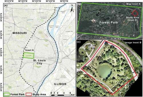
The study area is located within a large public park, Forest Park, situated amidst an urban environment within the city of St. Louis, Missouri, USA. Forest Park occupies 523 hectares (ha) of varied land cover/land use types and consists of more than 240 tree species scattered throughout (Figure 1a). Our study area occupies a 70 ha section in the northeast corner of Forest Park chosen for its diversity of tree species (Figure 1b). Designated as Round Lake, due to the large round manmade lake in the center of the section, the study area consists of 53 tree species and over 250 individual trees (Figure 1c). The climate is influenced by humid continental and humid subtropical climate zones resulting in hot and humid summers and cold winters. St. Louis experiences four distinct seasons with an average growing season of 208 days.

Figure 1. Study area location at Forest Park in St. Louis, MO, U.S.A. (a) Location of Forest Park in Saint Louis City; (b) Location of the selected study area in Forest Park; (c) UAV-based RGB imagery of the study area

2.2 Tree species data

The St. Louis City Department of Parks, Recreation and Forestry maintains a database of all trees within Forest Park, which is verified and updated annually as trees are planted and removed. The geographic location of each tree in the database is recorded using a Trimble GeoExplorer 6000 receiver with 50 cm accuracy. Additional recorded metrics include: species type, height, diameter at breast height (DBH), health condition and risk. For this study, we were interested in location and species type from the database. To validate the accuracy of the Parks, Recreation and Forestry Department inventory, we (accompanied by an arborist) conducted a test verification of tree location using a Trimble R1 GNSS Receiver with 50 cm accuracy and species type of 35 randomly selected trees throughout our study area. All of the 35 randomly selected samples matched the location and species type according to the Parks, Recreation and Forestry Department park-wide dataset. Furthermore, all individual tree point locations from the Parks, Recreation and Forestry Department database were overlayed onto a high-resolution orthomosaicked RGB dataset obtained during UAV data collection for manual verification for the presence/absence of a tree at each point location. We did not verify species type from this visual assessment. Except for a couple data points being deleted due to tree removal within the year, all individual tree point locations from the Parks, Recreation and Forestry Department database corresponded to the visual presence of trees on the RGB orthorectified imagery. Although the study area contains 53 different species, we chose to analyze tree species for which we were able to obtain a sufficient number of training samples for each species type (Table 1). Our threshold for the classification methods used here was a minimum of eight training samples, for example we excluded Silver maple from this due to only five training samples within our study area. The selected trees vary in age, size, shape within their own species sample population, thus representing similar circumstances in a typical urban setting.

Table 1. List of tree species and number of individual crown samples collected within the study area

ID	Species (common name)	Scientific Name	Samples
1	Baldcypress	Taxodium distichum	20
2	River birch	Betula nigra	19
3	Pin oak	Quercus palustris	18
4	Pecan	Carya illinoinensis	13
5	Austrian pine	Pinus nigra	9
6	Redbud	Cercis canadensis	9
7	Sycamore	Platanus occidentalis	8
	Total		96

2.3 UAV data acquisition

An aerial data campaign to collect spectral datasets from RGB, multispectral, hyperspectral, and thermal sensors was conducted on 10 September 2018. This date allowed for a leaf-on data collection to ensure the measurement of spectral properties for individual tree canopies. A separate leaf-off LiDAR data collection via UAV was conducted on 13 April 2019 to examine the 3D structural properties of individual trees. Trees were imaged with LiDAR in a leaf-off stage in order to better obtain structural parameters from individual tree branches unhindered by leaves. All sensors were flown on a DJI Matrice 600 (M600) Pro hexacopter (DJI Technology Co. Ltd., Shenzhen, China) platform (Specific information of each sensor can be found in Table 2) Prior to flights, 10 black and white painted wooden reference panels were placed throughout the study area, acting as an identifiable ground control points (GCPs) for co-registration of multiple datasets. The geographic coordinate location of the GCPs was recorded via Trimble Catalyst Differential GPS system, which provides about 10 mm and 20 mm accuracy at horizontal and vertical direction, respectively. A 4 ft x 6 ft calibrated canvas reflectance tarp with three different reflective panels (56%, 30%, and 11% reflectance) was placed within the UAV flight path to ensure it was imaged for reflectance calibration of the hyperspectral data.

Table 2. List of sensors used in this study. RGB – red, green, blue. VNIR – visible near-infrared. IR – infrared

Dataset	Sensor	Recorded info.	Spectral Properties			GSD/Point-density
RGB	Sony RX10	3 RGB bands	/			2.5 cm
Multispectral	Micasense Red-edge	5 VNIR spectral bands	Band	CW (nm)	BW (nm)	5.5 cm
			Blue	475	32
			Green	560	27
			Red	668	14
			Rededge	717	12
			NIR	842	57
Hyperspectral	Headwall Hyperspec Nano	269 VNIR spectral bands	400–1000 nm with FWHM of 6 nm			5 cm
LiDAR	Velodyne HDL-32	LAS point cloud	/			900 pts/m^2
Thermal	ICI 8640 P-series	1 thermal IR band	7–14 µm			10 cm
*GSD: ground sampling distances. RGB, multispectral, hyperspectral and thermal data were collected at 80 meters, and LiDAR data was collected at 65 meters; CW: Central Wavelength, BW: band width; FWHM: full width at half maximum, nm: nanometer, µm: micrometer.

All spectral data collection flights were planned using UgCS (SPH Engineering SIA, Latvia) flight planning software, which allows for precise programming of flight parameters based on the imaging specifications of a designated sensor. Similarly, LiDAR data collection flights were planned using Phoenix LiDAR FlightPlanner software (Phoenix LiDAR Systems, Los Angeles, California, USA), which allows for tailored flight programming for various LiDAR sensor package systems. All flight plans were designed using an overlapping “lawn mower” pattern to ensure sufficient overlying coverage of consecutive flight lines to allow for effective post-processing of mosaicked datasets. Spectral data collection missions were flown at a height of 80 m with each subsequent line overlapping the previous, also referred to as side-lap, by 80% and a forward lap of 80%, with the exception of the line scanning hyperspectral camera, which was collected at a 40% side-lap. To stay within sensor maximum effective range, the LiDAR data collection mission was flown at a height of 65 m with a side-lap of 80%. It has been demonstrated that a minimum side-lap of 80% provides sufficient image redundancy for effective orthomosaicking of aerial datasets (Maimaitijiang et al. 2019).

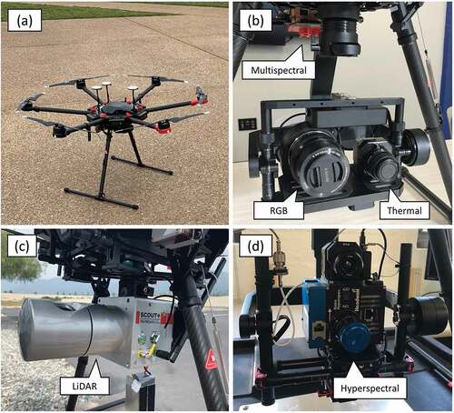
Three DJI M600 Pro UAV platforms (Figure 2a) were utilized to fly the suite of sensors outlined in Table 2. The first platform carried a Sony RX10 (Sony Corporation, Japan; RGB imagery) with ICI 8640 P-series (Infrared Cameras Inc., Beaumont, TX, USA) thermal camera mounted on a three-axis gimbal (Figure 2b). Additionally, a Micasense RedEdge-M multispectral camera (MicaSense, Inc., Seattle, USA) was hard-mounted to the platform frame. The second was equipped with a Headwall Photonics Nano-Hyperspec sensor (Headwall Photonics Inc., MA, U.S.) with 269 spectral bands in the VNIR (visible and near infrared) spectral range (400–1000 nm) and FLIR Vue Pro R 640 (FLIR Systems, Wilsonville, OR, USA) thermal camera mounted on a three-axis gimbal (Figure 2d). While both ICI and FLIR thermal cameras imaged the study area, the ICI dataset was chosen due to improved performance in previous vegetation research (Sagan et al. 2019a). The third platform was integrated with a Phoenix Scout-32 system (Phoenix LiDAR Systems, Los Angeles, California, USA) that consisted of a Velodyne HDL-32 LiDAR sensor and a Sony A7R II RGB camera (Figure 2c). The Sony A7R RGB images were strictly used for colorization of the LiDAR point cloud.

Figure 2. UAV platform and sensors utilized in this study: a) DJI M600 Pro hexacopter UAV platform; b) Micasense RedEdge-M multispectral camera, ICI 8640 P-series thermal infrared camera, and Sony RX10 RGB camera; c) Velodyne HDL-32 LiDAR sensor; d) Headwall Photonics Nano-Hyperspec sensor

2.4 UAV data preprocessing

RGB, multispectral, and thermal datasets were processed using Pix4Dmapper software (Pix4D SA, Lausanne, Switzerland), which orthorectifies and mosaicks a collection of images to create a single image of a captured study area. Pix4D is designed to process UAV data through the use of photogrammetry and computer vision techniques with user-defined parameters to produce optimal mosaics. Prior to mosaicking the thermal dataset, radiometric calibration was performed using IR-Flash software provided by the manufacturer. The IR-Flash software uses batch processing to convert at-sensor radiometric temperature to surface temperature in degrees Celsius (°C) given user-defined target and environmental condition parameters (Li et al. 2019; Maimaitijiang et al 2020a; Sagan et al. 2019a). Pix4D provides automatic radiometric calibration to reflectance for the Micasense multispectral images using sun irradiance information from a sensor module attached at the top of the UAV in conjunction with calibrated albedo values for each band obtained from a radiometric calibration target from the manufacturer.

Unlike the other spectral sensors in this study that collect a series of consecutive single images, the Headwall Nano-Hyperspec is a push broom scanner that collects data using a line of detectors aligned perpendicular to the flight direction. Sometimes referred to as linear array sensors, push broom scanners record data one line at a time with all pixels in that line recorded simultaneously. Even with the Nano-Hyperspec mounted on a three-axis gimbal for improved stability, slight fluctuations in speed and balance of the UAV platform during flight affect the consistency of the collected data cube. The hyperspectral dataset was processed using SpectralView software provided by the manufacturer. The raw data cube is converted to a radiance cube using factory calibration data along with exposure time and dark reference information recorded prior to flight. The radiance cube is then converted to reflectance using manufacturer calibrated reflectance values for the imaged reflectance tarp. Atmospheric correction was not applied here as UAV data is far less influenced by atmospheric effects due to the proximity of data collection to the ground. In order to compensate for this, calibration panels were utilized to calibrate data to surface reflectance. After reflectance conversion, the data cube is orthorectified using acceleration and rotation information recorded by the inertial measurement unit (IMU) onboard the sensory during flight. A 10 m digital elevation model (DEM) obtained from the Missouri Spatial Data Information Service and flight altitude were used to account for geometric distortion, while IMU/GPS offsets for pitch/roll/yaw are manually input to adjust for image correction and orientation. Due to the push broom collection nature of the sensor, the output of this process was 12 individual ortho-rectified flight lines.

LiDAR data processing was conducted using LiDARMill, a cloud-based LiDAR data processing application provided via subscription from the manufacturer (www.phoenixlidar.com/lidarmill, Phoenix LiDAR Systems, Los Angeles, California, USA). LiDARMill combines information from a Novatel GNSS ground reference station set up during the flight with IMU data onboard the sensor during collection to generate a smoothed best estimate of trajectory (SBET). The SBET provides a smooth and accurate flight trajectory, which allows for precise positioning of LiDAR point cloud data. The LiDAR sensor manufacturer reports a ± 2 cm accuracy for data points. The application uses automated detection methods to remove turns during data collection, leaving the more accurate straight data collection flight lines while reducing data volume and, subsequently, processing time. Finally, LiDARMill outputs a classified (ground/non-ground) LAS file, which is an industry standard file format for the interchange of LiDAR point cloud data.

2.5 Image co-registration

Image co-registration is the process of geometrically aligning two or more images to merge corresponding pixels that symbolize the same location on the ground (Kim, Lee, and Ra 2008; Feng et al. 2019). Co-registration was performed using ENVI 5.4.1 software (Exelis Visual Information Solutions, Boulder, CO, USA) which builds a geometric relationship between a base image and the aligning image based upon manually delineated matching tie points representing the same object in both images. Tie points included the placed black and white painted wooden reference panels along with distinct land features (e.g. road/path intersections, benches, man-made features, etc.) that were evenly distributed throughout the study area.

The mosaicked RGB dataset collected on 10 September 2018 from the Sony RX10 camera served as the base image for image to image co-registration. The multispectral, hyperspectral, thermal, and LiDAR raster datasets were co-registered to the RGB mosaic using a second-order polynomial warping parameter. A minimum of 25 tie points were selected for each image pairing and a root mean squared error (RMSE) of about 0.1 m for RGB data, and 0.2 m for multispectral and thermal data, and about 0.80 m for hyperspectral data. . Due to the push broom collection nature of the hyperspectral camera, the 12 orthorectified reflectance flight lines were registered individually to the RGB base image. Following co-registration, the hyperspectral reflectance flight lines were mosaicked into one single reflectance raster using the ENVI software.

3. Methods

3.1 Tree crown delineation

Individual tree crown samples are needed for training and testing of classification algorithms. Manually depicting individual tree crowns via high-resolution imagery is time consuming and costly. Detection and delineation of individual tree canopies using automated segmentation techniques facilitate analysis of individual tree biophysical traits (Ke and Quackenbush 2011; Jakubowski et al. 2013). For this study, we adopted a watershed segmentation technique which has proven an effective method for individual tree crown delineation (Ayrey et al. 2017; Panagiotidis et al. 2017). Watershed segmentation is inspired from the geographical watershed pouring scheme based on a topographic landscape with ridges as high regions and valleys as low regions. In place of topography, a canopy height model (CHM) raster derived from the LiDAR point cloud was used. The CHM was created by subtracting the digital terrain model (DTM) raster from the digital surface model (DSM) raster (Figure 3). The DSM raster represents the height of all LiDAR return points in a scene, whereas the DTM raster represents all ground points within a scene. The DSM was created by rasterizing the point clouds using ArcGIS pro software program (ESRI, Redlands, California, USA); point clouds were classified as ground and non-ground portion, and the DTM was created by rasterizing the non-ground point clouds. The pixel values of non-canopy open areas and ground in CHM are zero or close to zero, and those pixels were segmented out by thresholding method, and the final CHM represents tree height. Similar to topographic values, higher tree height pixel values are interpreted as “high” regions, such as ridges, and lower tree height pixel values are interpreted as “low” regions, such as valleys. Understanding the gradient between high/low values and determining where two slopes meet at a low point, can help distinguish the edges of tree canopies, particularly interlocking canopies.

Figure 3. Workflow diagram of UAV data pre-processing, feature extraction & combinations, classification model building and evaluation (MSI represents multispectral imagery/data; HSI represents hyperspectral imagery/data)

The watershed segmentation algorithm was created and implemented as a custom Python script. First, treetops were identified using a local maxima filter at which markers were placed to simulate high topographical features. A Gaussian filter based on a two-dimensional Gaussian distribution was applied to remove detail from the image so that the application of a local minima operation would avoid false positives. Next, a dilated convolution morphological operation was applied to prevent over segmentation. Morphological dilation makes objects more visible and fills in small holes in objects. Finally, the algorithm simulated flooding of the basins from the markers until flooding met on watershed lines of adjacent features, which represent the edges of tree crowns. Segmented polygons corresponding to the location of the selected seven tree species chosen for this study (Table 1) were retained for classification analysis.

This study adopts a classification strategy that classifies individual tree objects (delineated image cubes) rather than a scene classification. Unlike traditional remote sensing image classification or mapping, where all objects within an image scene are classified as part of the whole image, the method here performs individual image-based classification, where each image contains only one object (tree). Each segmented tree crown represents one object/image. This method was chosen due to the objective of classifying specific selected species rather than all objects within the scene (study area) together.

3.2 Feature extraction

In an effort to examine the contributions of various sensors for tree species classification using a simple feature-level data fusion approach (Hartling et al. 2019; Maimaitijiang et al. 2020b) raster feature layers extracted from different dataset were layer-stacked to establish a multilayered data cube, and used as input imagery for classifiers. Five sets of features were considered in this study: 1) VNIR multispectral bands; 2) VNIR hyperspectral minimum noise fraction (MNF) bands; 3) LiDAR extracted features; 4) crown temperature extracted from thermal imagery; and 5) vegetation indices from the respective spectral sensors. Spectral information from the multispectral and hyperspectral cameras was combined with structural information from the LiDAR, temperature from thermal sensor, and vegetation indices derived from the reflectance data as outlined in Table 3. The objective was to investigate the contribution of spectral, structural, and temperature information for tree species classification. All datasets were resampled to a spatial resolution of 10 cm in order to compare all datasets at a common resolution.

Table 3. List of features used for classification

Features	Feature Type	Number of feature bands
Multispectral VNIR	Spectral	5
Hyperspectral VNIR	Spectral	49
Vegetation indices (VIs)	Spectral	10
Thermal	Thermal	1
LiDAR	Structural	18

3.2.1 Vegetation indices

Studies have demonstrated that the incorporation of vegetation indices with individual spectral band information has improved overall tree species classification (Maschler, Atzberger, and Immitzer 2018; Cross et al. 2019) and, in some cases, have proven more important than structural features (Franklin, Ahmed, and Williams 2017). Vegetation has a unique spectral signature with a strong reflectance in the near-infrared (NIR) spectral region in comparison to its distinct absorption in the red spectrum as a result of chlorophyll pigment necessary for photosynthesis. For this study, 10 commonly used vegetation indices extracted from both multispectral and hyperspectral imagery were used as input variables for classification models and investigated for their potential to discriminate the spectral variation between the selected tree species (Table 4). These vegetation indices were created using band calculations within the ENVI 5.4.1 software (Sagan et al. 2019b)

Table 4. Vegetation indices selected for classification*

Vegetation Index Name	Abbreviation	Formula	References
Atmospherically Resistant Vegetation Index	ARVI	$\frac{NIR-RED-y\left(RED-BLUE\right)}{NIR+RED-y\left(RED-BLUE\right)}$	(Kaufman and Tanre 1992)
Canopy Chlorophyll Content Index	CCCI	$\frac{\frac{NIR-RedEdge}{NIR+RedEdge}}{\frac{NIR-RED}{NIR+RED}}$	(Fitzgerald, Rodriguez, and O’Leary 2010, Felderhof and Gillieson 2014)
Enhanced Vegetation Index	EVI	2.5 $\frac{NIR-RED}{NIR+6RED-7.5BLUE+1}$	(Glenn et al. 2008)
Green Normalized Difference Vegetation Index	GNDVI	$\frac{NIR-GREEN}{NIR+GREEN}$	(Gitelson, Merzlyak, and Lichtenthaler 1996, Lymburner, Beggs, and Jacobson 2000, Ismail, Mutanga, and Bob 2007)
Normalized Difference Red Edge Index	NDRE	$\frac{NIR-RedEdge}{NIR+RedEdge}$	(Eitel et al. 2011, Waser, Küchler et al. 2014)
Normalized Difference Vegetation Index	NDVI	$\frac{NIR-RED}{NIR+RED}$	(Gamon et al. 1995, Gould 2000, Zimmermann et al. 2007)
Plant Senescence Reflectance Index	PSRI	$\frac{RED-BLUE}{RedEdge}$	(Sims and Gamon 2002)
Pigment Specific Simple Ratio (Chlorophyll a)	PSSRa	$\frac{NIR}{RED}$	(Blackburn 1998, Sims and Gamon 2002)
Soil Adjusted Vegetation Index	SAVI	$\frac{NIR1-RED}{NIR1+RED+L}$ $\times \left(1+L\right)$	(Huete 1988, Lymburner et al. 2000)
Visible Atmospherically Resistant Indices – Red Edge	VARI-Red Edge	$\frac{RedEdge-RED}{RedEdge+RED}$	(Gitelson et al. 2002)

*NIR, RED, BLUE, GREEN, Red Edge are the near-infrared, red, blue green and red-edge spectral regions/bands of the hyperspectral/multispectral imagery, respectively. L is a soil brightness correction factor of the SAVI index, a commonly employed value 0.5 was used for the calculation of SAVI in this work.

3.2.2 LiDAR point-cloud feature extraction

Advances in high-precision UAV-mounted LiDAR instruments led to their utilization for high-density and survey grade 3D point clouds in forestry applications (Sankey et al. 2017; Liu et al. 2018; Cao et al. 2019). LiDAR can be used to extract a wide range of tree structural attributes such as tree height, stem diameter, and crown density (Wasser et al. 2013, Kwak et al. 2007). A total of 18 structural features were extracted from the LiDAR point cloud and created as raster bands for data fusion (Table 5). The CHM generated for crown segmentation was the first band of structural feature representing the maximum height of each pixel within the tree crown. Second, a LiDAR intensity return raster band was created, which is a representation of the reflectivity and surface composition of the object on the ground and can be useful in distinguishing differences between tree species. The next five bands were calculated using statistical summaries of the corresponding CHM raster cells found within each individual tree crown polygon: mean, kurtosis, skewness, standard deviation and median absolute deviation (Table 5). The remaining eleven structural statistics represent the height at which the specified percentile of points in the cell occur above the ground. These percentiles were calculated at 99%, 95%, 90%, 80%, 70%, 60%, 50%, 40%, 30%, 20%, and 10%. Point cloud-derived features were used as input variables for classification models. Point cloud statistics and height metrics were generated using the LAS height metrics tool within ArcGIS Desktop 10.5.1 (ESRI, Redlands, CA, USA). Examining the statistics of each pixel throughout each sample polygon in the context of neighboring pixels can infer overall shape and structural characteristics of individual tree canopies which are unique to each species.

Table 5. Structural features extracted from LiDAR point cloud

Feature name	Description	Extracted from	Total bands
Elevation	Value represents maximum height value in meters above ground	LAS point cloud	1
Intensity	Average return strength of laser pulses within cell	LAS point cloud	1
Mean	Average height of LAS points within cell	LAS point cloud	1
Kurtosis	Magnitude of change in height of LAS points	LAS point cloud	1
Skewness	Direction of bias in deviations from the nominal height of LAS points	LAS point cloud	1
Standard deviation	Variation of height of LAS points within cell	LAS point cloud	1
Mean standard deviation	Median value of deviation from the median height of LAS points	LAS point cloud	1
Height percentile	Height where percentage of points in the cell occur above the ground: 99%, 95%, 90%, 80%, 70%, 60%, 50%, 40%, 30%, 20%, 10%	LAS point cloud	11
		Total	18

3.2.3 Hyperspectral dimensionality reduction – MNF transform

Compared to the five bands of the Micasense Red-Edge multispectral camera (Blue – 475 nm, Green – 560 nm, Red – 668 nm, Red-edge – 717 nm, NIR – 842 nm), the Headwall Nano-hyperspec camera records 269 raw VNIR spectral bands at 4 nm increments. In order to reduce dimensionality by minimizing noise and, consequently, scaling down the number of bands, MNF (Minimum Noise Fraction) transform was performed on the raw hyperspectral reflectance bands. MNF is a popular technique for denoising hyperspectral imagery (Clark and Kilham 2016; Onojeghuo and Onojeghuo 2017) and has demonstrated success over other dimensionality reduction techniques such as principal component analysis (PCA) (Luo et al. 2016; Priyadarshini et al. 2019). The MNF uses a linear transformation technique that performs two cascaded PCAs in order to maximize the signal-to-noise ratio. The first PCA decorrelates and rescales noise in the data, followed by a second PCA on the transformed noised-whitened data with no band to band correlations. The output of the MNF is a series of modified bands ordered by eigenvalues, where higher eigenvalues contain more information and lower values indicate more noise. The original 269 reflectance bands were reduced to 49 MNF bands, which account for 70% of the relevant information contained in the hyperspectral imagery for tree species classification. Both MNF and PCA results were tested and MNF performed better than using PCA alone for dimensionality reduction in terms of tree classification accuracy.

3.3 Classification and validation

RF and SVM were chosen as the classifiers for this study due to their ability to handle high-dimensional datasets and demonstrated success for tree species classification (Immitzer, Atzberger, and Koukal 2012a; Li et al. 2015; Liu et al. 2017). . It is worth notating that, to examine and compare the potential of multispectral and hyperspectral datasets, the classification performance of each dataset, as well as combination of each dataset with features derived from other sensors (i.e. LiDAR and thermal) was evaluated, respectively. The dataset combination approaches for tree species classification is outlined in Table 6.

Table 6. Combination methods of different features/datasets and corresponding feature numbers of each method

Spectral sensor used	VNIR	VNIR+VIs	VNIR+LiDAR	VNIR+LiDAR+Thermal	VNIR+LiDAR+Thermal+VIs
Multispectral dataset	5	15	23	24	34
Hyperspectral dataset	49	59	67	68	78

Note: VNIR multispectral – 5 VNIR reflectance bands, VNIR hyperspectral – 49 bands after applying MNF-based dimension reduction, VIs – 10 vegetation indices selected for this experiment and calculated for both multispectral and hyperspectral dataset, LiDAR – 18 structural features derived from LiDAR point cloud, Thermal – single band representing canopy temperature in Celsius degree.

3.3.1 Random Forest

The RF classification approach utilizes a non-parametric ensemble method that generates several decision trees over various random sub-samples of the dataset and assigns a class to a sample based upon a majority vote from the collective decision tree outputs for that sample (Breiman 2001). Decision trees are built from a random sample of the data and utilizes bootstrap aggregation to randomly select input variables at each split in the decision tree growth. This randomness in selection of training sample and feature selection allows for decision trees that are relatively uncorrelated and the use of average voting increases predictive accuracy while decreases over-fitting. The RF classifier was implemented using the scikit-learn machine learning library in Python. A grid-search and k-fold cross-validation approach were employed to determine the optimal parameters during the model training phase (Maimaitijiang et al. 2020b). For RF classifier, the number of trees parameter which decides how many trees the RF considers at each split was set between 1 and 500 with a 50 increment, and the max_features parameter was automatically selected from “auto,” “sqrt’,” “log2” methods.

3.3.2 Support Vector Machine

SVM is a non-probabilistic binary linear machine learning classifier that builds an optimal hyperplane through n-dimensional space that separates classes by maximizing the margin between any data point within the training set and the hyperplane (Cortes and Vapnik 1995). Due to its ability to find the optimal hyperplane in high-dimensional feature space, SVM is a popular machine learning classifier for complex datasets. SVM uses a supervised learning model based upon a user-defined kernel function and optimized parameters to minimize the upper limit of the classification error of the training data and the optimal hyperplane. The SVM classifier was implemented using the scikit-learn machine learning library in Python. The SVM algorithm utilized Radial Basis Function Kernel (RBF) as the kernel function with a five-fold grid search cross-validation approach to determine optimal classifier parameters: C and gamma. The C parameter acts as the degree of tolerance when searching for the decision function, the optimized C value was selected from 0.1, 1, 10, 100, 1000 values. The gamma parameter determines the influence of a single training parameter on the decision function, it was selected from 1, 0.1, 0.01, 0.001, 0.0001 values. The optimal tuned parameters for C and gamma parameters were then applied to create a best model.

3.3.3 Classifier evaluation

Classifier performance was validated using a using leave-one-out cross-validation (LOOCV) method. LOOCV is a k-fold cross-validation approach where the number of folds equals the number of samples. Each sample is used once for testing, with all other samples are used for training. Therefore, each classifier model is trained on all data samples except for the left-out data sample for testing, which is then used for validation. Considering the 96 data samples representing individual tree crowns (Table 1), each model was trained 96 times. LOOCV is robust technique that incorporates all available information while not relying on a specific number of data samples, and has demonstrated success with small samples (Brovelli et al. 2008; Sothe et al. 2019). Given the limited number of samples of each tree species imaged within the confined UAV flight coverage area, LOOCV was chosen as the most effective method for assessing model accuracy.

Overall accuracy (OA) provides a percentage measure of the proportion of correctly predicted tree species to the total number of samples. User’s accuracy (UA) is the probability that a sample predicted to be in a certain class is actually that class. UA is calculated by dividing the number of correctly classified samples by the total number of samples classified as that particular class. Producer’s accuracy (PA) is the probability that a sample in an image is in that particular class. PA is based on the fraction of correctly predicted samples to the total number of samples for that species. The kappa index is a measure of the extent to which the predicted accuracy of the classifier compares to ground truth accuracy, controlling for accuracy achieved by random chance. Kappa index values range from zero to one and can be interpreted according to strength of agreement between predicted and ground truth values in relation to the following scale: 0.01–0.20 slight; 0.21–0.40 fair; 0.41–0.60 moderate; 0.61–0.80 substantial; 0.81–1.00 almost perfect (Landis and Koch 1977). The procedures from data pre-processing, feature extraction, feature selection, model training and evaluation are displayed in Figure 3.

4 Results

4.1 Tree crown delineation

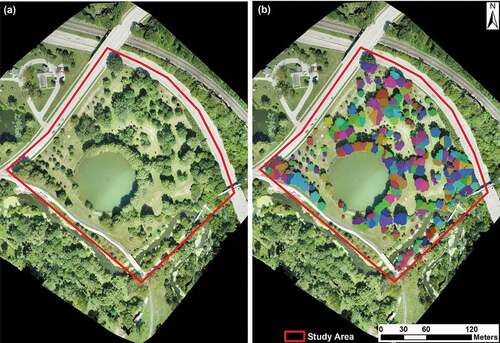
Figure 4 (b) exhibits the individual tree crown delineation results using the watershed segmentation algorithm based on LiDAR point cloud-derived CHM. Each color patch in Figure 4(b) represents one tree crown/object. Compared to the tree distribution in the study area shown in UAV RGB imagery (Figure 4(a)), the majority of trees were successfully identified and tree crowns were correctly delineated. However, boundaries of some tree crowns were not correctly detected, particularly at the area with very high tree density; thus, boundaries of those trees were manually adjusted and corrected to derive accurate tree crowns. The extracted tree crown boundaries were then overlaid with multisensory datasets and features to generate individual tree data cubes for classification.

Figure 4. Tree crown delineation results based on Canopy Height Model using watershed segmentation algorithm. (a) UAV-based RGB imagery of the study area; (b) Segmented tree crowns represented by different color patches

4.2 Species differentiation by sensor type

4.2.1 Multispectral and hyperspectral

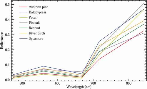
The numerous bands recorded by the hyperspectral provide more spectral separability between species, most noticeably in the NIR region (Figure 5). All species exhibited a general vegetation reflectance curve with a slight peak in the green (~550 nm) region, low valleys in the blue (~450 nm) and red (~670 nm) regions and a large spike in the NIR (~ >720 nm) region. Pin oak demonstrated the highest values in the NIR region on both hyperspectral (Figure 5) and multispectral (Figure 6) sensors. Of all the mean reflectance curves, sycamore stands out as it does not resemble a typical healthy vegetation curve. Both hyperspectral (Figure 5) and multispectral (Figure 6) reflectance curves for sycamore, demonstrate a flattened transition from the green to red region, as well as a shallower transition into the NIR region, which is particularly evident in the hyperspectral reflectance curve (Figure 5).

Figure 5. Hyperspectral reflectance profiles for each species type. Spectral profiles represent the mean reflectance curve of all samples within a species population. Hyperspectral reflectance profiles provide more spectral separability between species due to increased spectral resolution. Distinguishability between species is most apparent in the NIR region

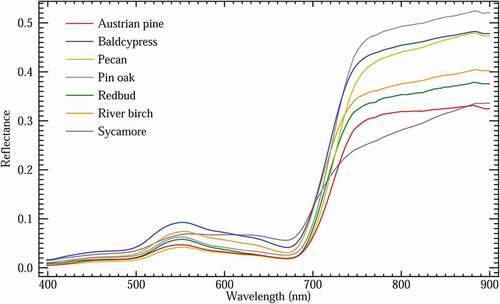
Figure 6. Multispectral reflectance profiles for each species type. Spectral profiles represent the mean reflectance curve of all samples within a species population. Sycamore stands out most among the spectral signatures of the species studied as demonstrated both hyperspectral and multispectral data. A flattened transition from the green to red region, as well as a shallower transition into the NIR region is consistent with the senescence stage observed with sycamore species when the data was collected

4.2.2 Thermal

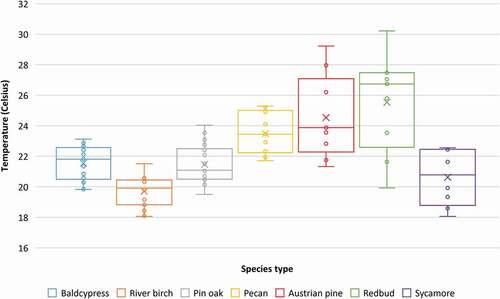
Figure 7 demonstrates the mean temperature values across each individual tree crown within a species population. Redbud species demonstrated a relatively higher overall mean temperature compared to the other species, as indicated by the “X” in the box plots (Figure 7). Contrastingly, river birch exhibited a relatively lower overall mean temperature compared to the other species (Figure 7).

Figure 7. Box and whisker plots depicting mean temperature values in degrees Celsius extracted from thermal infrared imagery for each individual tree sample by species type. Circles represent mean temperature for all cells within a single crown. The “X” represents the mean temperature value for all samples from the respective species dataset

4.2.3 LiDAR

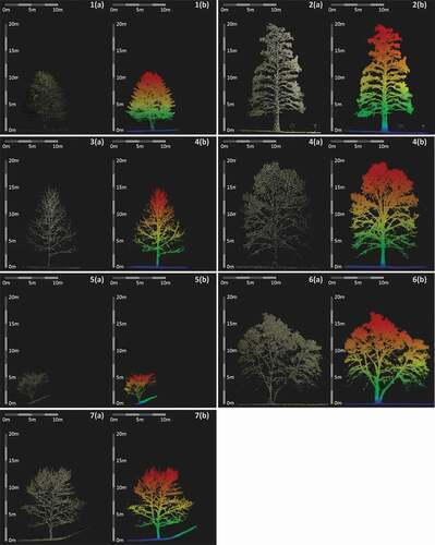
Figure 8 depicts the cross-sections of a LiDAR point cloud for one sample from each tree species collected for this study. A mature sample from each species type was chosen from our study site to get close to a standard of the respective species and highlight the differences in height, shape and structure between the studied species. Visual inspection of Figure 8 illustrates distinct shape differences: Austrian pine, baldcypress and pecan have conical shapes; pin oak has a more oblong oval shape; river birch and sycamore have more rounded crowns; and redbud has a heart or v-shaped crown. Size differences are also evident in the cross-sections of each species within Figure 8. Baldcypress (2) and pin oak (4) are two of the tallest trees from the studied species, while redbud (5) is the smallest. River birch (6) represents one of the widest/broadest tree crowns at maturity of the studies species.

Figure 8. LiDAR point cloud cross-sections of sampled tree species. A – colorized point cloud. B – point cloud colorized by height. (1) Austrian pine; (2) baldcypress; (3) pecan; (4) pin oak; (5) redbud; (6) river birch; (7) sycamore

In this study, mean height (Figure 9) and mean intensity values (Figure 10) within individual tree canopies were examined between species. LiDAR intensity is another metric typically incorporated in tree species classification research. Intensity represents the amount of energy reflected from a target as a relative measure of the return signal strength of each laser pulse. Values for intensity depend on a variety of factors, such as target reflectivity, directional reflectance properties, sensor height, atmospheric conditions and laser settings (Baltsavias 1999). LiDAR intensity data is influenced by crown density and gaps in the crown, which can help provide distinction between species (Holmgren and Persson 2004).

Figure 9. Box and whisker plots depicting mean height values in meters extracted from LiDAR point cloud for each individual tree sample by species type. Circles represent mean height for all cells within a single crown. The “X” represents the mean height value for all samples from the respective species dataset

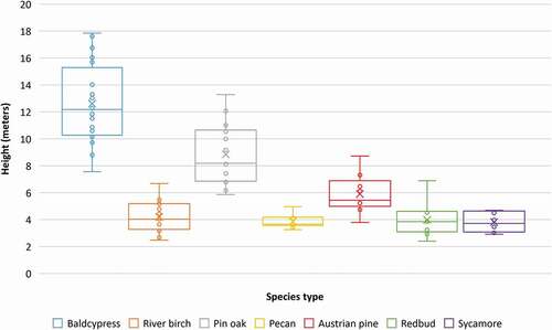
Figure 10. Box and whisker plots depicting mean intensity values extracted from LiDAR point cloud for each individual tree sample by species type. Circles represent mean intensity for all cells within a single crown. The “X” represents the mean intensity value for all samples within respective species dataset

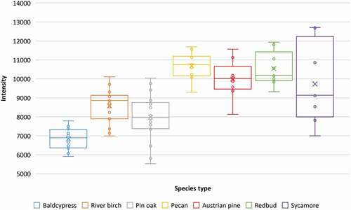
According to Figure 9, it is apparent that baldcypress, river birch and Austrian pine samples were generally taller than the other species, which corresponds to the standard height characteristics for species within this study, with the exception of sycamore. With the exception of the lone conifer species of Austrian pine, all other tree species were deciduous and without green leaves/foliage when imaged with LiDAR in a leaf-off stage. Therefore, intensity values in Figure 9 are more likely related to the branch structure and reflective properties of the branches of each species, with exception of the Austrian pine which retains its needles all year. Baldcypress, river birch and pin oak demonstrate relatively lower mean intensity for the species population, with baldcypress, as a species, exhibiting the lowest intensity values, generally (Figure 10).

4.3 Overall classification accuracy

The incorporation of additional features to the initial VNIR reflectance bands for both multispectral and hyperspectral datasets increased overall classification accuracy across both classifiers. The RF classifier outperformed the SVM classifier across all feature dataset combinations, as well as when using only multispectral-visible near-infrared (MSI-VNIR) or hyperspectral-visible near-infrared (HSI-VNIR) dataset. Under RF MSI-VNIR dataset, overall accuracy (OA) increased from 55.2% for the VNIR reflectance bands only to 81.3% using all features. However, spectral information derived from the hyperspectral sensor produced an initial 70.8% OA using only reflectance information from the 49 MNF hyperspectral bands with RF. The highest OA of all classification tests was achieved with the RF classifier and the full feature dataset combination (VNIR+LiDAR+Thermal+VIs) using hyperspectral information with an OA of 83.3% (Table 7).

Table 7. Classification results when using different feature set combinations and RF classifier

Spectral Sensor	Metric	VNIR	VNIR+VIs	VNIR+LiDAR	VNIR+LiDAR+Thermal	VNIR+LiDAR+Thermal+VIs
Multispectral	OA (%)	55.2	68.8	75.0	75.0	81.3
	Kappa	0.45	0.62	0.69	0.70	0.77
Hyperspectral	OA (%)	70.8	74.0	76.0	81.3	83.3
	Kappa	0.64	0.68	0.71	0.77	0.80

The SVM classifier demonstrated a similar, albeit lower, trend, with OA starting at 53.1% and 60.4% using only MSI-VNIR or HSI-VNIR reflectance bands, respectively. Under the SVM classifier, the incorporation of all feature information (VNIR+LiDAR+Thermal+VIs) to MSI-VNIR spectral bands obtained the highest OAs of 72.9%, and 76.0% when adding all features to HSI-VNIR spectral bands (Table 8).

Table 8. Classification results when using different feature set combinations and SVM classifier

Spectral Sensor	Metric	VNIR	VNIR+VIs	VNIR+LiDAR	VNIR+LiDAR+Thermal	VNIR+LiDAR+Thermal+VIs
Multispectral	OA (%)	53.1	61.5	64.6	66.7	72.9
	Kappa	0.42	0.52	0.57	0.60	0.67
Hyperspectral	OA (%)	60.4	64.6	67.7	74.0	76.0
	Kappa	0.51	0.57	0.60	0.69	0.71

The incorporation of different feature types (spectral, structural, or thermal) produced varied OA results depending on the sensor from which the spectral information was derived – multispectral or hyperspectral. The tests with multispectral-derived spectral features experienced the largest difference in OA from VNIR reflectance bands only to the combination of all features with an increase of 26.1% and 19.8% for RF and SVM classifiers, respectively. Structural features from LiDAR produced a larger increase in OA over VIs when added to information from VNIR reflectance bands only for both MSI-VNIR and HSI-VNIR datasets and across both RF and SVM classifiers. Furthermore, the incorporation of either LiDAR or VI features generated much higher increases in OA for the MSI-VNIR reflectance bands over the HSI-VNIR. The feature combination dataset of MSI-VNIR reflectance bands with LiDAR features resulted in the larger OA increases over VIs with OA gains of 19.8% and 11.5% for RF and SVM, respectively. Despite being only one band of information, the sole thermal feature increased OA when added to VNIR and LiDAR features for both MSI-VNIR & HSI-VNIR and both classifiers.

Kappa indices increased with the incorporation of each additional feature dataset across both MSI-VNIR and HSI-VNIR cases as well as both RF and SVM classifiers. The highest kappa index of 0.80 was achieved using the RF classifier with all features in the case of using hyperspectral imagery as the spectral dataset (Table 7). Kappa indices were higher for all hyperspectral feature dataset combinations over the equivalent multispectral feature combinations for both RF and SVM.

4.4 Classification accuracy for each tree species

Figure 11 and Figure 12 demonstrate the producer accuracies (PA) by species for each feature dataset combination using the RF classifier. Results from the RF classifier were chosen due to its improved overall classification accuracies in every category over SVM. Overall, larger sample size resulted in higher PAs. Specifically, tree species with more than ten samples (baldcypress, river birch, pin oak and pecan (Table 1)) exhibited significantly higher PAs, whereas species with less than 10 samples (Austrian pine, redbud and sycamore (Table 1)) demonstrated considerably lower PAs. With the exception of river birch using only the five multispectral reflectance bands (Figure 12), all species with more than 10 samples achieved PAs of over 80% using the RF classifier.

Figure 11. Producer accuracies (PA) for RF classifier using hyperspectral-derived spectral features. Species abbreviations: BC- baldcypress; RB- river birch; PO- pin oak; PE- pecan; AP – Austrian pine; RD – redbud; SY- sycamore

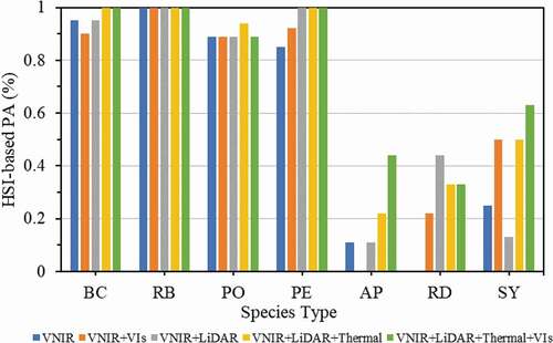
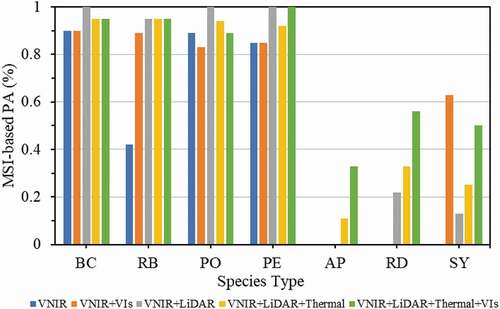
Figure 12. Producer accuracies (PA) for RF classifier using multispectral-derived spectral features. Species abbreviations: BC- baldcypress; RB- river birch; PO- pin oak; PE- pecan; AP – Austrian pine; RD – redbud; SY- sycamore

In the case of using HSI-VNIR-based spectral features (Figure 11) and species with more than 10 samples, the addition of LiDAR and thermal features to the spectral features maintained or improved PA, in general. For tree species with less than 10 samples and HSI-VNIR derived spectral features (Figure 11), Austrian pine and sycamore achieved highest PAs for their individual species of 44.4% and 62.5%, respectively, when including all feature datasets; whereas, redbud demonstrated its highest PA of 44.4% when only combining hyperspectral MNF reflectance bands and LiDAR features.

Comparing results for the MSI-VNIR derived spectral features and RF in Figure 12, baldcypress and pin oak provided the highest PAs for feature combination of VNIR reflectance bands with LiDAR features and match the PA when incorporating all features for river birch and pecan, of the tree species with over ten samples. For species with less than ten samples (Table 1), PAs were zero when only using the five multispectral VNIR reflectance bands and did not improve for Austrian pine or redbud when adding the VIs to the VNIR bands. However, Austrian pine and redbud achieved their highest individual UAs of 33% and 56%, respectively, when including all features into the RF classifier. Notably, sycamore exhibited the highest UA of 63% when testing the feature combination of VNIR reflectance bands and VIs with RF.

Figure 13 and Figure 14 demonstrate the user accuracies (UA) by species for each feature dataset combination using the RF classifier. In the case of using HSI-VNIR as spectral dataset, tree species with larger sample size (i.e. baldcypress, river birch, pin oak and pecan) yielded relatively higher UAs in most of the feature combination cases (Figure 13), especially the UA of pecan reached 100% under all feature combination sceneries. Tree species Austrian pine and sycamore which have smaller sample size produced lower UAs; Although, with lower sample size, sycamore trees generated 100% UAs in most of the cases. Figure 14 displays the UAs in the case of using MSI-VNIR as spectral dataset, overall, UAs are lower than those in the case of using HSI-VNIR dataset; additionally, similar trend that larger sample size produced higher accuracies was observed as well.

Figure 13. User accuracies for RF classifier using hyperspectral-derived spectral features. Species abbreviations: BC- baldcypress; RB- river birch; PO- pin oak; PE- pecan; AP – Austrian pine; RD – redbud; SY- sycamore

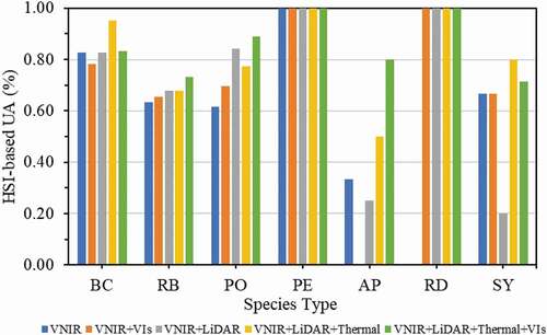
Figure 14. User accuracies for RF classifier using multispectral-derived spectral features. Species abbreviations: BC- baldcypress; RB- river birch; PO- pin oak; PE- pecan; AP – Austrian pine; RD – redbud; SY- sycamore

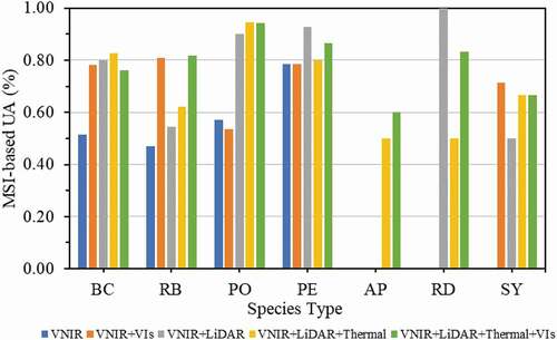
It is worth noting that, combining the LiDAR and thermal data based features to spectral features increased the UAs for most of the tree species; particularly, inclusion of LiDAR and thermal features boosted the UAs of Austrian pin and redbud from 0 to above 50%.

5 Discussion

5.1 Contribution of multisensory data fusion

The results show that the combination of hyperspectral-derived spectral features (MNF VNIR reflectance and Vis), LiDAR-based structural information and thermal datasets achieved the highest overall classification accuracy of 83.3% (Table 7). This was followed closely by the multi-spectral derived features combined with LiDAR and thermal datasets at 81.3%. Regardless of multispectral or hyperspectral-derived spectral information, the addition of LiDAR and thermal information increased overall classification accuracy across both RF and SVM classifiers. Additionally, multisensory data combination also generally improved the classification accuracies of each tree species as well.

Despite hyperspectral-derived information producing the highest overall classification accuracies, multispectral-derived information received the highest increase in classification accuracy when combined with additional information from LiDAR and thermal sensors. Examining the RF classifier, overall classification accuracy using reflectance information alone was 55.2% and 70.8% for multispectral and hyperspectral sensors, respectively. Adding information from the LiDAR and thermal sensors together increased OA to 75% and 81.3% to the multispectral and hyperspectral reflectance information, respectively, demonstrating a gain of 19.8% in accuracy from the multispectral reflectance information alone and 10.5% from the hyperspectral reflectance information alone. Incorporating VIs to the reflectance, LiDAR and thermal datasets, increased OA to 81.3% for multispectral-derived spectral information – a 26.1% increase from reflectance information alone – and increased OA to 83.3% for hyperspectral-derived spectral information – a 12.5% increase from reflectance information alone. While hyperspectral information provides more spectral separability between tree species over multispectral information, the results here demonstrate the ability of additional information from LiDAR and thermal sensors to fill that information gap needed to distinguish between species.

This study demonstrates the advantage of a multi-sensor data combination approach for tree species classification in an urban environment. The ability to extract unique features from spectral, LiDAR and thermal sensors allowed the classifiers to identify distinguishable features between species and produce higher overall accuracies when provided all feature information. To our knowledge, we do not know of research incorporating such a full spectrum of UAV-based sensors – multispectral, hyperspectral, LiDAR, thermal – to investigate tree species classification in an urban environment.

5.2 Species differentiation by sensor type

Spectral, structural and thermal information extracted from each of the sensors filled a critical information gap for certain tree species, which helped aid in improved classification accuracy. Tree species classification research has demonstrated the effectiveness of multispectral (Franklin, Ahmed, and Williams 2017; Franklin and Ahmed 2018), hyperspectral (Clark, Roberts, and Clark 2005; Ballanti et al. 2016), LiDAR (Alonzo, Bookhagen, and Roberts 2014; Sankey et al. 2017) and thermal (Lapidot et al. 2019) sensors to distinguish between species. Examining the information extracted for each species by sensor type provided context for the results of classification accuracy by species type (Figure 11 to Figure 14).

The numerous bands recorded by the hyperspectral provide more spectral separability between species, most noticeably in the NIR region (Figure 5). This potentially explains why the classifications using only spectral features, either reflectance band only information or reflectance bands with VIS, generally performed better using hyperspectral-derived spectral features (Figure 11 and Figure 13) over the multispectral-derived features (Figure 12 and Figure 14). This is apparent for river birch where the producer’s accuracy for the species was 100% for hyperspectral MNF bands compared to 42.1% for multispectral reflectance bands.

The unique flattened reflectance curve displayed by the sycamore species can be explained by the seasonal stage of the sycamore species samples within our study area. Given the date of our spectral data collection flights in early/mid-September, which falls somewhere between the end of summer and beginning of autumn seasons, the sycamore leaves were in the senescence stage and had already changed to a yellowish/brown color that was identifiable in RGB imagery. This phenomenon is potentially evident in the classification accuracies for sycamore species from Figure 5 to Figure 8, where the addition of VIs to reflectance bands produced a marked increase in accuracies. VIs are transformations or ratios of reflectance bands designed to highlight specific vegetation properties. The VIs selected for this study (Table 4) focus on the relationship between the NIR or the red-edge transitional zone into the NIR and the visible reflectance bands. The distinct reflectance curve, particularly in the NIR region, potentially provides the ability for the RF classifier to distinguish sycamore from other studied species when including VIs into the training features.

While less studied among the sensors typically employed for tree species classification, thermal infrared has previously been utilized to examine distinguishable characteristics between conifer and broadleaved tree species (Lapidot et al. 2019). River birch exhibited a relatively lower overall mean temperature for the species as compared to the others (Figure 11). This is potentially explained by the majority of species sample population located near the bank of a stream running through the southeast corner of the study area. Previous UAV research has established a connection between water resources and vegetation canopy temperature (Sagan, 2019a), suggesting the proximity of the samples to a water source could potentially lower crown temperatures. As mentioned, there was a definite distinction between species with over 10 samples (baldcypress, river birch, pin oak, and pecan) and species with less than 10 samples (Austrian pine, redbud and sycamore) when comparing classification accuracies for each species (Figure 5 to Figure 8). With the exception of redbud in the case of using hyperspectral imagery as spectral dataset (Figure 5 and Figure 7), adding the temperature feature to the hyperspectral+LiDAR features improved the RF classifier’s ability to distinguish the species with less than 10 samples. This suggests that thermal infrared features, albeit slightly, can aid in tree species classification by providing discernable information to improve classification hierarchy.

LiDAR imaging remains one of the most accurate methods for extracting 3D structural information of trees. Variables derived from LiDAR are typically statistically designed to characterize the structure of tree crowns, stems, and leaves through height distributions and intensity features. Similar research has incorporated laser pulse range and intensity return values to develop structure features such as height percentiles and standard deviation of heights for discriminating tree species (Kim et al. 2009; Ke, Quackenbush, and Im 2010; Kim, Hinckley, and Briggs 2011).

Tree crown shape can affect metrics that describe the shape of a point cloud distribution, such as skewness and kurtosis, which measure the degree of symmetry and the peakedness in distribution, respectively. LiDAR intensity is another metric typically incorporated in tree species classification research. Intensity represents the amount of energy reflected from a target as a relative measure of the return signal strength of each laser pulse. Values for intensity depend on a variety of factors, such as target reflectivity, directional reflectance properties, sensor height, atmospheric conditions and laser settings (Baltsavias 1999). LiDAR intensity data is influenced by crown density and gaps in the crown, which can help provide distinction between species (Holmgren and Persson 2004). Furthermore, broadleaf trees have been found to produce twice the intensity value over conifer trees (Song et al. 2002). Incorporation of the various height and intensity metrics derived from LiDAR can significantly improve classification hierarchy by increasing the interspecies variation represented by unique structural characteristics of different tree species.

In this study, mean height (Figure 9) and mean intensity values (Figure 10) within individual tree canopies were examined between species. According to Figure 9, it is apparent that baldcypress, river birch and Austrian pine samples were generally taller than the other species, which corresponds to the standard height characteristics for species within this study, with the exception of sycamore. Sycamore trees can grow up to 18–37 m at maturity (USDA 2020); however, the samples in our study were transplanted in 2015, which explains the lower comparative height and relatively uniform mean height values. With the exception of the lone conifer species of Austrian pine, all other tree species were deciduous and without green leaves/foliage when imaged with LiDAR in a leaf-off stage in order to better obtain structural parameters unhindered by leaves. Therefore, intensity values in Figure 10 are more likely related to the branch structure and reflective properties of the branches of each species, with exception of the Austrian pine which retains its needles all year. Baldcypress, river birch and pin oak demonstrate relatively lower mean intensity for the species population, with baldcypress, as a species, exhibiting the lowest intensity values, generally (Figure 10). The lower intensity is possibly related to the unique branch properties of the baldcypress whose crown is comprised of many slender terminal twigs that host many needlelike leaves in the spring, but in the leaf-off season are reddish-brown and somewhat rough/fibrous (USDA 2020). While this study does not investigate the influence of each LiDAR feature on classification of species by type, it highlights the ability to provide distinguishable characteristics for individual species that will help the classifiers in identifying a distinction between input classes.

5.3 Limitations and future work

One of the main challenges of individual tree species classifications is the creation of a robust training model that can be applied to multiple locations. Many factors – such as climate, soil type, resources, anthropogenic effects – can significantly affect the growing conditions of an individual tree, and also vary greatly by location. These can all influence height, shape, crown temperature, and spectral reflectance. Therefore, classifier success depends highly upon having representative training samples for species within the applied study area. Furthermore, feature selection is important for building distinguishable characteristics between species to improve the classification hierarchy. Whether it be spectral, structural or thermal, certain features may only provide distinct information for certain species. Supervised machine learning classifiers typically require those features to be selected by the user. It is possible there are additional features, not included in the methods studied here, that could improve overall classification. Regardless, this study chose to utilize a wide range of features typically employed in tree species classification. Previous research has demonstrated deep learning’s ability to circumvent the feature extraction process (Hartling et al. 2019). However, deep learning algorithms require a significant amount of training samples in order to train the classifier, which is difficult to achieve given the range limitations of multi-rotor UAV platforms combined with the sporadic nature of trees in an urban setting. Additionally, the adoption of a proper validation technique for small samples is another limitation. While LOOCV has proven effective given small samples (Brovelli et al. 2008), it does not postulate how the classification approach would generalize to an independent dataset.

It is worth noting that the contribution of only spectral features (VNIR, VNIR+VIs), and combination of spectral and LiDAR, as well as combination of spectral LiDAR and thermal features were investigated. However, the evaluation of LiDAR and thermal features alone, and also the combination of the LiDAR and thermal features and spectral and thermal features, etc., should also be explored, which will be our future work.

Kappa index is often used evaluate the agreement between the actual and the assigned classes by a classifier, and it is one of the widely employed matrix for measuring classification accuracy (Delgado and Tibau 2019; Foody 2020). However, Kappa index also has limitations that it is inadequate in the case of imbalanced distribution of classes; additionally, the magnitude of a kappa coefficient is also difficult to interpret (Pontius Jr and Millones 2011; Foody 2020).

In this research, only LiDAR point cloud-derived structure features were used as input variables for tree species classification, for future work, it will be valuable to compare the potential and performance of UAV RGB photogrammetry-based point clouds with UAV LiDAR point clouds in tree species classification.

6. Conclusions

This study investigated tree species classification in an urban environment using UAV-based multisensory data fusion and machine learning methods. Results demonstrated that RF consistently outperformed SVM across all feature dataset combinations when assessing overall accuracy and kappa index. This highlights the strength of the RF classifier for data fusion approaches due to its capacity to incorporate highly dimensional data from multiple sensors. Hyperspectral data produced higher OAs over the using of multispectral data in every feature dataset combination, while achieving the highest OA of 83.3% when incorporating all features into the RF classifier. When testing spectral reflectance features alone, hyperspectral features significantly outperformed multispectral features; however, the incorporation of all features with multispectral-derived spectral data into RF produced a slightly lower OA of 81.3% compared to its hyperspectral counterpart. This suggests that given limited spectral information due to decreased spectral resolution, the information from LiDAR and thermal infrared sensors provided more influence in the classification hierarchy of species.

Furthermore, feature information for the studied species obtained from each sensor was examined for its ability to provide distinct information between species types. It was discovered that certain species provide unique signatures depending on the sensor and extracted metric based on the biophysical properties of the sample population. Hyperspectral reflectance profiles provided spectral separability between species, particularly in the NIR region. Thermal infrared information provides insight into the varying crown temperatures between species. Height and shape profiles extracted from LiDAR data contribute to species differentiation based upon structural characteristics unique to each species. This study demonstrates the potential for a high-spatial resolution UAV data fusion approach for tree species classification in an urban environment where a multi-sensor application can compensate for limited samples. Still, this method should be tested across various locations and various species populations to explore its robustness.

Acknowledgements

A special thanks to Saint Louis University Remote Sensing Lab members for their help with the field work. This research was funded in part by the National Science Foundation (IIA-1355406 and IIA-1430427), and in part by the National Aeronautics and Space Administration (80NSSC20M0100).

Disclosure statement

No potential conflict of interest was reported by the author(s).

Data availability statement (DAS)

Authors are evaluating the possibility of sharing the data via appropriate repository, e.g., https://github.com/remotesensinglab. When published, it will include large amount of Hyper, multispectral, thermal, LiDAR and RGB images collected from a UAV.

Additional information

Funding

This work was supported by the National Aeronautics and Space Administration [80NSSC20M0100]; National Science Foundation [IIA-1355406]; National Science Foundation [IIA-1430427].

References

- Aasen, H., E. Honkavaara, A. Lucieer, and P. Zarco-Tejada. 2018. “Quantitative Remote Sensing at Ultra-high Resolution with UAV Spectroscopy: A Review of Sensor Technology, Measurement Procedures, and Data Correction Workflows.” Remote Sensing 10 (7): 1091. DOI:https://doi.org/10.3390/rs10071091.
- Alonzo, M., B. Bookhagen, and D. A. Roberts. 2014. “Urban Tree Species Mapping Using Hyperspectral and Lidar Data Fusion”. Remote Sensing of Environment 148: 70–83. https://doi.org/10.1016/j.rse.2014.03.018.
- Artmann, M., M. Kohler, G. Meinel, J. Gan, and I.-C. Ioja. 2019. “How Smart Growth and Green Infrastructure Can Mutually Support Each other — A Conceptual Framework for Compact and Green Cities”. Ecological Indicators 96: 10–22. https://doi.org/10.1016/j.ecolind.2017.07.001.
- Ayrey, E., S. Fraver, J. A. Kershaw, L. S. Kenefic, D. Hayes, A. R. Weiskittel, and B. E. Roth. 2017. “Layer Stacking: A Novel Algorithm for Individual Forest Tree Segmentation from LiDAR Point Clouds.” Canadian Journal of Remote Sensing 43 (1): 16–27. DOI:https://doi.org/10.1080/07038992.2017.1252907.
- Baldeck, C. A., G. P. Asner, R. E. Martin, C. B. Anderson, D. E. Knapp, J. R. Kellner, and S. J. Wright. 2015. “Operational Tree Species Mapping in a Diverse Tropical Forest with Airborne Imaging Spectroscopy”. PLoS One.
- Ballanti, L., L. Blesius, E. Hines, and B. Kruse. 2016. “Tree Species Classification Using Hyperspectral Imagery: A Comparison of Two Classifiers.” Remote Sensing 8 (6): 445. DOI:https://doi.org/10.3390/rs8060445.
- Baltsavias, E. P. 1999. “Airborne Laser Scanning: Basic Relations and Formulas.” ISPRS Journal of Photogrammetry and Remote Sensing 54 (2–3): 199–214. doi:https://doi.org/10.1016/S0924-2716(99)00015-5.
- Blackburn, G. A. 1998. “Spectral Indices for Estimating Photosynthetic Pigment Concentrations: A Test Using Senescent Tree Leaves.” International Journal of Remote Sensing 19 (4): 657–675. doi:https://doi.org/10.1080/014311698215919.
- Breiman, L. 2001. “Random Forests.” Machine Learning 45 (1): 5–32. doi:https://doi.org/10.1023/A:1010933404324.
- Breuste, J., D. Haase, and T. Elmqvist. 2013. “Urban Landscapes and Ecosystem Services.” In Ecosystem Services in Agricultural and Urban Landscapes, 83–104. Hoboken, NJ: John Wiley & Sons. doi: https://doi.org/10.1002/9781118506271.ch6
- Brovelli, M. A., M. Crespi, F. Fratarcangeli, F. Giannone, and E. Realini. 2008. “Accuracy Assessment of High Resolution Satellite Imagery Orientation by Leave-one-out Method.” ISPRS Journal of Photogrammetry and Remote Sensing 63 (4): 427–440. DOI:https://doi.org/10.1016/j.isprsjprs.2008.01.006.
- Cao, L., H. Liu, X. Fu, Z. Zhang, X. Shen, and H. Ruan. 2019. “Comparison of UAV LiDAR and Digital Aerial Photogrammetry Point Clouds for Estimating Forest Structural Attributes in Subtropical Planted Forests.” Forests 10 (2): 145. DOI:https://doi.org/10.3390/f10020145.
- Clark, M. L., D.A. Roberts, and D.B. Clark. 2005. “Hyperspectral Discrimination of Tropical Rain Forest Tree Species at Leaf to Crown Scales.” Remote Sensing of Environment 96 (3–4): 375–398. DOI:https://doi.org/10.1016/j.rse.2005.03.009.
- Clark, M. L., and N. E. Kilham. 2016. “Mapping of Land Cover in Northern California with Simulated Hyperspectral Satellite Imagery.” ISPRS Journal of Photogrammetry and Remote Sensing 119: 228–245. doi:https://doi.org/10.1016/j.isprsjprs.2016.06.007.
- Cortes, C., and V. Vapnik. 1995. “Support-vector Networks.” Machine Learning 20 (3): 273–297. doi:https://doi.org/10.1007/BF00994018.
- Cross, M. D., T. Scambos, F. Pacifici, and W. E. Marshall. 2019. “Determining Effective Meter-Scale Image Data and Spectral Vegetation Indices for Tropical Forest Tree Species Differentiation.” IEEE Journal of Selected Topics in Applied Earth Observations and Remote Sensing 12 (8): 2934–2943. DOI:https://doi.org/10.1109/JSTARS.2019.2918487.
- Dalponte, M., L. Bruzzone, and D. Gianelle. 2012. “Tree Species Classification in the Southern Alps Based on the Fusion of Very High Geometrical Resolution Multispectral/hyperspectral Images and LiDAR Data”. Remote Sensing of Environment 123: 258–270. https://doi.org/10.1016/j.rse.2012.03.013.
- Delgado, R. and X.-A. Tibau. 2019. “Why Cohen’s Kappa Should Be Avoided as Performance Measure in Classification.” PloS One 14 (9): e0222916. doi:https://doi.org/10.1371/journal.pone.0222916.
- Dorren, L. K. A., B. Maier, and A. C. Seijmonsbergen. 2003. “Improved Landsat-based Forest Mapping in Steep Mountainous Terrain Using Object-based Classification.” Forest Ecology and Management 183 (1–3): 31–46. DOI:https://doi.org/10.1016/S0378-1127(03)00113-0.
- Dwyer, J. F., H. W. Schroeder, and P. H. Gobster. 1991. “The Significance of Urban Trees and Forests: Toward a Deeper Understanding of Values.” Journal of Arboriculture 17 (10): 276–284.
- Dwyer, M. C., and R. W. Miller. 1999. “Using GIS to Assess Urban Tree Canopy Benefits and Surrounding Greenspace Distributions.” Journal of Arboriculture 25: 102–107.
- Edson, C., and M. G. Wing. 2011. “Airborne Light Detection and Ranging (Lidar) for Individual Tree Stem Location, Height, and Biomass Measurements.” Remote Sensing 3 (11): 2494–2528. doi:https://doi.org/10.3390/rs3112494.
- Eitel, J. U. H., L. A. Vierling, M. E. Litvak, D. S. Long, U. Schulthess, A. A. Ager, D. J. Krofcheck et al. 2011. “Broadband, Red-edge Information from Satellites Improves Early Stress Detection in a New Mexico Conifer Woodland.” Remote Sensing of Environment 115 (12): 3640–3646. DOI:https://doi.org/10.1016/j.rse.2011.09.002.
- Felderhof, L., and D. Gillieson. 2014. “Near-infrared Imagery from Unmanned Aerial Systems and Satellites Can Be Used to Specify Fertilizer Application Rates in Tree Crops.” Canadian Journal of Remote Sensing 37 (4): 376–386. doi:https://doi.org/10.5589/m11-046.
- Feng, R., Q. Du, X. Li, and H. Shen. 2019. “Robust Registration for Remote Sensing Images by Combining and Localizing Feature- and Area-based Methods”. ISPRS Journal of Photogrammetry and Remote Sensing 151: 15–26. https://doi.org/10.1016/j.isprsjprs.2019.03.002.
- Feng, Y., and P. Y. Tan. 2017. Imperatives for Greening Cities: A Historical Perspective, 41–70. Greening Cities: Springer.
- Féret, J.-B., and G. P. Asner. 2013. “Tree Species Discrimination in Tropical Forests Using Airborne Imaging Spectroscopy.” IEEE Transactions on Geoscience and Remote Sensing 51 (1): 73–84. doi:https://doi.org/10.1109/TGRS.2012.2199323.
- Ferreira, M. P., M. Zortea, D. C. Zanotta, Y. E. Shimabukuro, C. R. de Souza Filho. 2016. “Mapping Tree Species in Tropical Seasonal Semi-deciduous Forests with Hyperspectral and Multispectral Data”. Remote Sensing of Environment 179: 66–78. https://doi.org/10.1016/j.rse.2016.03.021.
- Fitzgerald, G., D. Rodriguez, and G. O’Leary. 2010. “Measuring and Predicting Canopy Nitrogen Nutrition in Wheat Using a Spectral index—The Canopy Chlorophyll Content Index (CCCI).” Field Crops Research 116 (3): 318–324. DOI:https://doi.org/10.1016/j.fcr.2010.01.010.
- Foody, G., and R. Hill. 1996. “Classification of Tropical Forest Classes from Landsat TM Data.” International Journal of Remote Sensing 17 (12): 2353–2367. doi:https://doi.org/10.1080/01431169608948777.
- Foody, G. M. 2020. “Explaining the Unsuitability of the Kappa Coefficient in the Assessment and Comparison of the Accuracy of Thematic Maps Obtained by Image Classification.” Remote Sensing of Environment 239: 111630. doi:https://doi.org/10.1016/j.rse.2019.111630.
- Franklin, S. E., and O. S. Ahmed. 2018. “Deciduous Tree Species Classification Using Object-based Analysis and Machine Learning with Unmanned Aerial Vehicle Multispectral Data.” International Journal of Remote Sensing 39 (15–16): 5236–5245. doi:https://doi.org/10.1080/01431161.2017.1363442.
- Franklin, S. E., O. S. Ahmed, and G. Williams. 2017. “Northern Conifer Forest Species Classification Using Multispectral Data Acquired from an Unmanned Aerial Vehicle.” Photogrammetric Engineering and Remote Sensing 83 (7): 501–507. DOI:https://doi.org/10.14358/PERS.83.7.501.
- Gamon, J. A., C. B. Field, M. L. Goulden, K. L. Griffin, A. E. Hartley, G. Joel, J. Penuelas et al. 1995. “Relationships between NDVI, Canopy Structure, and Photosynthesis in Three Californian Vegetation Types.” Ecological Applications 5 (1): 28–41. DOI:https://doi.org/10.2307/1942049.
- Gitelson, A. A., M. N. Merzlyak, and H. K. Lichtenthaler. 1996. “Detection of Red Edge Position and Chlorophyll Content by Reflectance Measurements near 700 Nm.” Journal of Plant Physiology 148 (3–4): 501–508. DOI:https://doi.org/10.1016/S0176-1617(96)80285-9.
- Gitelson, A. A., Y. J. Kaufman, R. Stark, and D. Rundquist. 2002. “Novel Algorithms for Remote Estimation of Vegetation Fraction.” Remote Sensing of Environment 80 (1): 76–87. DOI:https://doi.org/10.1016/S0034-4257(01)00289-9.
- Glenn, E. P., A. Huete, P. Nagler, and S. Nelson. 2008. “Relationship between Remotely-sensed Vegetation Indices, Canopy Attributes and Plant Physiological Processes: What Vegetation Indices Can and Cannot Tell Us about the Landscape.” Sensors 8 (4): 2136–2160. DOI:https://doi.org/10.3390/s8042136.
- Gould, W. 2000. “Remote Sensing of Vegetation, Plant Species Richness, and Regional Biodiversity Hotspots.” Ecological Applications 10 (6): 1861–1870. doi:https://doi.org/10.1890/1051-0761(2000)010[1861:RSOVPS]2.0.CO;2.
- Grunewald, K., J. Li, G. Xie, and L. Kümper-Schlake. 2018. Towards Green Cities: Urban Biodiversity and Ecosystem Services in China and Germany. Springer Nature Switzerland AG.
- Ham, J., Y. Chen, M. M. Crawford, and J. Ghosh. 2005. “Investigation of the Random Forest Framework for Classification of Hyperspectral Data.” IEEE Transactions on Geoscience and Remote Sensing 43 (3): 492–501. DOI:https://doi.org/10.1109/TGRS.2004.842481.
- Hartling, S., V. Sagan, P. Sidike, M. Maimaitijiang, and J. Carron. 2019. “Urban Tree Species Classification Using a WorldView-2/3 and LiDAR Data Fusion Approach and Deep Learning.” Sensors 19 (6): 1284. DOI:https://doi.org/10.3390/s19061284.
- Holmgren, J., and Å. Persson. 2004. “Identifying Species of Individual Trees Using Airborne Laser Scanner.” Remote Sensing of Environment 90 (4): 415–423. doi:https://doi.org/10.1016/S0034-4257(03)00140-8.
- Huete, A. R. 1988. “A Soil-adjusted Vegetation Index (SAVI).” Remote Sensing of Environment 25 (3): 295–309. doi:https://doi.org/10.1016/0034-4257(88)90106-X.
- Immitzer, M., C. Atzberger, and T. Koukal. 2012b. “Suitability of WorldView-2 Data for Tree Species Classification with Special Emphasis on the Four New Spectral Bands.” Photogrammetrie - Fernerkundung - Geoinformation 2012 (5): 573–588. DOI:https://doi.org/10.1127/1432-8364/2012/0140.
- Immitzer, M., C. Atzberger, T. Koukal. 2012a. “Tree Species Classification with Random Forest Using Very High Spatial Resolution 8-Band WorldView-2 Satellite Data.” Remote Sensing 4 (9): 2661–2693. DOI:https://doi.org/10.3390/rs4092661.
- Ismail, R., O. Mutanga, and U. Bob. 2007. “Forest Health and Vitality: The Detection and Monitoring of Pinus Patula Trees Infected by Sirex Noctilio Using Digital Multispectral Imagery.” Southern Hemisphere Forestry Journal 69 (1): 39–47. DOI:https://doi.org/10.2989/SHFJ.2007.69.1.5.167.
- Jakubowski, M., W. Li, Q. Guo, and M. Kelly. 2013. “Delineating Individual Trees from Lidar Data: A Comparison of Vector- and Raster-based Segmentation Approaches.” Remote Sensing 5 (9): 4163–4186. DOI:https://doi.org/10.3390/rs5094163.
- Jones, T. G., N. C. Coops, and T. Sharma. 2010. “Assessing the Utility of Airborne Hyperspectral and LiDAR Data for Species Distribution Mapping in the Coastal Pacific Northwest, Canada.” Remote Sensing of Environment 114 (12): 2841–2852. DOI:https://doi.org/10.1016/j.rse.2010.07.002.
- Kaufman, Y. J., and D. Tanre. 1992. “Atmospherically Resistant Vegetation Index (ARVI) for EOS-MODIS.” IEEE Transactions on Geoscience and Remote Sensing 30 (2): 261–270. doi:https://doi.org/10.1109/36.134076.
- Ke, Y., and L. J. Quackenbush. 2011. “A Review of Methods for Automatic Individual Tree-crown Detection and Delineation from Passive Remote Sensing.” International Journal of Remote Sensing 32 (17): 4725–4747. doi:https://doi.org/10.1080/01431161.2010.494184.
- Ke, Y., L. J. Quackenbush, and J. Im. 2010. “Synergistic Use of QuickBird Multispectral Imagery and LIDAR Data for Object-based Forest Species Classification.” Remote Sensing of Environment 114 (6): 1141–1154. DOI:https://doi.org/10.1016/j.rse.2010.01.002.
- Kim, S., R. J. McGaughey, H.-E. Andersen, and G. Schreuder. 2009. “Tree Species Differentiation Using Intensity Data Derived from Leaf-on and Leaf-off Airborne Laser Scanner Data.” Remote Sensing of Environment 113 (8): 1575–1586. DOI:https://doi.org/10.1016/j.rse.2009.03.017.
- Kim, S., T. Hinckley, and D. Briggs. 2011. “Classifying Individual Tree Genera Using Stepwise Cluster Analysis Based on Height and Intensity Metrics Derived from Airborne Laser Scanner Data.” Remote Sensing of Environment 115 (12): 3329–3342. DOI:https://doi.org/10.1016/j.rse.2011.07.016.
- Kim, Y. S., J. H. Lee, and J. B. Ra. 2008. “Multi-sensor Image Registration Based on Intensity and Edge Orientation Information.” Pattern Recognition 41 (11): 3356–3365. DOI:https://doi.org/10.1016/j.patcog.2008.04.017.
- Kwak, D.-A., W.-K. Lee, J.-H. Lee, G. S. Biging, P. Gong. 2007. “Detection of Individual Trees and Estimation of Tree Height Using LiDAR Data.” Journal of Forest Research 12 (6): 425–434.
- Landis, J. R., and G. G. Koch. 1977. “The Measurement of Observer Agreement for Categorical Data.” Biometrics 33 (1): 159–174. doi:https://doi.org/10.2307/2529310.
- Lapidot, O., T. Ignat, R. Rud, I. Rog, V. Alchanatis, and T. Klein. 2019. “Use of Thermal Imaging to Detect Evaporative Cooling in Coniferous and Broadleaved Tree Species of the Mediterranean Maquis”. Agricultural and Forest Meteorology 271: 285–294. https://doi.org/10.1016/j.agrformet.2019.02.014.
- Lawrence, H. W. 1993. “The Neoclassical Origins of Modern Urban Forests.” Forest & Conservation History 37 (1): 26–36. doi:https://doi.org/10.2307/3983816.
- Li, D., Y. Ke, H. Gong, X. Li. 2015. “Object-Based Urban Tree Species Classification Using Bi-Temporal WorldView-2 and WorldView-3 Images.” Remote Sensing 7 (12): 16917–16937. DOI:https://doi.org/10.3390/rs71215861.
- Li, W., Q. Guo, M. K. Jakubowski, and M. Kelly. 2012. “A New Method for Segmenting Individual Trees from the Lidar Point Cloud.” Photogrammetric Engineering and Remote Sensing 78 (1): 75–84. DOI:https://doi.org/10.14358/PERS.78.1.75.
- Li, X., R. Feng, X. Guan, H. Shen, and L. Zhang. 2019. “Remote Sensing Image Mosaicking: Achievements and Challenges.” IEEE Geoscience and Remote Sensing Magazine 7 (4): 8–22. DOI:https://doi.org/10.1109/MGRS.2019.2921780.
- Liu, K., X. Shen, L. Cao, G. Wang, and F. Cao. 2018. “Estimating Forest Structural Attributes Using UAV-LiDAR Data in Ginkgo Plantations”. ISPRS Journal of Photogrammetry and Remote Sensing 146: 465–482. https://doi.org/10.1016/j.isprsjprs.2018.11.001.
- Liu, L., N. C. Coops, N. W. Aven, and Y. Pang. 2017. “Mapping Urban Tree Species Using Integrated Airborne Hyperspectral and LiDAR Remote Sensing Data”. Remote Sensing of Environment 200: 170–182. https://doi.org/10.1016/j.rse.2017.08.010.
- Luo, G., G. Chen, L. Tian, K. Qin, and S.-E. Qian. 2016. “Minimum Noise Fraction versus Principal Component Analysis as a Preprocessing Step for Hyperspectral Imagery Denoising.” Canadian Journal of Remote Sensing 42 (2): 106–116. DOI:https://doi.org/10.1080/07038992.2016.1160772.
- Lymburner, L., P. J. Beggs, and C. R. Jacobson. 2000. “Estimation of Canopy-average Surface-specific Leaf Area Using Landsat TM Data.” Photogrammetric Engineering and Remote Sensing 66 (2): 183–192.
- Maimaitijiang, M., V. Sagan, P. Sidike, A. M. Daloye, H. Erkbol, and F. B. Fritschi. 2020b. “Crop Monitoring Using Satellite/UAV Data Fusion and Machine Learning.” Remote Sensing 12 (9): 1357. DOI:https://doi.org/10.3390/rs12091357.
- Maimaitijiang, M., V. Sagan, P. Sidike, M. Maimaitiyiming, S. Hartling, K. T. Peterson, and M. J. W. Maw. 2019. “Vegetation Index Weighted Canopy Volume Model (CVMVI) for Soybean Biomass Estimation from Unmanned Aerial System-based RGB Imagery”. ISPRS Journal of Photogrammetry and Remote Sensing 151: 27–41. https://doi.org/10.1016/j.isprsjprs.2019.03.003.
- Maimaitijiang, M., V. Sagan, P. Sidike, S. Hartling, F. Esposito, and F. B. Fritschi. 2020a. “Soybean Yield Prediction from UAV Using Multimodal Data Fusion and Deep Learning”. Remote Sensing of Environment 237: 111599. https://doi.org/10.1016/j.rse.2019.111599.
- Maschler, J., C. Atzberger, and M. Immitzer. 2018. “Individual Tree Crown Segmentation and Classification of 13 Tree Species Using Airborne Hyperspectral Data.” Remote Sensing 10 (8): 1218. DOI:https://doi.org/10.3390/rs10081218.
- Mountrakis, G., J. Im, and C. Ogole. 2011. “Support Vector Machines in Remote Sensing: A Review.” ISPRS Journal of Photogrammetry and Remote Sensing 66 (3): 247–259. DOI:https://doi.org/10.1016/j.isprsjprs.2010.11.001.
- Nowak, D. J., M. H. Noble, S. M. Sisinni, and J. F. Dwyer. 2001. “People and Trees: Assessing the US Urban Forest Resource.” Journal of Forestry 99 (3): 37–42.
- Onojeghuo, A. O., and A. R. Onojeghuo. 2017. “Object-based Habitat Mapping Using Very High Spatial Resolution Multispectral and Hyperspectral Imagery with LiDAR Data.” International Journal of Applied Earth Observation and Geoinformation 59: 79–91. doi:https://doi.org/10.1016/j.jag.2017.03.007.
- Panagiotidis, D., A. Abdollahnejad, P. Surový, and V. Chiteculo. 2017. “Determining Tree Height and Crown Diameter from High-resolution UAV Imagery.” International Journal of Remote Sensing 38 (8–10): 2392–2410. DOI:https://doi.org/10.1080/01431161.2016.1264028.
- Pant, P., V. Heikkinen, A. Hovi, I. Korpela, M. Hauta-Kasari, and T. Tokola. 2013. “Evaluation of Simulated Bands in Airborne Optical Sensors for Tree Species Identification”. Remote Sensing of Environment 138: 27–37. https://doi.org/10.1016/j.rse.2013.07.016.
- Pontius, J. R. G., and M. Millones. 2011. “Death to Kappa: Birth of Quantity Disagreement and Allocation Disagreement for Accuracy Assessment.” International Journal of Remote Sensing 32 (15): 4407–4429. doi:https://doi.org/10.1080/01431161.2011.552923.
- Priyadarshini, K. N., K Nivedita, V. Sivashankari, S. Shekhar, and K. Balasubramani. 2019. Comparison and Evaluation of Dimensionality Reduction Techniques for Hyperspectral Data Analysis. Multidisciplinary Digital Publishing Institute Proceedings.
- Pu, R., and S. Landry. 2012. “A Comparative Analysis of High Spatial Resolution IKONOS and WorldView-2 Imagery for Mapping Urban Tree Species.” Remote Sensing of Environment 124: 516–533. doi:https://doi.org/10.1016/j.rse.2012.06.011.
- Sagan, V., M. Maimaitijiang, P. Sidike, M. Maimaitiyiming, H. Erkbol, S. Hartling, K. T. Peterson, J. Peterson, J. Burken, and F. Fritschi. 2019b. “UAV/satellite Multiscale Data Fusion for Crop Monitoring and Early Stress Detection.” International Archives of the Photogrammetry, Remote Sensing & Spatial Information Sciences.
- Sagan, V., M. Maimaitijiang, P. Sidike, K. Eblimit, K. Peterson, S. Hartling, F. Esposito et al. 2019a. “UAV-based High Resolution Thermal Imaging for Vegetation Monitoring, and Plant Phenotyping Using ICI 8640 P, FLIR Vue Pro R 640, and Thermomap Cameras.” Remote Sensing 11 (3): 330. DOI:https://doi.org/10.3390/rs11030330.
- Sankey, T., J. Donager, J. McVay, and J. B. Sankey. 2017. “UAV Lidar and Hyperspectral Fusion for Forest Monitoring in the Southwestern USA”. Remote Sensing of Environment 195: 30–43. https://doi.org/10.1016/j.rse.2017.04.007.
- Seto, K. C., B. Guneralp, and L. R. Hutyra. 2012. “Global Forecasts of Urban Expansion to 2030 and Direct Impacts on Biodiversity and Carbon Pools.” Proceedings of the National Academy of Sciences 109 (40): 16083–16088. DOI:https://doi.org/10.1073/pnas.1211658109.
- Sims, D. A., and J. A. Gamon. 2002. “Relationships between Leaf Pigment Content and Spectral Reflectance across a Wide Range of Species, Leaf Structures and Developmental Stages.” Remote Sensing of Environment 81 (2–3): 337–354. doi:https://doi.org/10.1016/S0034-4257(02)00010-X.
- Sommer, C., S. Holzwarth, U. Heiden, M. Heurich, J. Müller, and W. Mauser. 2016. “Feature-based Tree Species Classification Using Hyperspectral and Lidar Data in the Bavarian Forest National Park.” EARSeL eProceedings 14 (S2): 49–70.
- Song, J.-H., S.-H. Han, K. Yu, and Y. I. Kim. 2002. “Assessing the Possibility of Land-cover Classification Using Lidar Intensity Data.” International Archives of Photogrammetry Remote Sensing and Spatial Information Sciences 34 (3/B): 259–262.
- Sothe, C., M. Dalponte, C. M. D. Almeida, M. B. Schimalski, C. L. Lima, V. Liesenberg, G. T. Miyoshi et al. 2019. “Tree Species Classification in a Highly Diverse Subtropical Forest Integrating UAV-Based Photogrammetric Point Cloud and Hyperspectral Data.” Remote Sensing 11 (11): 1338. DOI:https://doi.org/10.3390/rs11111338.
- Ullah, S., M. Schlerf, A. K. Skidmore, and C. Hecker. 2012. “Identifying Plant Species Using Mid-wave Infrared (2.5–6μm) and Thermal Infrared (8–14μm) Emissivity Spectra”. Remote Sensing of Environment 118: 95–102. https://doi.org/10.1016/j.rse.2011.11.008.
- UN (2018). 2018 “Revision of World Urbanization Prospects, United Nations Department of Economic and Social Affairs”.
- USDA. 2020. The PLANTS Database. Greensboro, NC: National Plant Data Team.
- Vallecillo, S., C. Polce, A. Barbosa, C. Perpiña Castillo, I. Vandecasteele, G. M. Rusch, J. Maes et al. 2018. “Spatial Alternatives for Green Infrastructure Planning across the EU: An Ecosystem Service Perspective”. Landscape and Urban Planning 174: 41–54. https://doi.org/10.1016/j.landurbplan.2018.03.001.
- Waser, L. T., M. Küchler, K. Jütte, and T. Stampfer. 2014. “Evaluating the Potential of WorldView-2 Data to Classify Tree Species and Different Levels of Ash Mortality.” Remote Sensing 6 (5): 4515–4545. DOI:https://doi.org/10.3390/rs6054515.
- Wasser, L., R. Day, L. Chasmer, and A. Taylor. 2013. “Influence of Vegetation Structure on Lidar-derived Canopy Height and Fractional Cover in Forested Riparian Buffers during Leaf-off and Leaf-on Conditions.” PLoS One 8 (1): e54776. DOI:https://doi.org/10.1371/journal.pone.0054776.
- Wolter, P. T., D. J. Mladenoff, G. E. Host, and T. R. Crow. 1995. “Improved Forest Classification in the Northern Lake States Using Multi-Temporal Landsat Imagery.” Photogrammetric Engineering and Remote Sensing 61 (9): 1129–1143.
- Xiang, T.-Z., G.-S. Xia, and L. Zhang. 2019. “Mini-UAV-based Remote Sensing: Techniques, Applications and Prospectives.” IEEE Geoscience and Remote Sensing Magazine 7(3):29-63. DOI: https://doi.org/10.1109/MGRS.2019.2918840.
- Zhu, X. X., D. Tuia, L. Mou, G.-S. Xia, L. Zhang, F. Xu, and F. Fraundorfer. 2017. “Deep Learning in Remote Sensing: A Comprehensive Review and List of Resources.” IEEE Geoscience and Remote Sensing Magazine 5 (4): 8–36. DOI:https://doi.org/10.1109/MGRS.2017.2762307.
- Zimmermann, N., T. C. Edwards, G. G. Moisen, T. S. Frescino, and J. A. Blackard. 2007. “Remote Sensing-based Predictors Improve Distribution Models of Rare, Early Successional and Broadleaf Tree Species in Utah.” Journal of Applied Ecology 44 (5): 1057–1067. DOI:https://doi.org/10.1111/j.1365-2664.2007.01348.x.