A hybrid integrated deep learning model for predicting various air pollutants

ABSTRACT

Air pollution is a significant urban issue, with practical applications for pollution control, urban environmental management planning, and urban construction. However, owing to the complexity and differences in spatiotemporal changes for various types of pollution, it is challenging to establish a framework that can capture the spatiotemporal correlations of different types of air pollution and obtain high prediction accuracy. In this paper, we proposed a deep learning framework suitable for predicting various air pollutants: a graph convolutional temporal sliding long short-term memory (GT-LSTM) model. The hybrid integrated model combines graph convolutional networks and long short-term networks based on a strategy with temporal sliding. Herein, the graph convolution networks gather neighbor information for spatial dependency modeling based on the spatial adjacency matrices of different pollutants and the graph convolution operator with parameter sharing. LSTM networks with a temporal sliding strategy are used to learn dynamic air pollution changes for temporal dependency modeling. The framework was applied to predict the average concentrations of PM_2.5, PM₁₀, O₃, CO, SO₂, and NO₂ in the Bejing-Tianjin-Hebei (BTH) region for the next 24 hours. Experiments demonstrated that the proposed GT-LSTM model could extract high-level spatiotemporal features and achieve higher accuracy and stability than state-of-the-art baselines. Advancement in this methodology can assist in providing decision support capabilities to mitigate air quality issues.

KEYWORDS:

• Air quality prediction
• deep learning
• graph convolution
• LSTM
• spatiotemporal correlation

1. Introduction

Air pollution has become one of the most concerning environmental issues globally and plays an essential role in evaluating sustainable urban development (Filonchyk et al. 2020; Mao et al. 2021; Unnithan and Gnanappazham 2020; Zhan and Kim 2020). There are five types of air pollutants: suspended particulate matter (PM_2.5, PM₁₀), ozone (O₃), carbon monoxide (CO), sulfur dioxide (SO₂), and nitrogen oxide (NO₂). Many studies have proven that air pollution is a critical carcinogenic factor (Barzeghar et al. 2020; Rubal 2018; Yang and Wang 2017; Zhao et al. 2020). It is not only directly related to urban social and economic development and people’s health, but also seriously affects the quality of life (Martins and Carrilho da Graça 2018; Ortolani and Vitale 2016; Xiao et al. 2018). Air pollution prediction can be used to predict air pollutant concentration changes and trends at different spatiotemporal scales (Wang and Song 2018; Zhang, Thé et al. 2020a). Accurate and reliable air pollution prediction can help relevant departments to predict the future air pollution distribution and take targeted pollution prevention measures, which is of great significance for the further prevention, control, and treatment of regional air pollution (Wang, Li et al. 2020).

Air pollution prediction models can be categorized into two types: deterministic theoretical models based on physical and chemical mechanisms, and data-driven statistical prediction models (Li et al. 2017). Deterministic theoretical models are based on actual observed data, such as the chemical composition of pollutants, and meteorological elements, emission source characteristics, to establish physical and chemical reaction mechanisms of pollutant emission, diffusion, transmission, secondary reaction, and removal for use in pollution simulation and prediction (Jeong and Park 2018; Lee et al. 2017; Wang et al. 2014). The most widely used models include Community Multiscale Air Quality (CMAQ) models (Lightstone, Moshary, and Gross 2017; Woody et al. 2016; Yang et al. 2019), Nested Air Quality Prediction Modeling System (NAQPMS) models (Wang, Zeng et al. 2019a), and Weather Research and Forecasting (WRF) model coupled with Chemistry (WRF-Chem) models (Chen et al. 2018; Liu et al. 2018; Ma et al. 2018; Wang, Qiao, and Zhang 2020). However, some limitations still exist in the application of these models (Friberg et al. 2016; Gariazzo et al. 2020; Geng et al. 2015; Hu et al. 2019; Lee et al. 2017). The main reasons for the limitations are as follows: 1) the establishment of these models is complex and difficult to describe based on simple physical equations, requiring a large amount of calculation and a series of theoretical assumptions; 2) it is difficult to obtain some pollution-related parameters such as pollution source information; 3) the models are a nesting of multiple modules, such as the weather simulation, emission inventory, air quality, and transmission diffusion modules, which amplifies their overall errors.

Data-driven statistical prediction models fit the quantitative relationship between historical pollutant data and external characteristics, such as meteorological characteristics and spatiotemporal characteristics, to predict future air pollution distribution (Akinwumiju, Ajisafe, and Adelodun 2021; Ibarra-Berastegi et al. 2008; Peng et al. 2017). This method can reach almost prediction accuracies comparable to the former methods but avoids complex physical and chemical mechanisms, which are widely used in prediction tasks. (Althuwaynee, Balogun, and Madhoun 2020; Arhami, Kamali, and Rajabi 2013; Lightstone, Moshary, and Gross 2017; Peng et al. 2017; Vlachogianni et al. 2011). Representative methods are models based on machine learning, such as multiple linear regression (MLR) (Vlachogianni et al. 2011), support vector regression (SVR) (Juhos, Makra, and Tóth 2009; Zhu et al. 2018), and neural networks (Agirre-Basurko, Ibarra-Berastegi, and Madariaga 2006; Arhami, Kamali, and Rajabi 2013; Ibarra-Berastegi et al. 2008). However, traditional machine learning models cannot fully capture the non-linear relationship between targets and variables, especially in large-scale air pollution prediction tasks, thereby limiting the accuracy and reliability of prediction. (Leng et al. 2017; Paschalidou et al. 2011; Zhang et al. 2020b). Additionally, these models are ineffective at processing time series as it is difficult to effectively use temporal-related information for forecasting.

With the advancement and development of deep learning algorithms, many scholars have begun to apply deep neural network models, such as recurrent neural networks (RNNs) and long short-term memory (LSTM) for predicting air pollution (Franceschi, Cobo, and Figueredo 2018; A. et al. 2018). Many studies have also proved that LSTM has higher accuracy than general shallow networks and traditional parameter models in processing time series as input prediction problems, which further demonstrates the robustness of LSTM in processing time series problems (Hochreiter and Schmidhuber 1997; Ma et al. 2020). In recent years, many models based on LSTM have been developed, such as long short-term memory extended (LSTME) (Li et al. 2017), temporal sliding LSTME (TS-LSTME) (Mao et al. 2021), convolutional LSTME (C-LSTME) (Wen et al. 2019), and graph convolutional LSTM (GC-LSTM) models (Qi et al. 2019). However, these methods have some problems that make it impossible to accurately simulate air pollution spatiotemporal changes. Most LSTM-based models consider simple temporal dependence and are applied for short-term air pollution concentration prediction (below 24 h). In long-term prediction (up to or above 24 h), their accuracy is often low because of the inability to maintain high temporal correlations. For example, in a study of the LSTME and the C-LSTME models, appropriate time delays were selected to establish multiple models to achieve long-term prediction, however they achieved poor performance. Some models, such as TS-LSTME, learned the implicit temporal relationship of data well but ignored the spatial dependences of atmospheric pollutants. The study incorporated convolutional neural networks (CNNs) into the C-LSTME model to capture the spatial relationship of air pollution at the monitoring stations. However, the spread of air pollution is in non-Euclidean space, while classic CNN only works on regular Euclidean space and does not apply to network structures (Qi et al. 2019; Zhang et al. 2020b). To overcome this problem, the study proposed the GC-LSTM model, which combines spectral graph convolution with the Chebyshev approximation and superficial LSTM layers and proved that network-based predictions are more reasonable and useful. The Chebyshev approximation is required by the graph convolution method used by this model to reduce computational complexity and the risk of decreased accuracy. It is relatively rough to adopt the adjacency matrix used in this method for spatial modeling. The conventional LSTM layers used for temporal modeling failed to capture the long-term dependencies. Furthermore, most studies only select one air pollutant for prediction, but cannot demonstrate whether the proposed models can predict other pollutants (Qi et al. 2019; Wang, Li et al. 2020; Wen et al. 2019; Zhao et al. 2019).

To address the limitations mentioned above, the GT-LSTM model was developed to predict various air pollutants by integrating graph convolution networks with self-loops and temporal sliding LSTM networks. The proposed GT-LSTM model has the following advantages: (1) It considers differences in the transmission of various pollutants by establishing the topological structure of the transmission of different pollutants and calculating their respective spatial adjacency matrices. (2) It captures spatial correlations of various pollutants among the stations using graph convolution networks with self-loops. The graph convolution operator with parameter sharing works on the matrices to realize the aggregation of neighbors’ information for each monitoring station. (3) It maintains high temporal correlations in long-term predictions by adopting a temporal sliding strategy and incorporates meteorological and temporal features to help the model capture temporal features.

2. Materials and methods

2.1 Study area and data description

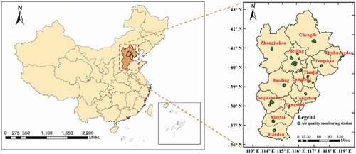
In recent years, China has paid more attention to air pollution control and air pollution control has begun to have impacts. However, air pollution problems in the Beijing-Tianjin-Hebei (BTH) region are still severe, and air pollution management has a long way to go. (https://energyandcleanair.org/wp/wp-content/uploads/2020/01/CREA-brief-China2019-Zh.pdf). The BTH area (113°E–120°E and 36°N–43°N) covers 13 cities with a population of 110 million and an area of 218,000 km². The BTH region is a rapidly developing area in China where frequent air pollution occurs.

In this case study, two types of datasets were used to validate the performance of the proposed model as follows: air pollution monitoring data and meteorological data. Air pollution monitoring data were obtained from the National City Air Quality Real-time Publishing Platform (http://106.37.208.233:20035/). This dataset contains hourly air pollution data (PM_2.5, PM₁₀, O₃, CO, SO₂, and NO₂) from 62 air quality monitoring stations in the BTH area, China, collected from 1 January 2016, to 31 December 2019. Meteorological data were obtained from China Meteorological Data Service Center (CMDC: http://data.cma.cn/en). This dataset contains daily meteorological data in the BTH area matched to each air quality monitoring station through inverse distance-weighted spatial interpolation, and the time scale is consistent with that of air pollution data. Meteorological data included precipitation (PRE), air pressure (PRS), relative humidity (RHU), sunshine (SSD), temperature (TEM), and wind direction and speed (WIN). Figure 1 shows the study area and distribution of 62 air quality monitoring stations (green circles). Table S1 lists the statistical characteristics of selected data.

Figure 1. The location of the study area (BTH) and distribution of air quality monitoring stations over the BTH area

2.2 Problem definition

This study aims to predict the average air pollution concentration in the next 24 h based on historical air pollution data from all stations in the BTH region. In our study, we proposed a GT-LSTM model that integrates the spatial and temporal dependencies of air pollutants. Thus, the prediction results could be achieved by the proposed GT-LSTM model, denoted as F(·), which is based on graph G and feature matrix X as shown in equation (2)(2) $X=\left[X_p,X_m,X_o\right]=\left[\begin{array}{ccccccc}{x}_{p,t-r}^1& \cdots & x_{p,t}^1& x_{m,t+1}^1& \cdots & x_{m,t+f}^1& x_o^1\\ x_{p,t-r}^2& \cdots & x_{p,t}^2& x_{m,t+1}^2& \cdots & x_{m,t+f}^2& x_o^2\\ ⋮& \ddots & ⋮& ⋮& \ddots & ⋮& ⋮\\ x_{p,t-r}^n& \cdots & x_{p,t}^n& x_{m,t+1}^n& \cdots & x_{m,t+f}^n& x_o^n\end{array}\right]$(2) , including historical air pollution data of all stations n with an interval of r denoted as X_p, meteorological data of the predicted period f denoted as X_m, and other feature data including one-hot encoding of time data (season and month data) denoted as X_o. It’s worth noting that since what we obtained is daily meteorological data, we matched the daily meteorological data to the predicted period (t + 1→t + f). Thus, the prediction problem of air pollution is framed as

(1) $Y=F\left(X;G\right)$(1)

(2) $X=\left[X_p,X_m,X_o\right]=\left[\begin{array}{ccccccc}{x}_{p,t-r}^1& \cdots & x_{p,t}^1& x_{m,t+1}^1& \cdots & x_{m,t+f}^1& x_o^1\\ x_{p,t-r}^2& \cdots & x_{p,t}^2& x_{m,t+1}^2& \cdots & x_{m,t+f}^2& x_o^2\\ ⋮& \ddots & ⋮& ⋮& \ddots & ⋮& ⋮\\ x_{p,t-r}^n& \cdots & x_{p,t}^n& x_{m,t+1}^n& \cdots & x_{m,t+f}^n& x_o^n\end{array}\right]$(2)

2.3 Spatial dependency modeling

2.3.1 Graph construction

Air pollution has apparent regional pollution transmission effects. In other words, there are significant spatial correlations among the air quality monitoring stations. In our study, a graph $G=\left(V,E\right)$with self-loops was constructed to capture spatial correlations among air quality monitoring stations, where V is the set of nodes representing air quality monitoring stations, and E is the set of edges, including self-loops denoting potential interactions among stations. The self-loops (as seen in Figure 1S) show that the future changes in air pollution concentration at each monitoring station will be self-affected by its historical monitoring values, which describe the local accumulation process of air pollutants. The links between any two different nodes indicate that the air pollution monitoring values of a single station are often affected by pollutants near stations in a certain area. Therefore, we constrain the links through:

(3) $e_{i,j}=\left\{\begin{array}{c}exist\\ none\end{array}\right.\begin{array}{c}if{d}_{i,j}\le 200km\\ otherwise\end{array}$(3)

where $e_{i,j}$represents the edge between node i and node j, and$d_{i,j}$represents the geographic distance between nodes i and j. We set $d_{i,j}$= 200 km as the distance threshold. Table S2 shows the edge numbers of all the stations in each city over the BTH area.

In addition, a spatial-weighted adjacency matrix $W\in {\mathbb{R}}^{{ }^{n\times n}}$was built to compute the spatial correlations of the nodes, where n is the number of nodes. The matrix W is defined by calculating the spatial correlation coefficients. The values of the matrix W at the diagonal position (the matrix value of the self-loop) were defined as the correlation coefficients of each station before and after a specific time interval r. The other values of matrix W were characterized by calculating the correlation coefficients among the different nodes. Before calculating the correlation coefficients, each station’s air pollution historical data need to be normalized using the min-max scaling method. The correlation coefficients $r_{i,j}$ were calculated as following formula (4), which were applied to define the matrix W as following formula (5).

(4) $r_{i,j}=\left\{\begin{array}{c}r\left({\tilde{x}}_{p,t}^i,{\tilde{x}}_{p,t}^j\right)=\frac{{\sum }_t^T\left({\tilde{x}}_{p,t}^i-{\bar{x}}_i\right)\left({\tilde{x}}_{p,t}^j-{\bar{x}}_j\right)}{{\sum }_t^T{\left({\tilde{x}}_{p,t}^i-{\bar{x}}_i\right)}^2{\sum }_t^T{\left({\tilde{x}}_{p,t}^j-{\bar{x}}_j\right)}^2}ifi\ne j\\ r\left({\tilde{x}}_{p,t}^i,{\tilde{x}}_{p,t+r}^i\right)=\frac{{\sum }_t^{T-r}\left({\tilde{x}}_{p,t}^i-{\bar{x}}_i\right)\left({\tilde{x}}_{p,t+r}^i-{\bar{x}}_i\right)}{{\sum }_t^{T-r}{\left({\tilde{x}}_{p,t}^i-{\bar{x}}_i\right)}^2{\sum }_t^{T-r}{\left({\tilde{x}}_{p,t+r}^i-{\bar{x}}_i\right)}^2}ifi\ne j\end{array}\right.$(4)

(5) $w_{i,j}=\left\{\begin{array}{c}{\tilde{r}}_{i,j}\\ 0\end{array}\right.\begin{array}{c}if\left(i,j\right)isanedge\\ otherwise\end{array}$(5)

where${\tilde{x}}_{p,t}^i$ and ${\tilde{x}}_{p,t}^j$represent the normalized air pollution data during time interval T at node i and node j, respectively. ${\tilde{x}}_{p,t+r}^i$ represents the normalized air pollution data after ${\tilde{x}}_{p,t}^i$with the time interval r at node i. ${\bar{x}}_i$ and ${\bar{x}}_j$ represent the mean values of ${\tilde{x}}_{p,t}^i$and ${\tilde{x}}_{p,t}^j$, respectively. ${\tilde{r}}_{i,j}$ represents the normalized correlation coefficients $r_{i,j}$.

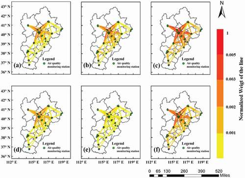
The spatial weighted adjacency matrix reveals the spatial correlations among different stations and the temporal correlations of the sites themselves. In this way, the values with large weights often appear on the adjacent sides where the pollution transmission of two adjacent points is relatively close. Figure 2 shows the spatial distribution of the edge weights of the different pollutants in the BTH area. From the perspective of air pollutants, we can see that the edge weight values of PM_2.5, PM₁₀, O₃, and NO₂ were higher, while the edge weight values of SO₂ were lower. This indicates that the formation of local pollutants, especially O₃, PM₁₀, and NO₂, which have a high degree of spatial correlation, is primarily affected by the transmission of air pollution from other places. From the perspective of spatial distribution, there are higher edge weight values in the central cities of the BTH area, such as Beijing, Tianjin, and Baoding, while the edge cities have lower weight values.

Figure 2. The spatial distribution of the edge weights of different pollutants in the BTH area: (a)PM_2.5, (b)PM₁₀, (c)O₃, (d)CO, (e)SO₂, and (f)NO_2.

2.3.2 Graph convolution

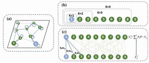
We adopted a K-order graph convolution method to simulate the horizontal transmission of pollutants by gathering neighborhood information and updating node information to capture the spatial correlations of the different air pollutants. This method is based on the idea of parameter sharing by performing graph convolution operations on the weighted adjacency matrix of the graph, which can reduce the computational complexity. $X_p^K$ represents the output of each pollutant at all nodes on the graph after the K-order graph convolution operation. The graph convolution denotes the multiplication of the K-order polynomial graph filter$g_{\theta }$with the input X_p of each pollutant at all nodes. The order K represents the convolution kernel size, which can leverage the information of each node and its K-order neighbor nodes on the graph to capture sufficient spatial correlations. Different nodes capture spatial dependence heterogeneity based on the weighted adjacency matrix W and the trainable shared parameters θ₀, …, θ_K-1 in the graph convolution. The study showed that a higher K value indicates a larger spatial dependence scale for modeling, but will confuse redundant spatial-related information and add noise to the model, increasing the computational costs and reducing the performance of the model. The study proved that the prediction results performed better when K was 2 (Zhang et al. 2020b). Thus, the size of the convolution kernel K was set to two in this study. As shown in Figure 3, we focused on the first node. When K = 1, it means performing a graph convolution operation with itself, that is,$X_p^0={\theta }_0{W}^0{X}_p$, and when K = 2, it means performing a graph convolution operation with the nodes directly connected to it, including nodes 2 and 3. After the 2-order graph convolution operation, $X_p^1={\sum }_k^1{\theta }_k{W}^{{ }_k}{X}_p$, the formulation of the K-order graph convolution can be defined as follows:

(6) $X_p^K=W_{\ast G}{X}_p=g_{\theta }\left(W\right)X={\theta }_0{W}^0{X}_p+{\theta }_1{W}^1{X}_p+\cdots +{\theta }_{K-1}{W}^{{ }_{K-1}}{X}_p={\sum }_k^{K-1}{\theta }_k{W}^{{ }_k}{X}_p$(6)

where $X_p^K=(x_p^{K,1},\dots ,x_p^{K,n})$denotes the output of the K-order graph convolution at each node, W^K−1 is the spatial weighted adjacency matrix W of the K-order graph convolution, and W⁰ is the diagonal matrix. $\theta =({\theta }_0,\dots ,{\theta }_{K-1})$ is a vector of trainable shared parameters.

Figure 3. Illustration of the K-order graph convolution: (a) weighted graph; (b) K-order domain representation of the node 1; (c) graph convolution operator of K = 2

2.4 Temporal dependency modeling

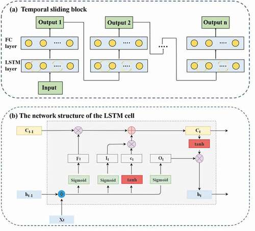
Air pollution data are long-term series data with a high degree of temporal correlation. The LSTM network is a typical model that can capture the temporal dependence of time-series data. LSTM controls the transmission of cyclic information through a gating mechanism and state variables. A detailed introduction to the LSTM network is provided in the Supplementary Information. However, as the prediction time increases, the time interval between prediction and training increases, making it difficult for the model to maintain a high degree of temporal correlations. The temporal sliding strategy was used to expand the long-term prediction task. It is based on the combination of a multi-layer bidirectional LSTM and a fully connected (FC) layer to capture the long-term change. The study proved the method of temporal sliding prediction could improve the conventional LSTM model’s prediction ability in long-term series by integrating the optimal time lag r = 12 h. (Mao et al. 2021). The strategy of temporal sliding prediction and the network structure of the LSTM cell are shown in Figure 4.

Figure 4. (a) Temporal sliding block; (b) The network structure of the LSTM cell

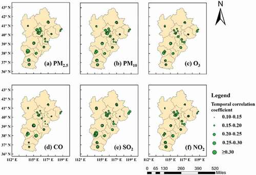
To evaluate the temporal dependency of different air pollutants, the maximal information coefficient (MIC) was used to calculate the temporal correlations between the time lag r = 12 h and the predicted period f = 24 h for different air pollutants. The MIC is used to measure the linear or non-linear correlation strength between two variables (Kinney and Atwal 2014; Reshef et al. 2011), and the formula is as follows:

(7) $\begin{array}{rl}& MIC\left(x;y\right)=\underset{a\ast b<B}{max}\frac{I\left(x;y\right)}{lo{g}_{2}min\left(a;b\right)}\\ & C_i=\frac{{\sum }_{t_1=0}^{t_1=r}{\sum }_{t2=0}^{t_2=f}MIC\left(x_{p,t_1}^i;x_{p,t_2}^i\right)}{r\times f}\end{array}$(7)

where x and y represent the data before and after the time lag, respectively; a and b are the number of grids in the x and y directions, respectively, and B is a variable, which is generally set to the 0.6th power of the amount of data (Kinney and Atwal 2014). C_i is the mean MIC value of each time lag value and the predicted point at each time point.

Figure 5 shows the temporal correlation coefficients of the 62 air quality monitoring stations over the BTH area for different air pollutants. From the perspective of air pollutants, it can be seen from Figure 5 that there are stronger temporal correlations of PM_2.5, PM₁₀ and other pollutants. From the perspective of spatial distribution, the stations in southern cities such as Shijiazhuang and Xingtai, have stronger temporal correlations than those in northern cities, revealing that pollutants in the south of the region tend to accumulate locally.

Figure 5. The temporal autocorrelation coefficients of 62 selected stations for different air pollutants

2.5 GT-LSTM model

To capture the spatiotemporal dependencies of different air pollutants, our study established GT-LSTM models for all air pollutants by integrating graph convolutional networks and LSTM networks with a temporal sliding strategy. The proposed model can conduct collaborative training on the monitoring data of the study area to predict the average pollutant concentration of each monitoring station in the next 24 h. A schematic proposed GT-LSTM model is illustrated in Figure 6. Taking the significant spatiotemporal correlations of air pollutants into account, the historical time lag r air pollution data were used as graph signals at each monitoring station. As can be seen in Figure 6, the GT-LSTM model consists of two main components: spatial dependency modeling and temporal dependency modeling based on the strategy with temporal sliding.

Figure 6. The framework of the proposed GT-LSTM model

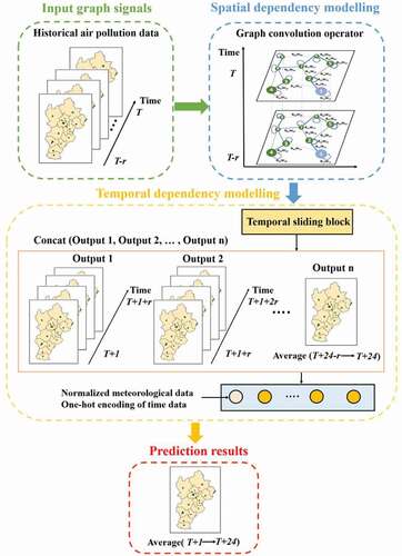
Graph convolution is utilized to transmit and aggregate information from neighbors to extract spatial characteristics. To ensure that both temporal and spatial features are extracted simultaneously, we embedded the graph convolution operator into temporal dependency modeling. This operation changes the input of information transmission in the LSTM network. The information transmission formulas in the LSTM network with the graph convolution operator are as follows:

(8) $\begin{array}{rl}& F_t=\sigma \left(W_f\left[W_{\ast G}{X}_{p,t},h_{t-1}\right]+b_f\right)\\ & I_t=\sigma \left(W_i\left[W_{\ast G}{X}_{p,t},h_{t-1}\right]+b_i\right)\\ & O_t=\sigma \left(W_o\left[W_{\ast G}{X}_{p,t},h_{t-1}\right]+b_o\right)\\ & c_t=tanh\left(W_c\left[W_{\ast G}{X}_{p,t},h_{t-1}\right]+b_c\right)\\ & C_t=F_t\odot C_{t-1}+I_t\odot c_t\\ & h_t=O_t\odot tanh\left(C_t\right)\end{array}$(8)

where, $W_f$, $W_i$, $W_o$and $W_c$are the weight matrices for the input vectors with the graph convolution operator $W_{\ast G}{X}_{p,t}$ at the current moment, $b_f$, $b_i$, $b_o$, and $b_c$ are the bias vectors. F_t, I_t, and O_t are the forget, input, and output gates, respectively, which determine whether passing a new input, blocking the current state, and letting the current state affect the output at each time step. C_t-1 and h_t-1 represent the internal and external states of the last moment, and $W_{\ast G}{X}_{p,t}$, C_t, and h_t represent the input, internal, and external states of the current moment, respectively. c_t represents the candidate state. $\sigma$and tanh are activation functions that can cause nonlinearity in the model. $\odot$represents the element-wise multiplication of matrix.

In temporal dependency modeling, we adopted the strategy of temporal sliding prediction to improve the accuracy of long-term prediction. The temporal sliding prediction is performed at the same time lag r to form a temporal sliding block until the air pollution in the next 24 h is predicted. According to the configured time lag value r, the predicted future 24-hour time period is divided into q = 24/r intervals, which is the number of temporal sliding predictions. The results of each temporal sliding prediction were the inputs for the next prediction. Taking r = 12 as an example, two temporal sliding processes will be performed, generating two-time period forecast results (Output 1: 1–12 h, Output 2: 13–24 h). In addition, to reduce the accumulation of errors in the temporal sliding prediction, the final output is the mean value. We depict the process of the temporal sliding prediction model, denoted as L(·), to obtain the predicted values of each period in the future in Equation (9)(9) $\begin{array}{rl}& \left[x_{p,t+1},\cdots ,x_{p,t+1+r}\right]=L\left(x_{p,t-r},\cdots ,x_{p,t};G\left(V,E\right)\right)\\ & \left[x_{p,t+1+r},\cdots ,x_{p,t+1+2r}\right]=L\left(x_{p,t+1},\cdots ,x_{p,t+1+r};G\left(V,E\right)\right)\\ & =L\left(L\left(x_{p,t-r},\cdots ,x_{p,t};G\left(V,E\right)\right)\right)\\ & \cdots \\ & {\bar{x}}_{\left[p;t+24-r,t+24\right]}==\underset{qtimes}{\underbrace{L\left(\cdots L\left(L\left(x_{p,t-r},\cdots ,x_{p,t};G\left(V,E\right)\right)\right)\right)}}\end{array}$(9) . We obtained output 1($x_{p,t+1},\cdots ,x_{p,t+1+r}$), output 2($x_{p,t+1+r},\cdots ,x_{p,t+1+2r}$), …, output n(${\bar{x}}_{\left[p;t+24-r,t+24\right]}$) by iterating the q times of the graph operations and temporal sliding.

(9) $\begin{array}{rl}& \left[x_{p,t+1},\cdots ,x_{p,t+1+r}\right]=L\left(x_{p,t-r},\cdots ,x_{p,t};G\left(V,E\right)\right)\\ & \left[x_{p,t+1+r},\cdots ,x_{p,t+1+2r}\right]=L\left(x_{p,t+1},\cdots ,x_{p,t+1+r};G\left(V,E\right)\right)\\ & =L\left(L\left(x_{p,t-r},\cdots ,x_{p,t};G\left(V,E\right)\right)\right)\\ & \cdots \\ & {\bar{x}}_{\left[p;t+24-r,t+24\right]}==\underset{qtimes}{\underbrace{L\left(\cdots L\left(L\left(x_{p,t-r},\cdots ,x_{p,t};G\left(V,E\right)\right)\right)\right)}}\end{array}$(9)

Studies have demonstrated that meteorological and temporal characteristics affect the changing trend of air pollution (Li et al. 2017; Zhang et al. 2018). After the predicted results (Output 1, Output 2, …, Output n) are concatenated, we added the normalized meteorological data of future predicted periods and one-hot encoding of time data as supplementary data for the GT-LSTM model. The spatiotemporal eigenvectors of the previous process and auxiliary data are integrated into the fully connected layer, which can obtain the predicted results of each monitoring station in the next 24 h. The prediction result can be expressed using the proposed GT-LSTM model as follows:

(10) $Y=F\left(x_{p,t+1},\cdots ,{\bar{x}}_{\left[p;t+24-r,t+24\right]};X_m;X_o\right)$(10)

3. Experiments and results

3.1 Experimental settings

We established GT-LSTM models for all air pollutants based on 35,064 h of air pollutant data from 1 January 2016, to 31 December 2019, divided into 60% for the training set, 20% for the validation set, and the remaining 20% for the test set. The time series filling method and neighboring station filling method were used to deal with missing values according to the significant spatiotemporal correlations of air pollution concentration. In the proposed model, the convolution kernel K was set to 2, and the time lag r was set to 12.

To verify the performance of the GT-LSTM model, we compared the following models established as baselines for all air pollutants:

• MLR refers to the method of establishing a forecast model through a period of historical monitoring value and future forecast value correlation analysis. The models were established based on the stations with the best network architecture.

• LSTM, which is suitable for time series forecasting, only captures temporal correlations and ignores the influence of external factors such as meteorological factors.

• LSTME (Li et al. 2017) considers the influences of meteorological and temporal characteristics based on LSTM and adds these data to the auxiliary inputs of the model.

• TS-LSTME (Mao et al. 2021) uses a highly temporally correlated delay for temporal sliding prediction, which can achieve higher accuracy and stability in long-term prediction and adds auxiliary data (meteorological data and temporal data) into the model. However, this model does not fully consider the spatial correlations among air quality monitoring stations.

• GC-LSTM (Qi et al. 2019) combines graph convolutional and LSTM networks to model the spatiotemporal dependencies of air pollution to predict future changes. Compared with our proposed model, the model only used the reciprocal of the distance as the weighted matrix in the spatial modeling and failed to capture the extended temporal dependence features effectively in the temporal modeling, which resulted in not digging into the spatiotemporal correlations of pollution data. Moreover, the model uses a spectral domain graph convolution method that is different from the GT-LSTM model.

The inputs of the models were based on LSTM (LSTM, LSTME, TS-LSTME, and GC-LSTM). The time lag r, the number of nodes in each neuron layer structure, and the output structures were the same as the settings of the proposed GT-LSTM model. Four metrics were used as accuracy indicators to evaluate the prediction performance of the GT-LSTM model: root mean square error (RMSE), mean absolute error (MAE), coefficient of determination (R²), and normalized root mean square error (NRMSE). These indicators can be formulated as follows:

(11) $\begin{array}{rl}& RMSE=\sqrt{\frac{1}{N}\sum _{i=1}^N{\left(P_i-O_i\right)}^2}\\ & MAE=\frac{1}{N}\sum _{i=1}^N\left|P_i-O_i\right|\\ & R^2=1-{\frac{{\sum }_{i=1}^N\left(P_i-O_i\right)}{{\sum }_{i=1}^N{\left({\bar{O}}_i-O_i\right)}^2}}^2\\ & NRMSE=\frac{RMSE}{O_{max}-O_{min}}\end{array}$(11)

where O_i is the observed air pollutant concentration, $\overline{O_i}$ is the average observed air pollutant concentration, O_max is the observed maximum value of air pollutant concentration, O_min is the observed minimum value of air pollutant concentration, P_i is the predicted air pollutant concentration, and N is the number of test samples.

3.2 Performance of the proposed GT-LSTM model

To evaluate the performance of various air quality predictions, we applied the proposed model to predict mean PM_2.5, PM₁₀, O₃, CO, SO₂, and NO₂ concentrations in the next 24 h. As shown in Table 1, the evaluation results show that the MAE values of PM_2.5, PM₁₀, O₃, CO, SO₂, and NO₂ prediction tasks accounted for 18%, 24%, 19%, 27%, 27%, and 29% of the mean value of the test set, respectively. The R² results were all above 0.76, and the NRMSE results were below 7.25%, which indicates that the proposed models show good performance in the prediction of different pollutants. It can be observed from Figure 7 the predicted values by the GT-LSTM model were generally consistent with the observed values of various air pollutants. There is a phenomenon that the slopes of the regression equation are often lower than 1.0, and the intercepts are above 0.0, indicating that there were more underestimated data samples than overestimated data samples. According to the R² value of each air pollutant, they were sorted as PM_2.5, O₃, NO₂, PM₁₀, SO₂, and CO. As we can see, the models for predicting PM_2.5, O₃, NO₂, and PM₁₀ obtained higher slope values of regression equations (0.90, 0.87, 0.81, and 0.80, respectively) and could capture more explanatory variables compared to the models for predicting CO and SO₂ (0.75 and 0.77, respectively). Referring to the above analysis of the spatiotemporal correlations of different pollutants (Figures 2 and 5), the results demonstrate the influences of spatiotemporal dependency on modeling.

Figure 7. Correlations between predicted and observed concentrations by the GT-LSTM model for various air pollutants on the test set (the number of data points is 434,744). The solid red lines and the dashed blue lines are the regression line and y = x reference line, respectively

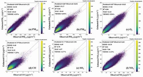
Table 1. Evaluations of the GT-LSTM models for the six air pollution predicting tasks

Air pollution	RMSE	MAE	R^2	NRMSE (%)	Mean
PM2.5	14.34	10.16	0.89	4.51	55.45
PM10	29.27	20.69	0.80	6.04	83.87
O3	17.04	12.42	0.86	5.54	63.25
CO	0.40	0.28	0.76	7.25	1.02
SO2	6.69	4.57	0.78	6.57	16.45
NO2	10.34	7.86	0.81	6.23	40.04

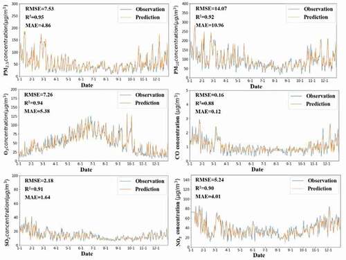
To explore the prediction performances of the GT-LSTM model more intuitively, we compared the daily average monitoring concentration of pollutants in the BTH region with the daily average concentration predicted by the model. The test set with a time interval of 12–23 hours every day was selected to predict the daily average pollutant concentration in the following day. As shown in Figure 8, the R² values of various pollutants ranged from 0.88 to 0.95, and the predicted values of each pollutant were consistent with the temporal changing trend of the observed values. Moreover, GT-LSTM can capture peaks in multiple periods, and these peaks often require more attention to help in the joint prevention and control of air pollutants. The results show that the proposed model can promptly track changes in pollutants, and its prediction is close to observed values, indicating that the proposed framework is effective and promising for various air pollutant forecasting in practice.

Figure 8. Comparison of temporal distribution between predicted and observed daily mean six air pollutants by GT-LSTM models for the BTH area from 1 January 2019 to 31 December 2019

3.3 Comparison of experiments

The comparison results of the different models are presented in Table 2. In general, for PM_2.5, PM₁₀, O₃, CO, SO₂, and NO₂ prediction tasks, the four indicators of the proposed model are better than those of the five baselines. The R² values and NRMSE values of the GT-LSTM models range from 0.76 to 0.89% and from 4.55% to 7.25%, respectively. It can be seen that the MLR models (R²: 0.23–0.32, NRMSE: 12.23–14.31%) perform the worst in prediction compared to the other models. The results indicate that the simple machine learning method finds it difficult to handle time-series data and simulate the changing air pollution trend, whereas the models based on deep learning frameworks (LSTM, LSTME, TS-LSTME, GC-LSTM, and GC-LSTM) perform well. To evaluate the ability of our GT-LSTM model to capture temporal dependency, we compared it with the LSTM, LSTME, and TS-LSTME models. The results show that the GT-LSTM and the TS-LSTME (R²: 0.65–0.78, NRMSE 6.35–9.23%) models performed better than the LSTM (R²: 0.40–0.53, NRMSE: 8.44–11.05%) and LSTME models (R²: 0.43–0.57, NRMSE: 7.96–10.50%), which demonstrates that the models with temporal sliding prediction can maintain higher temporal correlations. The proposed models outperformed the TS-LSTME models, which emphasizes the importance of modeling spatial dependency. Moreover, the GC-LSTM models (R²: 0.71–0.81, NRMSE: 6.27–8.88%) were inferior to the GT-LSTM models. There are several reasons for this phenomenon: (1) In spatial modeling, the spatial adjacency weighting matrix established in this study was more effective in capturing the domain information of the stations. Additionally, compared with the Chebyshev method used by GC-LSTM, we applied the graph convolution network method to help reduce the complexity of calculation and improve the accuracy to a certain extent when applied to the prediction of large areas. (2) In temporal modeling, GC-LSTM models utilize a simple LSTM structure, while the strategy with temporal sliding is applied to the GT-LSTM models, indicating the superiority of the strategy with temporal sliding in the model application. It is worth noting that the results show that the accuracy of GC-LSTM is relatively higher than that of the TS-LSTME models owing to the consideration of spatial correlation. However, in the SO₂ prediction task, owing to the strong temporal dependence of SO₂ and weaker spatial transmission, the prediction performance of TS-LSTME models is better than that of GC-LSTM, which further highlights the significant impacts of the spatiotemporal correlations of pollutants on modeling.

Table 2. Overall performances of different models on all air pollutants

Air pollution	Metric	MLR	LSTM	LSTME	TS-LSTME	GC-LSTM	GT-LSTM
PM2.5	RMSE	38.87	26.62	25.09	20.04	19.79	14.34
	MAE	29.51	19.43	18.17	13.81	13.12	10.16
	R^2	0.32	0.53	0.57	0.78	0.80	0.89
	NRMSE	12.23%	8.44%	7.96%	6.35%	6.27%	4.55%
PM10	RMSE	60.51	46.38	43.16	33.12	32.21	29.27
	MAE	41.27	30.92	29.47	22.71	22.65	20.69
	R^2	0.27	0.49	0.52	0.76	0.76	0.80
	NRMSE	12.48%	9.57%	8.91%	6.83%	6.65%	6.04%
O3	RMSE	42.63	32.11	30.52	23.36	20.97	17.04
	MAE	34.69	23.96	20.37	16.21	14.62	12.42
	R^2	0.26	0.43	0.49	0.76	0.81	0.86
	NRMSE	13.86%	10.43%	9.79%	7.59%	6.81%	5.54%
CO	RMSE	0.79	0.61	0.58	0.51	0.49	0.4
	MAE	0.54	0.43	0.4	0.34	0.3	0.28
	R^2	0.23	0.40	0.43	0.65	0.71	0.76
	NRMSE	14.31%	11.05%	10.50%	9.23%	8.88%	7.25%
SO2	RMSE	13.69	10.03	9.26	7.1	8.69	6.69
	MAE	9.47	6.85	6.54	4.95	5.12	4.57
	R^2	0.24	0.46	0.5	0.75	0.71	0.78
	NRMSE	13.44%	9.84%	9.10%	6.97%	8.53%	6.57%
NO2	RMSE	21.97	16.97	15.86	13.55	12.23	10.34
	MAE	15.32	13.02	12.44	10.34	9.12	7.86
	R^2	0.25	0.42	0.46	0.73	0.77	0.81
	NRMSE	13.23%	10.22%	9.55%	8.16%	7.37%	6.23%

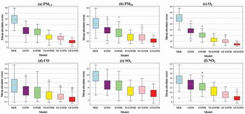
Compared with other models, the RMSE values of the GT-LSTM models in various air pollutant prediction tasks were reduced by approximately 123.7%, 66.5%, 56.4%, 25.8%, and 23.6%, respectively, on average. The MAE values were 127.3%, 68.7%, 55.7%, 24.5%, and 16.9%. Figure 9 displays the boxplots of MAE values produced by different models for various pollutants, which can visually show the dispersion of prediction errors. We can clearly see that the proposed models have the smallest outlier distribution of the MAE values. In addition, the GT-LSTM models produced fewer errors and exhibited better stability and robustness compared with the baselines.

Figure 9. Boxplots of MAE results for different models

4. Discussion

4.1 Spatial error distribution

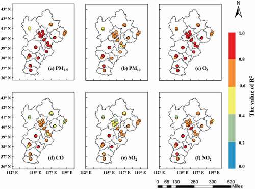
To further evaluate the performance of the proposed GT-LSTM model in space, we analyzed the spatial error distribution of the stations for different air pollutants. According to Figure 10, the accuracy values of the stations in the southern and central regions of the BTH area are generally higher than those of the northern fringe cities. The R² values of the northern fringe cities such as Zhangjiakou, Chengde, and Qinhuangdao are between 0.3 and 0.8, and the cities in the central and southern regions are between 0.4 and 1.0. This error distribution can be explained by analyzing the spatiotemporal correlations of air pollutants in various cities, as shown in Figures 2 and 5. For cities in the central region, such as Beijing, Tianjin, and Baoding, more information about their neighbors was contained for spatial modeling, which can better help simulate the transmission of air pollution between different cities, while in cities of the peripheral region, the spatially adjacent neighbors are not entirely included, resulting in lower accuracy. However, air pollutants in cities in the southern area, such as Xingtai, Handan, Shijiazhuang, and Hengshui tend to accumulate more locally, creating stronger temporal correlations than northern fringe cities. Relevant studies also show that the multi-year average wind speed in the BTH region is generally high in the north and low in the south, with the northwest wind as the prevailing wind direction in the north and southerly wind as the prevailing wind direction in the south (Wang, Zhao et al. 2019b; Zhang et al. 2018). Meteorological characteristics also lead to differences in the spatial distribution of the spatiotemporal correlations of air pollutants, leading to spatial differences in the model’s prediction ability. Thus, the above results suggest the importance of fully considering spatiotemporal dependency to simulate the diffusion and local accumulation of air pollution.

Figure 10. Spatial distribution of the R² values for various air pollutants at each station in the BTH area

4.2 Limitations and future work

In terms of methodology, our study proposed a model (GT-LSTM) for predicting air pollution with respect to spatiotemporal correlations. The proposed model could help better simulate the temporal and spatial changes of pollutants by allowing efficient spatiotemporal dependencies, which could assist in controlling environmental pollution and reducing the cost of air pollution treatment, thereby improving the efficiency of air pollution control. The RMSE values of the PM_2.5, PM₁₀, O₃, CO, SO₂ and NO₂ forecast models constructed in our study were 14.34 μg/m³, 29.27 μg/m³, 17.04 μg/m³, 0.40 mg/m³, 6.69 μg/m³, and 10.34 μg/m³, respectively. According to the China Ambient Air Quality Standards (CAAQS) (http://www.mee.gov.cn/ywgz/fgbz/bz/bzwb/dqhjbh/dqhjzlbz/201203/W020120410330232398521.pdf) implemented in 2016, as shown in Table S3, the limits of the 24-hour average concentrations of PM_2.5, PM₁₀, CO, SO₂, NO₂ on level2 are 75 μg/m³, 150 μg/m³, 4 mg/m³, 150 μg/m³ and 80 μg/m³, and the maximum eight-hour ozone limit is 160 μg/m³. The comparison shows that the errors of the model are within the acceptable error range, which demonstrates that the model can be applied to different air pollutant prediction tasks and has a broad scientific outlook on the atmospheric environment. However, there are still some improvements required for the proposed model in future works. First, the slopes of the regression equations are often less than 1.0, indicating that more values are underestimated than overestimated. This will greatly affect the early warning and control of air pollution. Future research will analyze this phenomenon from the perspective of data distribution, and methods such as data enhancement should be used to improve the performance of the model. Second, especially in extreme weather or abnormal conditions, it is difficult for the model to capture future temporal and spatial changes in air pollution. In future research, we will focus on air pollution in these conditions to establish a more robust prediction model. Third, air pollution change is a dynamic and complex system, and factors such as geographical barriers and anthropogenic factors play important roles in air pollution forecasting. Therefore, in future research, we will utilize more data and build dynamic models based on deep learning to improve air pollution spatiotemporal prediction accuracy and apply it to realize longer time-series predictions of various pollution on larger scales, such as the national scale.

5. Conclusions

Air pollution is mainly caused by local accumulation and transmission from other places, which are both closely related to the spatiotemporal correlations of air pollution. How to effectively build a model suitable for various types of air pollution to simulate the accumulation and diffusion to enhance the prediction accuracy is a critical issue in this field. In this study, we developed and presented a hybrid deep learning framework for spatiotemporal modeling to predict various air pollutants leveraging graph convolution and long short-term networks. We established transmission networks for various air pollutants with each node on the graph as a monitoring station and the connectable edges as the connection relationship. In this study, graph convolutional networks were used to obtain spatial dependence by performing graph convolution operations on the adjacencies of various pollutants, which simulated the diffusion of air pollutants. The LSTM networks and the self-loops of each point on the network were used to capture the dynamic changes in the node attributes, which simulated the accumulation of air pollutants. To maintain high temporal correlations in long-term predictions, a strategy with temporal sliding was applied to the LSTM networks. By configuring the above structures, the proposed GT-LSTM model deeply explored the spatiotemporal correlations of various air pollutants, simulating the future temporal and spatial changes in air pollution accurately. GT-LSTM was evaluated on real data sets, including six pollutants (PM_2.5, PM₁₀, O₃, CO, SO₂, and NO₂) in the BTH region and compared with other state-of-the-art models. The results show that our proposed model realized more accurate and stable predictions, indicating the success of our approach. We also discussed the spatial error distributions of various air pollutants. The results showed that the distribution of errors in space correspond to the distribution of spatiotemporal correlation strength to a certain extent, revealing the importance of spatiotemporal dependence modeling for pollutant prediction. This study provides new concepts and methods for air pollution forecasting, which will help relevant departments to prevent and control air pollution in advance more accurately and in a more targeted manner. The prediction results of the proposed GT-LSTM model can provide directional support for urban construction, industrial planning, traffic organization, residents’ travel decisions, and environmental emission reduction decisions.

Highlights

A hybrid integrated model is proposed for various pollutants predictions.

The proposed model could capture high spatiotemporal characteristics of different pollutants.

The proposed model achieved higher accuracy and stability in various pollution predictions.

Acknowledgements

This study was supported by the National Natural Science Foundation of China (41971368) and National Key R&D Program of China [Grant Numbers: 2017YFA0604404).

Disclosure statement

The authors declare no competing interests

Data availability statement

The data and codes that support the findings of this study are available on request from the corresponding author.

Additional information

Funding

This work was supported by the National Key R&D Program of China [2017YFA0604404]; the National Natural Science Foundation of China [41971368].

References

- A., V., G. P, R. V., and K. P. S. 2018. “DeepAirNet: Applying Recurrent Networks for Air Quality Prediction.” Procedia Computer Science 132: 1394–1403. doi:https://doi.org/10.1016/j.procs.2018.05.068.
- Agirre-Basurko, E., G. Ibarra-Berastegi, and I. Madariaga. 2006. “Regression and Multilayer Perceptron-based Models to Forecast Hourly O3 and NO2 Levels in the Bilbao Area.” Environmental Modelling and Software 21 (4): 430–446. doi:https://doi.org/10.1016/j.envsoft.2004.07.008.
- Akinwumiju, A. S., T. Ajisafe, and A. A. Adelodun. 2021. “Airborne Particulate Matter Pollution in Akure Metro City, Southwestern Nigeria, West Africa: Attribution and Meteorological Influence.” J Geovis Spat Anal 5 (1): 11. doi:https://doi.org/10.1007/s41651-021-00079-6.
- Althuwaynee, O. F., A.-L. Balogun, and W. A. Madhoun. 2020. “Air Pollution Hazard Assessment Using Decision Tree Algorithms and Bivariate Probability Cluster Polar Function: Evaluating Inter-correlation Clusters of PM10 and Other Air Pollutants.” GIScience & Remote Sensing 57 (2): 207–226. doi:https://doi.org/10.1080/15481603.2020.1712064.
- Arhami, M., N. Kamali, and M. M. Rajabi. 2013. “Predicting Hourly Air Pollutant Levels Using Artificial Neural Networks Coupled with Uncertainty Analysis by Monte Carlo Simulations.” Environ Science Pollut Res 20 (7): 4777–4789. doi:https://doi.org/10.1007/s11356-012-1451-6.
- Barzeghar, V., P. Sarbakhsh, M. S. Hassanvand, S. Faridi, and A. Gholampour. 2020. “Long-term Trend of Ambient Air PM10, PM2.5, And O3 and Their Health Effects in Tabriz City, Iran, during 2006–2017.” Sustainable Cities and Society 54: 101988. doi:https://doi.org/10.1016/j.scs.2019.101988.
- Chen, D., N. Zhao, J. Lang, Y. Zhou, X. Wang, Y. Li, Y. Zhao, and X. Guo. 2018. “Contribution of Ship Emissions to the Concentration of PM2.5: A Comprehensive Study Using AIS Data and WRF/Chem Model in Bohai Rim Region, China.” Science of the Total Environment 610–611: 1476–1486. doi:https://doi.org/10.1016/j.scitotenv.2017.07.255.
- Filonchyk, M., V. Hurynovich, H. Yan, and S. Yang. 2020. “Atmospheric Pollution Assessment near Potential Source of Natural Aerosols in the South Gobi Desert Region, China.” GIScience & Remote Sensing 57 (2): 227–244. doi:https://doi.org/10.1080/15481603.2020.1715591.
- Franceschi, F., M. Cobo, and M. Figueredo. 2018. “Discovering Relationships and Forecasting PM10 and PM2.5 Concentrations in Bogotá, Colombia, Using Artificial Neural Networks, Principal Component Analysis, and K-means Clustering.” Atmospheric Pollution Research 9 (5): 912–922. doi:https://doi.org/10.1016/j.apr.2018.02.006.
- Friberg, M. D., X. Zhai, H. A. Holmes, H. H. Chang, M. J. Strickland, S. E. Sarnat, P. E. Tolbert, A. G. Russell, and J. A. Mulholland. 2016. “Method for Fusing Observational Data and Chemical Transport Model Simulations to Estimate Spatiotemporally Resolved Ambient Air Pollution.” Environmental Science & Technology 50 (7): 3695–3705. doi:https://doi.org/10.1021/acs.est.5b05134.
- Gariazzo, C., G. Carlino, C. Silibello, M. Renzi, S. Finardi, N. Pepe, P. Radice, et al. 2020. “A Multi-city Air Pollution Population Exposure Study: Combined Use of Chemical-transport and random-Forest Models with Dynamic Population Data.” Science of the Total Environment 724: 138102. doi:https://doi.org/10.1016/j.scitotenv.2020.138102.
- Geng, G., Q. Zhang, R. V. Martin, A. van Donkelaar, H. Huo, H. Che, J. Lin, and K. He. 2015. “Estimating Long-term PM2.5 Concentrations in China Using Satellite-based Aerosol Optical Depth and a Chemical Transport Model.” Remote Sensing of Environment 166: 262–270. doi:https://doi.org/10.1016/j.rse.2015.05.016.
- Hochreiter, S., and J. Schmidhuber. 1997. “Long Short-Term Memory.” Neural Computation 9 (8): 1735–1780. doi:https://doi.org/10.1162/neco.1997.9.8.1735.
- Hu, J., B. Ostro, H. Zhang, Q. Ying, and M. J. Kleeman. 2019. “Using Chemical Transport Model Predictions to Improve Exposure Assessment of PM2.5 Constituents.” Environmental Science 6(8): 456–461. doi:https://doi.org/10.1021/acs.estlett.9b00396.
- Ibarra-Berastegi, G., A. Elias, A. Barona, J. Saenz, A. Ezcurra, and J. Diaz de Argandoña. 2008. “From Diagnosis to Prognosis for Forecasting Air Pollution Using Neural Networks: Air Pollution Monitoring in Bilbao.” Environmental Modelling and Software 23 (5): 622–637. doi:https://doi.org/10.1016/j.envsoft.2007.09.003.
- Jeong, J. I., and R. J. Park. 2018. “Efficacy of Dust Aerosol Forecasts for East Asia Using the Adjoint of GEOS-Chem with Ground-based Observations.” Environmental Pollution 234: 885–893. doi:https://doi.org/10.1016/j.envpol.2017.12.025.
- Juhos, I., L. Makra, and B. Tóth. 2009. “The Behaviour of the Multi-layer Perceptron and the Support Vector Regression Learning Methods in the Prediction of NO and NO2 Concentrations in Szeged, Hungary.” Neural Comput & Applic 18 (2): 193–205. doi:https://doi.org/10.1007/s00521-007-0171-1.
- Kinney, J. B., and G. S. Atwal. 2014. “Equitability, Mutual Information, and the Maximal Information Coefficient.” Proc Natl Acad Sci USA 111 (9): 3354–3359. doi:https://doi.org/10.1073/pnas.1309933111.
- Lee, H.-M., R. J. Park, D. K. Henze, S. Lee, C. Shim, H.-J. Shin, K.-J. Moon, and J.-H. Woo. 2017. “PM2.5 Source Attribution for Seoul in May from 2009 to 2013 Using GEOS-Chem and Its Adjoint Model.” Environmental Pollution 221: 377–384. doi:https://doi.org/10.1016/j.envpol.2016.11.088.
- Leng, X., J. Wang, H. Ji, Q. Wang, H. Li, X. Qian, F. Li, and M. Yang. 2017. “Prediction of Size-fractionated Airborne Particle-bound Metals Using MLR, BP-ANN and SVM Analyses.” Chemosphere 180: 513–522. doi:https://doi.org/10.1016/j.chemosphere.2017.04.015.
- Li, X., L. Peng, X. Yao, S. Cui, Y. Hu, C. You, and T. Chi. 2017. “Long Short-term Memory Neural Network for Air Pollutant Concentration Predictions: Method Development and Evaluation.” Environmental Pollution 231: 997–1004. doi:https://doi.org/10.1016/j.envpol.2017.08.114.
- Lightstone, S. D., F. Moshary, and B. Gross. 2017. Comparing CMAQ Forecasts with a Neural Network Forecast Model for PM2.5 In New York16.
- Liu, S., S. Hua, K. Wang, P. Qiu, H. Liu, B. Wu, P. Shao, et al. 2018. “Spatial-temporal Variation Characteristics of Air Pollution in Henan of China: Localized Emission Inventory, WRF/Chem Simulations and Potential Source Contribution Analysis.” Science of the Total Environment 624: 396–406. doi:https://doi.org/10.1016/j.scitotenv.2017.12.102.
- Ma, J., Y. Ding, J. C. P. Cheng, F. Jiang, V. J. L. Gan, and Z. Xu. 2020. “A Lag-FLSTM Deep Learning Network Based on Bayesian Optimization for Multi-sequential-variant PM2.5 Prediction.” Sustainable Cities and Society 60: 102237. doi:https://doi.org/10.1016/j.scs.2020.102237.
- Ma, X., T. Sha, J. Wang, H. Jia, and R. Tian. 2018. “Investigating Impact of Emission Inventories on PM2.5 Simulations over North China Plain by WRF-Chem.” Atmospheric Environment 195: 125–140. doi:https://doi.org/10.1016/j.atmosenv.2018.09.058.
- Mao, W., W. Wang, L. Jiao, S. Zhao, and A. Liu. 2021. “Modeling Air Quality Prediction Using a Deep Learning Approach: Method Optimization and Evaluation.” Sustainable Cities and Society 65: 102567. doi:https://doi.org/10.1016/j.scs.2020.102567.
- Martins, N. R., and G. Carrilho da Graça. 2018. “Impact of PM2.5 In Indoor Urban Environments: A Review.” Sustainable Cities and Society 42: 259–275. doi:https://doi.org/10.1016/j.scs.2018.07.011.
- Ortolani, C., and M. Vitale. 2016. “The Importance of Local Scale for Assessing, Monitoring and Predicting of Air Quality in Urban Areas.” Sustainable Cities and Society 26: 150–160. doi:https://doi.org/10.1016/j.scs.2016.06.001.
- Paschalidou, A. K., S. Karakitsios, S. Kleanthous, and P. A. Kassomenos. 2011. “Forecasting Hourly PM10 Concentration in Cyprus through Artificial Neural Networks and Multiple Regression Models: Implications to Local Environmental Management.” Environ Science Pollut Res 18 (2): 316–327. doi:https://doi.org/10.1007/s11356-010-0375-2.
- Peng, H., A. R. Lima, A. Teakles, J. Jin, A. J. Cannon, and W. W. Hsieh. 2017. “Evaluating Hourly Air Quality Forecasting in Canada with Nonlinear Updatable Machine Learning Methods.” Air Quality, Atmosphere, & Health 10 (2): 195–211. doi:https://doi.org/10.1007/s11869-016-0414-3.
- Qi, Y., Q. Li, H. Karimian, and D. Liu. 2019. “A Hybrid Model for Spatiotemporal Forecasting of PM2.5 Based on Graph Convolutional Neural Network and Long Short-term Memory.” Science of the Total Environment 664: 1–10. doi:https://doi.org/10.1016/j.scitotenv.2019.01.333.
- Reshef, D. N., Y. A. Reshef, H. K. Finucane, S. R. Grossman, G. McVean, P. J. Turnbaugh, E. S. Lander, M. Mitzenmacher, and P. C. Sabeti. 2011. “Detecting Novel Associations in Large Data Sets.” Science 334 (6062): 1518–1524. doi:https://doi.org/10.1126/science.1205438.
- Rubal, K. D. 2018. “Evolving Differential Evolution Method with Random Forest for Prediction of Air Pollution.” Procedia Computer Science 132: 824–833. doi:https://doi.org/10.1016/j.procs.2018.05.094.
- Unnithan, S. L. K., and L. Gnanappazham. 2020. “Spatiotemporal Mixed Effects Modeling for the Estimation of PM2.5 From MODIS AOD over the Indian Subcontinent.” GIScience & Remote Sensing 57 (2): 159–173. doi:https://doi.org/10.1080/15481603.2020.1712101.
- Vlachogianni, A., P. Kassomenos, A. Karppinen, S. Karakitsios, and J. Kukkonen. 2011. “Evaluation of a Multiple Regression Model for the Forecasting of the Concentrations of NOx and PM10 in Athens and Helsinki.” Science of the Total Environment 409 (8): 1559–1571. doi:https://doi.org/10.1016/j.scitotenv.2010.12.040.
- Wang, J., and G. Song. 2018. “A Deep Spatial-Temporal Ensemble Model for Air Quality Prediction.” Neurocomputing 314: 198–206. doi:https://doi.org/10.1016/j.neucom.2018.06.049.
- Wang, L., S. Wang, L. Zhang, Y. Wang, Y. Zhang, C. Nielsen, M. B. McElroy, and J. Hao. 2014. “Source Apportionment of Atmospheric Mercury Pollution in China Using the GEOS-Chem Model.” Environmental Pollution 190: 166–175. doi:https://doi.org/10.1016/j.envpol.2014.03.011.
- Wang, P., X. Qiao, and H. Zhang. 2020. “Modeling PM2.5 And O3 with Aerosol Feedbacks Using WRF/Chem over the Sichuan Basin, Southwestern China.” Chemosphere 254: 126735. doi:https://doi.org/10.1016/j.chemosphere.2020.126735.
- Wang, Q., Q. Zeng, J. Tao, L. Sun, L. Zhang, T. Gu, Z. Wang, and L. Chen. 2019a. “Estimating PM2.5 Concentrations Based on MODIS AOD and NAQPMS Data over Beijing–Tianjin–Hebei.” Sensors 19 (5): 1207. doi:https://doi.org/10.3390/s19051207.
- Wang, S., Y. Li, J. Zhang, Q. Meng, L. Meng, and F. Gao, 2020. “PM2.5-GNN: A Domain Knowledge Enhanced Graph Neural Network For PM2.5 Forecasting.” arXiv:2002.12898 [cs, eess].
- Wang, W., S. Zhao, L. Jiao, M. Taylor, B. Zhang, G. Xu, and H. Hou. 2019b. “Estimation of PM2.5 Concentrations in China Using a Spatial Back Propagation Neural Network.” Scientific Reports 9 (1): 13788. doi:https://doi.org/10.1038/s41598-019-50177-1.
- Wen, C., S. Liu, X. Yao, L. Peng, X. Li, Y. Hu, and T. Chi. 2019. “A Novel Spatiotemporal Convolutional Long Short-term Neural Network for Air Pollution Prediction.” Science of the Total Environment 654: 1091–1099. doi:https://doi.org/10.1016/j.scitotenv.2018.11.086.
- Woody, M. C., H.-W. Wong, J. J. West, and S. Arunachalam. 2016. “Multiscale Predictions of Aviation-attributable PM2.5 For U.S. Airports Modeled Using CMAQ with Plume-in-grid and an Aircraft-specific 1-D Emission Model.” Atmospheric Environment 147: 384–394. doi:https://doi.org/10.1016/j.atmosenv.2016.10.016.
- Xiao, Q., H. H. Chang, G. Geng, and Y. Liu. 2018. “An Ensemble Machine-Learning Model to Predict Historical PM 2.5 Concentrations in China from Satellite Data.” Science Technol 52 (22): 13260–13269. doi:https://doi.org/10.1021/acs.est.8b02917.
- Yang, X., Q. Wu, R. Zhao, H. Cheng, H. He, Q. Ma, L. Wang, and H. Luo. 2019. “New Method for Evaluating Winter Air Quality: PM2.5 Assessment Using Community Multi-Scale Air Quality Modeling (CMAQ) in Xi’an.” Atmospheric Environment 211: 18–28. doi:https://doi.org/10.1016/j.atmosenv.2019.04.019.
- Yang, Z., and J. Wang. 2017. “A New Air Quality Monitoring and Early Warning System: Air Quality Assessment and Air Pollutant Concentration Prediction.” Environmental Research 158: 105–117. doi:https://doi.org/10.1016/j.envres.2017.06.002.
- Zhan, Y., and J. Kim. 2020. “Editorial: Special Issue on “Air Quality Monitoring, Assessment, & Forecasting Using GIScience and Remote Sensing.” GIScience & Remote Sensing 57 (2): 157–158. doi:https://doi.org/10.1080/15481603.2020.1726625.
- Zhang, B., L. Jiao, G. Xu, S. Zhao, X. Tang, Y. Zhou, and C. Gong. 2018. “Influences of Wind and Precipitation on Different-sized Particulate Matter Concentrations (PM2.5, PM10, PM2.5–10).” Meteorol Atmos Phys 130 (3): 383–392. doi:https://doi.org/10.1007/s00703-017-0526-9.
- Zhang, K., J. Thé, G. Xie, and H. Yu. 2020a. “Multi-step Ahead Forecasting of Regional Air Quality Using Spatial-temporal Deep Neural Networks: A Case Study of Huaihai Economic Zone.” Journal of Cleaner Production 277: 123231. doi:https://doi.org/10.1016/j.jclepro.2020.123231.
- Zhang, Y., T. Cheng, Y. Ren, and K. Xie. 2020b. “A Novel Residual Graph Convolution Deep Learning Model for Short-term Network-based Traffic Forecasting.” International Journal of Geographical Information Science 34 (5): 969–995. doi:https://doi.org/10.1080/13658816.2019.1697879.
- Zhao, J., F. Deng, Y. Cai, and J. Chen. 2019. “Long Short-term Memory - Fully Connected (LSTM-FC) Neural Network for PM2.5.” Concentration Prediction. Chemosphere 220: 486–492. doi:https://doi.org/10.1016/j.chemosphere.2018.12.128.
- Zhao, R., L. Zhan, M. Yao, and L. Yang. 2020. “A Geographically Weighted Regression Model Augmented by Geodetector Analysis and Principal Component Analysis for the Spatial Distribution of PM2.5.” Sustainable Cities and Society 56: 102106. doi:https://doi.org/10.1016/j.scs.2020.102106.
- Zhu, S., X. Lian, L. Wei, J. Che, X. Shen, L. Yang, X. Qiu, et al. 2018. “PM2.5 Forecasting Using SVR with PSOGSA Algorithm Based on CEEMD, GRNN and GCA considering Meteorological Factors.” Atmospheric Environment 183: 20–32. doi:https://doi.org/10.1016/j.atmosenv.2018.04.004.