A comparison of three ways to assemble wall-to-wall maps from distribution models of vegetation types

ABSTRACT

Distribution modeling methods are used to provide occurrence probability surfaces for modeled targets. While most often used for modeling species, distribution modeling methods can also be applied to vegetation types. However, surfaces provided by distribution modeling need to be transformed into classified wall-to-wall maps of vegetation types to be useful for practical purposes, such as nature management and environmental planning. The paper compares the performance of three methods for assembling predictions for multiple vegetation types, modeled individually, into a wall-to-wall map. The authors used grid-cell based probability surfaces from distribution models of 31 vegetation types to test the three assembly methods. The first, a probability-based method, selected for each grid cell the vegetation type with the highest predicted probability of occurrence in that cell. The second, a performance-based method, assigned the vegetation types, ordered from high to low model performance, to a fraction of the grid cells given by the vegetation type’s prevalence in the study area. The third, a prevalence-based method, differed from the performance-based method by assigning vegetation types in the order from low to high prevalence. Thus the assembly methods worked in two principally different ways: the probability-based method assigned vegetation types to grid cells in a cell-by-cell manner, and both the performance-based method and prevalence-based method assigned them in a type-by-type manner. All methods were evaluated by use of reference data collected in the field, more or less independently of the data used to parameterize the vegetation-type models. Quantity, allocation, and total disagreement, as well as proportional dissimilarity metrics, were used for evaluation of assembly methods. Overlay analysis showed 38.1% agreement between all three assembly methods. The probability-based method had the lowest total disagreement with, and proportional dissimilarity from, the reference datasets, but the differences between the three methods were small. The three assembly methods differed strongly with respect to the distribution of the total disagreement on its quantity and allocation components: the cell-by-cell assignment method strongly favored allocation disagreement and the type-by-type methods strongly favored quantity disagreement. The probability-based method best reproduced the general pattern of variation across the study area, but at the cost of many rare vegetation types, which were left out of the assembled map. By contrast, the prevalence-based and performance-based methods represented vegetation types in accordance with nationwide area statistics. The results show that maps of vegetation types with wall-to-wall coverage can be assembled from individual distribution models with a quality acceptable for indicative purposes, but all the three tested methods currently also have shortcomings. The results also indicate specific points in the methodology for map assembly that may be improved.

KEYWORDS:

• Area frame survey
• assembly strategies
• distribution modeling
• spatial probabilities
• vegetation mapping
• vegetation types

Introduction

The partitioning of a landscape into a few predefined land cover types is a well-studied topic in remote sensing. Land cover maps of large areas can be successfully derived through the use of image classification of satellite data in combination with reference data from the field surveys (“ground truths” (Feranec et al. 2016)). However, remote sensing-based approaches have so far not proven able to identify functional vegetation types defined by community structure and species composition (Myers-Smith et al. 2020). Vegetation maps are valuable tools for ecological research, conservation planning, and management of natural resources. Today, categorical vegetation maps with types defined by the species composition are largely based on field surveys, such as the British National Vegetation Classification (NVC) survey (Mucina et al. 1993; Rodwell 2018), the European Vegetation Survey (EVS) (MNHN-EEA 2014), the LUCAS survey (Eurostat 2003), and the Norwegian AR18x18 survey (Strand 2013). In contrast to remote sensing-based categories defined by physiognomy and separated by spectral signatures (Assal, Anderson, and Sibold 2015), field-based vegetation-type mapping is time-consuming and expensive (Ullerud, Bryn, and Klanderud 2016). Accordingly, only a fraction of the Earth’s surface has been mapped by field survey methods (Alexander and Millington 2000), and alternative and more cost-efficient ways to produce wall-to-wall maps of vegetation types are needed to cover large areas.

Species distribution modeling is a well-established method for relating targets, such as species, to a set of predictors (Guisan, Thuiller, and Zimmermann 2017). During recent decades, distribution modeling has emerged as one of the most important applied tools for biodiversity modeling (Araújo et al. 2019), typically for summarization and ecological explanation of spatial distribution patterns, and for projection of species distributions into the future. Spatial predictions are typically represented as prediction surfaces (i.e. maps) of occurrence probabilities across a study area at a given resolution. Nevertheless, distribution models for single species are of limited value for applied purposes that require information about the distribution of higher levels of either biodiversity or ecodiversity (Halvorsen et al. 2020), such as vegetation or land-cover types. Compared with single-species distribution modeling, the development of methodologies for modeling these higher levels is still lagging behind (Ovaskainen and Abrego 2020) despite recent developments (D’Amen et al. 2017). Typically, the community level of organization is approached by assembling models of individual species in the vegetation rather than taking advantage of the fact that vegetation types are entities that, like species, can be recorded as present or absent at each specific point in space, and hence can be characterized by their geographic distribution, local abundance, and other properties used to characterize species (Simensen et al. 2020).

Many methods, such as logistic regression (Horvath et al. 2019) and classification trees (Dalle Fratte, Brusa, and Cerabolini 2019), have been used for modeling the distribution of individual vegetation types or habitat types. However, few studies have taken the logical next step of building a single-layered map of categorized units from predictions for each of those units (Cawsey, Austin, and Baker 2002; Mikolajczak et al. 2015; Jiménez-Alfaro et al. 2018) in accordance with the “predict first, assemble later” strategy for building community models from single-species models (Ferrier and Guisan 2006). Such a stepwise strategy for assembling individual-target prediction models into a model for a higher-level target may also be advantageous for several reasons relating to application. Distribution models assembled from individual vegetation-type models into a coarser thematic resolution such as plant functional types may, for instance, assist parameterization of dynamic vegetation models in earth system models (ESMs) (Horvath et al. 2021). The main aim of the present study is to compare three different approaches to the assembly of a wall-to-wall single-layered map of vegetation types for a large area based on individual distribution models of single vegetation types. Based on the results of the comparison, we aim to explain differences in the outcomes by the map assembly approaches and to discuss critical aspects of the methodology. We accomplish these aims by using terrestrial Norway as our study area, for which Horvath et al. (2019) obtained distribution models for 31 vegetation types. The performance of the three approaches is evaluated by the use of three field-based reference datasets, of which two were collected independently of the dataset used to parameterize the distribution models of the vegetation types.

Material and methods

Study area

The study area covered 291,360 km² and comprised the terrestrial ecosystems of Norway, excluding urban areas, agricultural land, lakes, glaciers, and persistent snow (Figure 1). These four land-cover types (hereafter referred to as “the four left-out AR50 categories,” (Heggem Mathisen, and Frydenlund 2019)), cover 0.7, 2.9, 0.7, and 5.5% of the total terrestrial area of Norway respectively (323,802 km²), and are excluded because their distinct and well-known geographic distribution, thus make modeling unnecessary. The study area spans latitudes from 57°57’N to 71°11ʹN, longitudes from 4°29ʹE to 31°10ʹE, and an altitudinal range from sea level to 2,469 m a.s.l. All seven bioclimatic temperature-related vegetation zones commonly recognized in northern Europe, from boreonemoral to high alpine, exist in Norway (Bakkestuen, Erikstad, and Halvorsen 2008). The wide range of climatic variation, high mineral and bedrock diversity (Ramberg et al. 2008), and extensive variation in landforms and hydrology (Simensen, Erikstad, and Halvorsen 2021) have resulted in a high diversity of ecosystem types (Halvorsen et al. 2020). Moreover, Norwegian ecosystems have a long history of use for domestic grazing, heath burning, reindeer husbandry, forestry, and industrial, urban, and recreational development (Almås et al. 2004).

Figure 1. The study area (dark gray) comprising the terrestrial area of Norway and excluding urban areas (red), agricultural lands orange), glaciers, permanent snow (cyan) and lakes (blue)

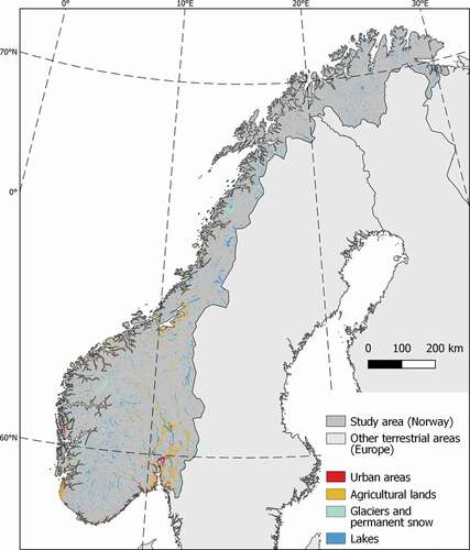
Figure 2. Area coverage of reference datasets AR18×18 (panel A left), AR9×9 (panel B center) and AR VEG (panel C right)

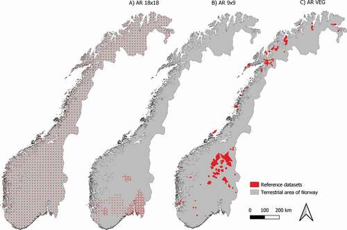
Figure 3. Flow diagram for the three methods used to assemble wall-to-wall vegetation maps from 31 vegetation-type probability surfaces. While the probability-based method assigns vegetation types to grid cells on a cell-by-cell basis, both the performance-based method and the prevalence-based method assign vegetation types to grid cells on a type-by-type basis

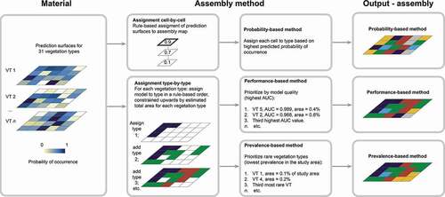
Figure 4. Wall-to-wall vegetation maps of Norway assembled from vegetation-type models by three different assembly methods: the probability-based method, the performance-based method, and the prevalence-based method. “The four left-out AR50 categories” represent land-cover types taken from AR 50 land-cover maps not subjected to modeling

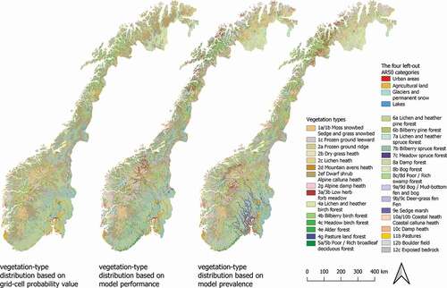
Figure 5. An area in southern central Norway (see blue box on location map), mapped at a scale of 1:25,000 by the vegetation mapping system used by NIBIO. (A) The AR VEG reference map for the area. (B–D) The three assembled maps, obtained by (B) the probability-based method, (C) the performance-based method, and (D) the prevalence-based method

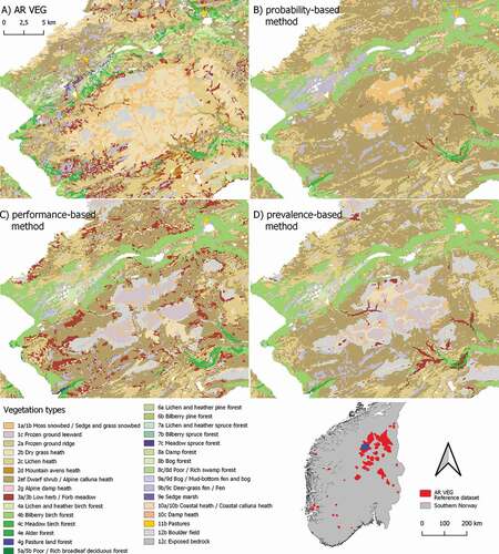
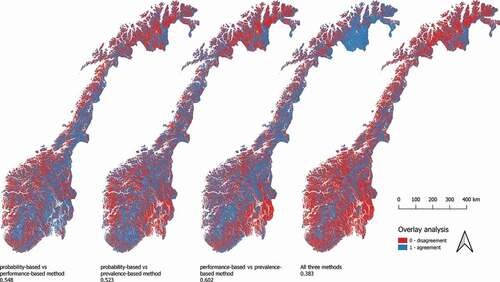
Figure 6. Geographic distribution of grid cells similarly and differently assigned to vegetation types by the three assembly methods, resulting from pairwise and three-way overlay analysis. Proportional agreement (as a fraction of 1) is given for all overlay maps

Data sets

Three datasets, compiled through vegetation mapping efforts, were used for this study as training and evaluation data for the assembled wall-to-wall maps of vegetation types. A vegetation map was provided for each plot, obtained for the same type system as used in this study (see Table 1).

Table 1. The 31 vegetation types used in this study and properties of the respective distribution models. The properties used for assigning vegetation types to grid cells by the three assembly methods are shown in the three rightmost columns: (i) maximum predicted probability of occurrence in any cell (relevant for the probability-based method); (ii) the AUC goodness-of-fit statistic for each distribution model (relevant for the performance-based method); and (iii) the estimated prevalence in the study area according to Bryn et al. (2018) (relevant for the prevalence-based method)

Code	Vegetation type	(i) Predicted probability of occurrence	(ii) Model performance (AUC)	(iii) Prevalence (% of area)
1a/1b	Moss snowbed/Sedge and grass snowbed	0.916	0.904	4.5
1c	Frozen ground, leeward	0.873	0.966	1.5
2a	Frozen ground, ridge	0.965	0.988	0.6
2b	Dry grass heath	0.941	0.957	0.5
2c	Lichen heath	0.999	0.851	6.0
2d	Mountain avens heath	0.272	0.884	0.9
2e/2f	Dwarf shrub/Alpine Calluna heath	0.565	0.796	13.9
2g	Alpine damp heath	0.735	0.985	1.9
3a/3b	Low herb/Forb meadow	0.914	0.783	2.6
4a	Lichen and heather birch forest	0.995	0.746	3.7
4b	Bilberry birch forest	0.081	0.708	6.2
4c	Meadow birch forest	0.905	0.788	3.4
4e	Alder forest	0.466	0.821	0.4
4g	Pasture land forest	0.299	0.856	0.2
5a/5b	Poor/Rich broadleaf deciduous forest	0.834	0.989	0.4
6a	Lichen and heather pine forest	0.991	0.896	8.1
6b	Bilberry pine forest	0.614	0.888	1.2
7a	Lichen and heather spruce forest	0.025	0.671	1.2
7b	Bilberry spruce forest	0.452	0.880	6.9
7c	Meadow spruce forest	0.643	0.832	2.1
8a	Damp forest	0.326	0.952	1.0
8b	Bog forest	0.059	0.837	0.7
8c/8d	Poor/Rich swamp forest	0.067	0.676	2.2
9a/9d	Bog/Mud-bottom fen and bog	0.250	0.751	2.7
9b/9c	Deer-grass fen/Fen	0.656	0.708	6.1
9e	Sedge marsh	0.040	0.888	0.1
10a/10b	Coastal heath/Coastal Calluna heath	0.444	0.923	1.3
10c	Damp heath	0.083	0.894	0.7
11b	Pastures	0.190	0.679	0.9
12b	Boulder field	0.988	0.887	4.6
12c	Exposed bedrock	0.996	0.931	3.5

The AR18×18 dataset derived from the Norwegian area-frame survey of land cover and outfield land resources) (Figure 2(A)) consisted of 1,081 rectangular 600 × 1,500 m plots spaced in a regular grid measuring 18 km in the latitudinal and longitudinal directions (Bryn et al. 2018). The total area covered by the plots was 971.14 km² and thus provided area-representative information for the study area. However, parts of this dataset have previously been utilized in training of the individual vegetation models (also see the section “Material” below), and therefore cannot be considered fully independent of the modeling procedure.

The AR9×9 dataset (Figure 2(B)), a densified version of the AR18×18 dataset in selected parts of southern Norway, consisted of 236 plots in a grid with 9 km mesh width, superimposed on the AR18×18 grid by inserting plots along the west–east and/or south–north directions in a non-overlapping manner. Like AR18×18 plots, each plot covered 600 × 1,500 m and had an associated vegetation-type map. The total area covered by AR9×9 plots was 212 km² (ca. 0.07% of the total study area). Due to its limited spatial coverage, the dataset only included presence observations of 29 out of the 31 vegetation types (Frozen ground, ridge (2a) and Mountain avens heath (2d) were not present in the area covered by the AR9×9 dataset).

The AR VEG dataset (Figure 2(C)) consisted of vegetation-type maps resulting from a large number of vegetation mapping projects carried out between 1997 and 2015, mainly in eastern and coastal northern Norway. The dataset covered 8,663.75 km² (2.7% of the total study area). The area covered by AR VEG partly or fully overlapped 33 plots in the AR18×18 dataset (a total land area of 23.4 km²).

The AR18×18, AR9×9, and AR VEG datasets, which are collectively referred to as the reference datasets, vary in their fraction used to parameterize and evaluate the vegetation-type models obtained by Horvath et al. (2019) (also see the section “Material” below). While the AR9×9 dataset was collected fully independently of the data used to parameterize vegetation-type models, fractions of the AR VEG and the AR18×18 datasets (larger for the latter) were used to parameterize the vegetation-type models. Therefore, none of the three reference datasets complies fully with strict ideals for evaluation of distribution models, namely representativity of the variation in the study area and complete independence of the data used to parameterize the models that are evaluated (Halvorsen 2012). The advantages of the AR18×18 dataset are even coverage of the study area and near-optimal representativity, as illustrated by the Kendall’s rank correlation coefficient τ = 0.9676 (p < 0.0001, n = 31) between prevalences of vegetation types in the AR18×18 dataset and the dataset used to model vegetation types. The advantages of AR VEG and AR9×9 are near or full independence of the training data, but neither of these datasets is representative of the distribution of vegetation types within Norway, as shown by the Kendall’s rank correlation coefficients τ = 0.5228 and τ = 0.6804 (both p < 0.0001, n = 31) respectively, between prevalences in the respective datasets. The complementarity of the three reference datasets used in this study for assessment of assembled maps is further illustrated by the much higher quantity disagreement values (see the “Methods” section for explanation) for two of the map assembly methods – the performance-based method and the prevalence-based method with the AR9×9 and AR VEG – than with the AR18×18 reference map. This reflects the lack of representativity of the former maps for Norway as a whole. Therefore, we argue that the three reference datasets complement each other and together form a solid basis for assessment of the performance of map assembly methods. Furthermore, we argue that the large differences in map comparison metric values among the datasets highlight the importance of unbiased representativity of datasets used for evaluation of distribution models, in addition to independence of the data used for model parameterization (Halvorsen 2012; Norberg et al. 2019).

All reference datasets were obtained by following a vegetation mapping system used by NIBIO (Bryn et al. 2018), which was also used to obtain the vegetation-type models (Horvath et al. 2019). The AR18×18, AR9×9, and AR VEG datasets were converted to reference maps with the same format as the assembled maps by reclassification from 57 to 31 vegetation-type categories, rasterization to 100 × 100 m grid cells, and masking out the four left-out AR50 categories.

Material

The material for the present study consisted of distribution models for 31 vegetation types, obtained by Horvath et al. (2019) (Table 1) in the study area. The 31 modeled vegetation types make up a subset of the total of 57 land-cover and vegetation categories in the vegetation mapping system used by NIBIO (Bryn et al. 2018). The models were trained using presence-absence data from the AR18×18 dataset in such way that one randomly generated point was used from each vegetation-type polygon and used as presence observation for the vegetation type in question and as an absence observation for all other vegetation types.

Distribution models for each of the 31 vegetation types were obtained by applying generalized linear modeling (“logistic regression”) to 116 predictor variables, either recorded at a resolution of 100 × 100 m or adapted to that grid-cell size by resampling or rasterization from vector formats (see Appendix 1). The predictors for the individual distribution models fall into categories of geological data (capturing variation in bedrock and quaternary deposits), topographic data (derived from a digital elevation model), climatic data (mean and extreme values for temperature and precipitation, derived BIOCLIM variables and snow), and land-cover data (area-resource data at a scale of 1:50,000). Strongly intercorrelated variables (|τ| > 0.7) were omitted. Variables were selected by a forward stepwise selection procedure based on F tests of nested models. The final 31 models were evaluated by applying the AUC criterion to two fully independent evaluation datasets, AR9×9 and AR VEG. AUC (the area under the receiver operator characteristic curve) is a threshold-independent measure of model performance commonly used for evaluation of distribution models (Fielding and Bell 1997). Because presence-absence data were used to parameterize the vegetation-type models, model predictions were interpreted as probability surfaces for each vegetation type (see Horvath et al. 2019 for further details and access to data).

Assembly of vegetation maps with wall-to-wall coverage

Three different approaches were used to assemble seamless vegetation maps from the 31 vegetation-type probability surfaces by assigning to each grid cell one and only one vegetation type to each grid cell. Therefore, the resulting maps did not contain any gaps or overlaps.

As a first step in the assembly process, the 31 vegetation-type probability surfaces were ordered in approach-specific ways (Figure 3). Thereafter, for each approach, one vegetation type was assigned to each grid cell in the study area by an approach-specific, rule-based procedure whereby priority was given to: (1) the vegetation type with the highest predicted probability of occurrence in each cell; (2) the vegetation type with the best-performing distribution model; and (3) the vegetation type with the lowest prevalence in the study area. After completion of the assembly process, the four left-out AR50 categories were added to the three maps for visual purposes.

With the first assembly method, hereafter referred to as the probability-based method, vegetation types were assigned to grid cells on a cell-to-cell basis, for each cell, selecting the vegetation type with the highest predicted probability of occurrence in that cell.

With the second and third assembly methods, vegetation types were assigned to grid cells on a type-by-type basis. In the case of the performance-based method, vegetation types were assigned to grid cells in order of decreasing value of AUC of the respective distribution models (values are tabulated in column (ii) in Table 1). Each vegetation type j was assigned to the number, n_j, of grid cells prescribed by the vegetation type’s prevalence (frequency of occurrence) reported in the national area statistics (column (iii) in Table 1 ; cf. Bryn et al. 2018). Thus, the assignment procedure started with the vegetation type with the highest AUC, namely Poor/rich broadleaf deciduous forest (5ab), which was assigned to 146,100 out of a total of 28,714,394 grid cells (= 0.4%) ranked 1–146,100 by predicted probabilities for that vegetation type. These grid cells were thereafter considered as “occupied.” Subsequently, the vegetation type with the second-highest model AUC, Frozen ground, ridge – 2a, was assigned to the 181,000 “unoccupied” cells ranked highest by predicted probabilities for that vegetation type. This procedure was repeated in an iterative manner for 27 of the 31 vegetation types (i.e. all except the four vegetation types with lowest model AUC: Lichen and heather birch forest – 4b, Lichen and heather spruce forest – 7a, Poor/rich swamp forest – 8c/8d, and Pastures – 11b). A total of 10.3% of the grid cells in the study area then remained unoccupied. Models for the four vegetation types differed from all other models as they contained one binary predictor only and therefore provided binary predictions, for example for Pastures (11b) values of 0.1896 and 0.0065 (Horvath et al. 2019). The four vegetation types (hereafter referred to as “the four vegetation types with binary predictions”) were assigned to the remaining “unoccupied” cells by, for each cell, assigning the one of the four vegetation types with the highest predicted probability of occurrence in that cell.

With the prevalence-based method, vegetation types were assigned to grid cells by the same iteration procedure as described above for the performance-based method, but in order of decreasing prevalence (i.e. rarity; see column (iii) in Table 1), as given by Bryn et al. (2018). The vegetation types with the lowest prevalence, Sedge marsh (9e), was assigned first. The most common vegetation type, Dwarf shrub/Alpine Calluna heath (2e/2f), was assigned last among these 27 vegetation types. The four vegetation types with binary predictions were assigned to the 10.3% of grid cells remaining unoccupied after the other 27 vegetation types had been assigned, using the procedure described for the performance-based method.

The three tested methods differ in several respects. Whereas the probability-based method only uses information from the assembled surfaces, making it easily applicable to other areas and types without additional information, the two type-by-type methods utilize the additional information about area statistics of the study area, which is thus required for the method to be used at different sites. While the first method is known from the literature (Cawsey, Austin, and Baker 2002; Mikolajczak et al. 2015), the latter two methods are, to our knowledge, novel approaches to map assembly.

Comparison of assembled maps

Overlay analysis

The maps resulting from the application of the three assembly methods were compared by simple overlay analysis. The fractional agreement – the fraction of grid cells to which the same vegetation type was assigned by either two compared maps (i.e. A∩B, A∩C and B∩C) or by all three maps (A∩B∩C) – was calculated.

Analysis of proportional dissimilarities from the AR18×18 dataset

Proportional dissimilarity (Czekanowski 1909), which is often, incorrectly, referred to as the Bray-Curtis index (for an explanation see Yoshioka 2008), was used as a spatially non-explicit measure of the fractional deviation of each assembled map from the vegetation maps of the AR18×18 dataset. For each AR18×18 plot k (k = 1, …, 1081), we first obtained a vegetation-type profile (i.e. a vector V_k of proportions z_kj for each of 32 categories (j = 1, …, 32) in the set of 90 grid cells of size 100 × 100 m. Elements j = 1, …, 31 of vector V_k represent the 31 vegetation types addressed in this study, while grid cells representing one of the 18 out of the 57 vegetation types in the vegetation mapping system used by NIBIO excluded from the present study were collectively assigned to one category represented as the 32nd vector element. The vectors V_k were used as references for plot-wise comparisons with the corresponding profile vectors V_sk = {z_skj} for each of the three assembled maps s (s = 1, …, 3, corresponding to the probability-based method, the performance-based method, and the prevalence-based method, respectively). Proportional dissimilarities d_sk were calculated between pairs of profile vectors V_sk and V_k, separately for each AR18×18 plot k and assembled map s. Proportional dissimilarity is the Manhattan measure standardized by division by the sum of the pairwise sums of variable values (here proportions z_kj). As the sum of the elements of each profile vector is one, the index reduces to

$d_{sk}=1-\hspace{0.17em}\sum _{j=1}^{32}\mathrm{m}\mathrm{i}\mathrm{n}\left(z_{skj},z_{kj}\right)$

For all assembled maps, the proportional dissimilarity with AR18×18 varied from a minimum of 0 (full agreement) to a maximum of 1 (full disagreement).

Evaluation methods

One 31 × 31 confusion matrix M_st was generated for each of the nine combinations of three assembled maps s (s = 1, …, 3, corresponding to the probability-based method, the performance-based method and the prevalence-based method, respectively) and three reference maps t (t = 1, …, 3, corresponding to AR18×18, AR9×9, and AR VEG, respectively). The row vectors of confusion matrix M_st represent vegetation-type categories in assembled map s, whereas the columns represent vegetation types in reference map t. Accordingly, element n_stij of confusion matrix M_st is the number of grid cells categorized as vegetation type j (j = 1, …, 31) in reference map t that are assigned to vegetation type i (i = 1, …, 31) in assembled map s. Diagonal elements n_stjj (i = j = 1, …, 31) provide counts of grid cells assigned to the same vegetation type in assembled map s and reference map t, while off-diagonal elements (i ≠ j) are counts of misclassified cells (Rossiter 2004).

Following Pontius Jr and Millones (2011), Olofsson et al. (2014), and Nelson et al. (2021), we quantified two components of map accuracy separately. Quantity disagreement (QD) is the amount of difference between reference map s and assembled map t that is due to the less than perfect match in the proportions of the categories (Pontius Jr and Millones 2011). QD was quantified for each combination of s, t, and vegetation type j as the difference between the numbers of grid cells classified as j in reference map t (n_stj.) and the number of grid cells assigned to j in assembled map s (n_st.j). It should be noted that “.” in the equations indicates summation of all cells for the index in question:

(1) $Q{D}_{stj}=\left|n_{st.j}-n_{stj.}\right|$(1)

Allocation disagreement (AD) is the amount of difference between reference map t and assembled map s that is due to the less than perfect match in the spatial allocation of the categories, given the proportions of the categories in the reference and assembled maps (Pontius and Millones 2011). AD was quantified for each combination of s, t, and vegetation type j as:

(2) $D_{stj}=2\left[min(n_{st.j},n_{stj.}\right)-n_{stjj}]$(2)

QD and AD sum to the total disagreement (TD), which can be expressed as:

(3) $D_{stj}=\hspace{0.17em}Q{D}_{stj}+\hspace{0.17em}A{D}_{stj}=n_{st.j}+n_{stj.}-2n_{stjj}$(3)

The disagreement statistics are additive and can be summarized over all j for each combination of maps s and t to overall measures of disagreement. These are referred to as QD_st, AD_st, and TD_st, respectively. Because the sums of each of n_st.j and n_stj∙ over all vegetation types j equal the total number of grid cells N_t in reference map t, the overall total disagreement TD_st simplifies to

(4) $T{D}_{st}=\hspace{0.17em}{N}_t+N_t-2\sum _{j=1}^{31}{n}_{stjj}=2\left(N_t-\sum _{j=1}^{31}{n}_{stjj}\right)=\hspace{0.17em}\frac{2}{N_t}\left(1-\sum _{j=1}^{31}{p}_{stjj}\right)$(4)

where p_stjj is the proportion of grid cells in map t assigned to category j in both maps. The term $1-\sum _{j=1}^{31}{p}_{stjj}$ in expression (4) is the complement of the much used metric “overall proportional agreement” (Landis and Koch 1977), or “intraclass correlation coefficient” (Monserud and Leemans 1992).

Because the numbers of grid cells differ among reference maps, we standardized all overall accuracy measures QD_st, AD_st, and TD_st by division with $\frac{2}{N_t}$ to bring them onto a common 0–1 scale on which the value 0 corresponds to complete agreement (all grid cells assigned to the same vegetation type in the two compared maps) and the value 1 corresponds to complete disagreement (no grid cell assigned to the same vegetation type). The standardized overall accuracy measures are denoted sQD, sAD, and sTD, respectively.

A fourth performance metric, proportion of lost vegetation types (LVT), was calculated as the fraction of vegetation types allocated to at least one grid cell in reference map t that was not assigned to any grid cell in assembled map s. The LVT metric quantifies the ability of the assembly methods to generate maps that maintain diversity at the vegetation-type level.

Software and packages

The assembly process and all statistical analysis were carried out in R (version 3.6.3) (R Core Team 2020). Spatial outputs were created in QGIS (version 3.14) (QGIS Development Team 2009). Raster and vector operations were carried out by using R packages “rgdal” (Rowlingson, Bivand, and Keitt 2019), “raster” (Hijmans 2019), and “sp” (Pebesma and Bivand 2005), while graphics are produced using the “ggplot2” package (Wickham 2016). Confusion matrices were obtained with the use of the “differ” package (Pontius Jr and Santacruz 2019), and the “vegan” package (Oksanen et al. 2019) was used to calculate proportional dissimilarity.

Results

Area statistics and geographic patterns of the three assembled maps

Visual inspection of the assembled maps for the entire study area (Figure 4) reveals that all models capture the general, broad-scale patterns by separating forest from alpine vegetation types. Inspection of grid-cells at smaller extents indicates that all assembly methods produce an overly simplified representation of the fine-scaled heterogeneous landscape compared with the reference maps (AR VEG; (Figure 5). In particular, this is the case for the map assembled by the probability-based method (Figure 5(b)), from which many of the vegetation types in the reference dataset are absent.

The probability-based method consistently overrepresented common vegetation types and underrepresented rare types (Table 2). The two most prevalent vegetation types, Dwarf shrub/Alpine Calluna heath (2e/2f) and Lichen and heather pine forest (6a), were assigned to 40.8% of the grid cells in the study area (25.2% and 15.6%, respectively), compared with a total of 22.0% (13.9% and 8.1%, respectively) in the AR18×18 reference dataset (e.g. Figure 5(B)).

Table 2. Area statistics for vegetation types for the three assembled maps using (ii) probability, (iii) performance and (iv) prevalence, compared with the area-representative statistics (i) for Norway (data source Bryn et al. 2018)

Vegetation type		(i) Norway		(ii) Probability-based method		(iii) Performance-based method		(iv) Prevalence-based method
Code	Vegetation type	Area (km2)	Area (%)	Area (km2)	Area (%)	Area (km2)	Area (%)	Area (km2)	Area (%)
1a/1b	Moss snowbed/Sedge and grass snowbed	14,613	4.5	21,227	6.6	14,613	4.5	14,613	4.5
1c	Frozen ground, leeward	4,908	1.5	735	0.2	4,908	1.5	4,908	1.5
2a	Frozen ground, ridge	1,810	0.6	297	0.1	1,810	0.6	1,810	0.6
2b	Dry grass heath	1,672	0.5	148	0.0	1,672	0.5	1,672	0.5
2c	Lichen heath	19,452	6.0	13,156	4.1	19,452	6.0	19,452	6.0
2d	Mountain avens heath	2,776	0.9	0	0.0	2,776	0.9	2,776	0.9
2e/2f	Dwarf shrub/Alpine Calluna heath	45,023	13.9	81,702	25.2	45,023	13.9	45,023	13.9
2g	Alpine damp heath	5,990	1.9	2,463	0.8	5,990	1.9	5,990	1.9
3a/3b	Low herb/Forb meadow	8,343	2.6	1,433	0.4	8,343	2.6	8,343	2.6
4a	Lichen and heather birch forest	11,905	3.7	15,317	4.7	11,905	3.7	11,905	3.7
4b	Bilberry birch forest	20,139	6.2	11,335	3.5	28,159	8.7	27,262	8.4
4c	Meadow birch forest	10,915	3.4	11,660	3.6	10,915	3.4	10,915	3.4
4e	Alder forest	1,117	0.4	69	0.0	1,117	0.3	1,117	0.3
4g	Pasture land forest	605	0.2	11	0.0	605	0.2	605	0.2
5a/5b	Poor/Rich broadleaf deciduous forest	1,461	0.4	282	0.1	1,461	0.5	1,461	0.5
6a	Lichen and heather pine forest	26,216	8.1	50,507	15.6	26,216	8.1	26,216	8.1
6b	Bilberry pine forest	3,996	1.2	384	0.1	3,996	1.2	3,996	1.2
7a	Lichen and heather spruce forest	3,938	1.2	0	0.0	0	0.0	0	0.0
7b	Bilberry spruce forest	22,439	6.9	28,237	8.7	22,439	6.9	22,439	6.9
7c	Meadow spruce forest	6,695	2.1	189	0.1	6,695	2.1	6,695	2.1
8a	Damp forest	3,382	1.0	347	0.1	3,382	1.0	3,382	1.0
8b	Bog forest	2,276	0.7	0	0.0	2,737	0.8	2,599	0.8
8c/8d	Poor/Rich swamp forest	7,221	2.2	11	0.0	69	0.0	142	0.0
9a/9d	Bog/Mud-bottom fen and bog	8,521	2.7	1,724	0.5	8,585	2.7	8,559	2.6
9b/9c	Deer-grass fen/Fen	19,988	6.1	25,919	8.0	19,988	6.2	19,988	6.2
9e	Sedge marsh	269	0.1	0	0.0	321	0.1	291	0.1
10a/10b	Coastal heath/Coastal Calluna heath	4,449	1.3	3,042	0.9	4,449	1.4	4,449	1.4
10c	Damp heath	2,370	0.7	0	0.0	2,370	0.7	2,370	0.7
11b	Pastures	2,805	0.9	3,565	1.1	1,082	0.3	2,100	0.6
12b	Boulder field	14,743	4.6	8,597	2.7	14,743	4.6	14,743	4.6
12c	Exposed bedrock	11,323	3.5	4,786	1.5	11,323	3.5	11,323	3.5
	SUM	291,360	90	287,144	88.7	287,144	88.7	287,144	88.7

A total of 7 of the 31 vegetation types were overrepresented by the probability-based method, all of which were among the 11 most prevalent vegetation types. The remaining 24 vegetation types were either clearly underrepresented by the probability-based method or were absent (5 vegetation types) from the assembled map (Table 2).

The map assembled by the probability-based method captured broad distributional patterns of common vegetation types in Norway, but the method did not detect distinct patterns of less common types, such as the zone of Poor/Rich broadleaf deciduous forest (5a/5b) along the coast of south-east Norway (Figure 4).

By definition, the performance-based method minimized quantity disagreement (i.e. recovered the prevalence) of all vegetation types. While the Poor/Rich broadleaf deciduous forest (5a/5b) was correctly assigned to coastal south-east Norway, other vegetation types were clearly incorrectly assigned to grid cells (e.g. Low herb/Forb meadows – 3a/3b; Figure 5(C).

The assignment of the four vegetation types with binary predictions was, unsurprisingly, burdened with considerable quantity disagreement. The most common vegetation type, Bilberry birch forest (4b), was assigned to 8.7% of the study area, compared with the prevalence of 6.2%; Table 2), while Poor/Rich swamp forest (8c/8d) was strongly underrepresented (covering only 69 km² instead of 2,276 km²), and Lichen and heather spruce forest (7a) was not represented on the map assembled by the performance-based method.

Like the performance-based method, the probability-based method minimized quantity disagreement by maintaining the prevalence of the 27 vegetation types with non-binary models. Visual inspection revealed considerable differences between the maps assembled by the two type-by-type methods (Figures 4 and 6). This is exemplified by the strong concentration of Meadow spruce forest (7c) in the major valleys in south-east Norway, and by the geographic shift in the distribution of Low herb/Forb meadows (3a/3b) (Figure 3).

Comparison of assembled maps

Overlay analysis

Overlay analyses revealed that the three assembly methods produced maps that were relatively similar in overall patterns, but far from identical in cell-by-cell comparison. The proportions of grid cells assigned to the same vegetation type (i.e. the overall proportional agreement calculated for pairs of assembled maps) were 0.602 for the performance-based method and the prevalence-based method, 0.548 for the probability-based method and the performance-based method, and 0.523 for the probability-based method and the prevalence-based method (Figure 6). The fraction of grid cells assigned identically by all three methods was 0.383, suggesting relatively high similarity between the three methods given the number of classes (n = 31). The geographic distribution of identical assignments varied somewhat between map pairs, but the best overall agreement was generally found along the mountain range of southern and central Norway. The agreement between the probability-based method and the performance-based method was generally better in south-east Norway, while the performance-based method and the prevalence-based method showed high assignment similarity farthest north in Norway (Figure 6).

Analysis of proportional dissimilarities

The mean proportional dissimilarity between vegetation-type profiles for the 1,081 AR18×18 plots between the AR18×18 map and each of the assembled maps increased from the probability-based method (mean = 0.444) via the prevalence-based method (mean = 0.473) to the performance-based method (mean = 0.480). The analysis of proportional dissimilarity did not reveal significant differences between the three methods (see also Appendix 2).

Evaluation of assembly methods

Table 3 shows the performance of each of the three assembly methods compared with the three reference maps. The map assembled by the probability-based method differed strongly from the two other maps, as it was clearly superior with respect to allocation disagreement and clearly inferior with respect to quantity disagreement. This added up to a slightly lower total disagreement for the probability-based method than for the other two methods, regardless of reference map. The performance-based method and the prevalence-based method obtained similar values for all performance metrics compared with all reference maps, although the ranking of these two methods was not consistent among reference datasets. The quantity disagreement contribution (sQD/sTD) clearly separated the assembly methods into two groups by their modus operandi, with the grid cell-by-grid cell method optimizing allocation disagreement and the type-by-type methods optimizing quantity disagreement.

Table 3. Evaluation of the three map assembly methods by five metrics, applied to three reference maps (AR18×18, AR9×9, and AR VEG). sQD = standardized quantity disagreement; sAD = standardized allocation disagreement; sTD = standardized total disagreement (the sum of sQD and sAD); sQD/sTD = contribution of quantity disagreement to total disagreement; LVT = lost vegetation types (i.e. vegetation types present in the reference map not assigned to any grid cell in the reference map); N = the total number of grid cells in the reference map; j = number of vegetation types represented in reference map. The best-performing assembly method for each reference map is highlighted in bold. (The sQD/sTD metric is purely descriptive and not used for ranking the assembly methods.)

Reference dataset/ Assembly method	Characterizing index
	sQD	sAD	sTD	sQD/TD	LVT
AR18×18 (N = 77,622; j = 31)
Probability-based	0.293	0.355	0.649	0.452	0.226
Performance-based	0.072	0.625	0.698	0.103	0.032
Prevalence-based	0.071	0.621	0.691	0.102	0.032
AR9×9 (N = 15,222; j = 29)
Probability-based	0.381	0.248	0.628	0.606	0.448
Performance-based	0.214	0.440	0.654	0.328	0.103*
Prevalence-based	0.209	0.475	0.683	0.305	0.138
AR VEG (N = 803,118; j = 31)
Probability-based	0.294	0.359	0.652	0.450	0.194
Performance-based	0.214	0.474	0.688	0.311	0.032
Prevalence-based	0.251	0.420	0.671	0.373	0.032

*Occurrence was predicted for one vegetation type that was not present in the reference dataset

The LVT metric shows that the probability-based method optimized quantity disagreement by prioritizing common vegetation types at the expense of rarer ones, leaving out 7, 13, and 6 (out of a total of 31, 29, and 31) of the vegetation types represented in the AR18×18, AR9×9, and AR VEG reference maps, respectively (Table 3). No consistent differences were found between the performance-based method and the prevalence-based method in this respect.

The results for QD and AD, broken down into individual vegetation types (Appendix 3), are in accordance with general sQD patterns (Table 3) and patterns for individual vegetation types. The QD and AD indices are based on grid-cell counts. The discrepancy between vegetation-type prevalence and representation on the map assembled by the probability-based method increases with increasing prevalence. Therefore, unsurprisingly, the most prevalent vegetation types contributed most strongly to map sQD and sAD for this assembly method. For the map assembled by the probability-based method, the most common vegetation type (Dwarf shrub/Alpine Calluna heath – 2e/2f) was also the largest contributor to QD for the AR18×18 and AR VEG reference maps. Another common vegetation type, Lichen and heather pine forest (6a) contributed the most to QD for AR9×9 map. The largest contributors to AD for the maps assembled by the performance-based method and the prevalence-based method, across reference maps, were Dwarf shrub/Alpine Calluna heath (2e/2f), Bilberry spruce forest (7b), and Deer-grass fen/Fen (9b/9c) (Appendix 3).

Discussion

Comparison of the three approaches to map assembly

In general, our results show that the assembly of a single categorical map from a set of distribution models for vegetation types is a challenging task. Although 21 of the 31 models used for map assembly in our study had AUC values higher than 0.8, the overall performance of the assembled maps is relatively low, regardless of the assembly method.

In this study, we find values for the standardized total disagreement (sTD) between three assembled maps and three reference maps between 0.628 and 0.698 on a scale from 0 (full agreement) to 1 (full disagreement). The difference in sTD between the three assembly methods is small, with the probability-based method slightly better than the other two methods. The sTD metric is the complement of the overall proportional agreement (OA) of Landis and Koch (1977), who consider overall agreement values between 0.21 and 0.40 (0.6 < sTD < 0.8) as “fair” agreement. However, overall agreement values in this range are far below common values of around 80% (Wickham et al. 2017), typically reported for maps generated by remote sensing data (Nelson et al. 2021) or by machine-learning methods (Zhang et al. 2019).

Clear differences between the methods emerge when the sTD of the three assembly methods is distributed on its components of quantity and allocation disagreement (sQD and sAD). While the two type-by-type methods favor quantity disagreement (representation of vegetation types in correct proportions), the cell-by-cell assembly method achieves its lower sTD by strongly favoring allocation disagreement (correct allocation of type to each point in the assembled map) on the cost of correct proportional representation (see Table 2). Many rare vegetation types are missing entirely from the map assembled by the probability-based method, as shown by the lost-vegetation-type metric (Table 3), while the most common vegetation types are overrepresented in the assembled map. This is problematic for many potential applications of the map.

The map assembly methods based on performance and prevalence are designed to minimize sQD, as they assign grid cells to vegetation types by explicitly preserving prevalence. These methods ensure representation of rare vegetation types on the map in proportion to their frequency of occurrence in the mapped area. However, the results of comparisons with reference maps show that neither of these methods succeeds in combining correct representation with correct allocation. Accordingly, also maps obtained by these methods need to be used with caution.

The three assembly methods applied in our study differ little with respect to overall performance and all have serious shortcomings. Not one of the assembly methods comes out as generally superior to the others. The intended use of the assembled maps should guide which of these shortcomings are most serious and, hence, which map, if any, will be most useful for the intended purpose.

Critical aspects of methodologies for map assembly and comparison

Spatial and thematic scale

Setting up a design for ecological modeling implies choice of spatial and thematic scale, including choice of methods for conversion of continuous variation into categorical map layers, which inevitably entails information loss to some degree (Guillera-Arroita et al. 2015).

Our map assembly approach restricts the thematic scale to the assignment of one and only one vegetation type to each grid cell. Such strict assignment is in contrast to, for example, joint species distribution models and earth system models, which respectively allow several species or plant functional types to be assigned to the same grid cell with different degrees of affinity (Poulter et al. 2015; Ovaskainen et al. 2017). Vegetation types often form a spatial mosaic on a scale finer than the grid-cell size of 100 × 100 m applied in our study (Myers-Smith et al. 2020). Thus, our models do not account for the fact that several related vegetation types may have a high probability of occurrence in the same grid cell. Brzeziecki, Kienast, and Wildi (1993) found that allocating the two or three most probable vegetation types to a cell increased the accuracy by 20% and 32%, respectively. These percentages are, of course, dependent on the number of available vegetation types in the implemented system and the study areas, but they illustrate how multiple allocations can improve allocation disagreement. A comparative approach for remote sensing is fuzzy membership, as exemplified by Rocchini (2010).

Also, the choice of spatial scale, or grid-cell size, profoundly affects the results, as demonstrated by the reference datasets used in this study, which are based on vegetation mapping in the field, intended for map scale 1:25,000 (Bryn et al. 2018), and a minimum polygon size of 0.5 ha. This minimum mapping unit represents a finer resolution than the grid cell size of 1 ha (grid cells of 100 × 100 m) used for distribution modeling and map assembly in this study. Thus, even though the reference datasets capture the fine-scaled variation of the vegetation mosaic, the distribution modeling implies a generalization to coarser patterns, thus ruling out some fine-scale variation. Such a spatial mismatch may increase sTD values by increasing sAD due to failure to allocate vegetation types to grid cells of which they occupy a smaller fraction.

The vegetation-type distribution models

All three assembly methods allocate vegetation types to grid cells using predicted probabilities of presence provided by the individual vegetation-type distribution models. Accordingly, in-depth understanding of vegetation-type model properties is a key to understand the results of map assembly. Our results show that poor-performing vegetation-type models (i.e. models with low AUC) contribute most strongly to the high overall dissimilarity between assembled and reference maps. This is supported by the weak but consistent negative correlations (all τ < 0; 5 out of 18 correlations significant at the α = 0.05 level; exact test based upon the binomial distribution p < 0.0001) between model AUC and each of sQD and sAD for single vegetation types (see Appendix 3).

The four vegetation types with binary predictions complicate the assembly process based on performance and prevalence, and contribute strongly to reduce the quality of the assembled maps by these methods. This is shown by the non-zero values for sQD for the AR18×18 reference dataset, with prevalences similar to those of the training set used for distribution modeling. In this particular case, rerunning these models with a demand for higher model complexity would reduce sQD regardless of model quality. In the longer run, assembly map quality can be improved by improving low-quality vegetation-type models, for example by preparing more appropriate environmental predictors or by use of alternative modeling methods or options (Merow et al. 2014; Halvorsen et al. 2015). In our case, an obvious opportunity for model improvement would be to open for deviation predictors (Halvorsen 2012), which favor parameterization of unimodal relationships between vegetation-type occurrence and major environmental gradients (Halvorsen 2012). Our distribution modeling approach did not open for non-monotonous transformations of the environmental variables (Horvath et al. 2019).

The methods used to compare maps

The results clearly demonstrate the importance of choice of metrics for categorical map comparison. While the composite sTD metric fails to separate the three assembly methods clearly, separation of sTD into its sQD and sTD components, each of which has simple and clear interpretations, is the key to understand that the assembly approaches are burdened with different shortcomings. This is in line with the recommendation of Jr, Gilmore, and Millones (2011) and Olofsson et al. (2014) to use easily interpretable and simple metrics such as sQD and sAD.

However, the two simple metrics sQD and sAD do not tell the full story about the quality of the assembled maps because they rate vegetation types assignments as right or wrong, thus failing to take into account that errors may be ordered from minor to major based on similarity between types in species composition. However, vegetation types can be conceived as occupying hypercubes in a continuous multidimensional ecological space with major environmental complex gradients as axes (see Halvorsen 2012). In such spaces, the relationship between types can, in principle, be quantified by ecological distance, for example expressed as the distance between the vegetation types along defining environmental complex gradients. This opens for sorting misclassifications by ecological distance from the target classification given by a reference map (Eriksen et al. 2018) and to accounting for the fact that it is a bigger mistake to assign, for example, an area of Coastal heath/Coastal Calluna heath (10a/10b) to a Sedge marsh (9e) than to a Lichen and heather pine forest (6a). Development of metrics that take degree of misclassification into account should be encouraged.

Possible ways forward

Field-based mapping of vegetation types is time-consuming and expensive. Nevertheless, remote sensing methods have not yet proven able to interpret community structure and species composition in ecosystems with the geographic and thematic accuracy required for many research and management purposes (Myers-Smith et al. 2020). Thus, distribution modeling may provide an alternative pathway to assemble information about the spatial distribution of vegetation types over large areas. Our study demonstrates that systematic efforts to improve the individual models used as a basis for assembly, as well as the assembly methods themselves, are needed for the assembled maps to reach the required quality. The findings in this study point to some suggestions for possible improvement.

One line of improvement would be to make the uncertainty in the assembly maps more transparent, to indicate where the maps are reliable, where they are indicative, and where they are highly uncertain (e.g. Nelson et al. (2021)). This information may, for instance, be embedded in each raster cell of the assembled maps, showing for example, model quality, probability of occurrence, or mosaics of alternative vegetation-type assignments.

Depending on user needs, hybrid assembly maps may be obtained by combining the best available data sources, for example in order of decreasing quality: (1) reliable, quality-controlled field-based assignments (where such exist; similar to the AR50 product by Heggem, Mathisen, and Frydenlund (2019)); (2) validated and reliable assignments based upon remote-sensing data; and (3) assignments based upon prediction models for the remaining area. Since such hybrid products inevitably will include data of varying quality, the reliability and quality of each assignment needs to be made transparent, for example by including self-assessment criteria for each of the maps labeling them in categories such as (1) “ideal,” (2) “acceptable,” or (3) “interpret with caution,” following for example Sofaer et al. (2019).

The assessment indices used in this study are strict measures of spatial agreement, accounting only for agreement by comparing individual grid cells and not considering neighboring grid cells. A correct value assigned to all neighbors of a focal grid cell but not to the grid cell itself will count as an erroneous assignment, as will slight offsets of vegetation types between the compared maps (Tang et al. 2009; Olofsson et al. 2014). An alternative way to tackle the challenges of spatial and thematic similarity is to use statistics that allow for fuzziness in category and fuzziness in location (Hagen-Zanker 2009; Van Vliet, Bregt, and Hagen-Zanker 2011; Van Vliet et al. 2013), as well as adequately considering the sources of uncertainty (Fuller, Smith, and Devereux 2003).

Yet another alternative is to create maps with higher grid-cell resolution than 100 × 100 m, as often exemplified in remote sensing studies. However, high-resolution maps require higher-resolution predictors for the distribution models, which rarely are available. Rather, many frequently used environmental variables, such as climate data, have already been statistically downscaled as much as reasonably possible. For our study area, Norway, there are approximately 400 meteorological stations covering 323,000 km². Downscaling those variables yet further would introduce errors, instead of improving the models. By contrast, topographic variables, that for example can be based on high-resolution LiDAR data, can be largely improved and contribute to improved distribution models.

Our results show that the probability-based method misses out several rare vegetation types from the final assembled map. This is a major weakness, which makes it unsuited for nature management purposes or for assisting future mapping campaigns. However, the probability-based method best captures the broader vegetation patterns, providing a map that may be useful for aggregation to a coarser thematic resolution (such as plant functional types). Such maps may further assist parameterization and evaluation of the outputs of dynamic vegetation models in earth system models (Horvath et al. 2021). Among the further advantages of such an approach resides an ability to compare the created products, or to use them as a reference, with outputs from various dynamic vegetation models (Hartley et al. 2017), where fractions of a grid cell may be occupied by different vegetation types or plant functional types (Poulter et al. 2015).

Acknowledgements

This work is funded by LATICE, a strategic research consortium established by the Faculty of Mathematics and Natural Sciences, University of Oslo, and by the Geo-Ecology Research group at the Natural History Museum, University of Oslo. NIBIO is acknowledged for providing access to the area frame survey AR18×18 dataset and the reference datasets AR9×9 and AR VEG. Michal Torma and Michael Angeloff are acknowledged for providing technical assistance and preparation of the datasets. We thank Catriona Turner for thorough help with language editing.

Disclosure statement

No potential conflict of interest was reported by the author(s).

Data availability statement

The scripts used to create, analyze, and plot parts of this study are available through the GitHub repository https://github.com/geco-nhm/DM_wall-to-wall. The three assembled maps produced in this study are available at ZENODO at 10.5281/zenodo.5024741. Due to the restrictions regarding ownership of the original area frame survey data (AR18×18, AR9×9, and AR VEG), these data are not openly available from the authors.

Additional information

Funding

This work was supported by the LATICE, a strategic research consortium established by the Faculty of Mathematics and Natural Sciences, University of Oslo.

References

- Alexander, R., and A. C. Millington. 2000. “Vegetation Mapping from Ground, Air and Space - Competitive or Complementary Techniques?” In Vegetation Mapping: From Patch to Planet, edited by R. Alexander and A. C. Millington, 1–21. Chichester: John Wiley & Sons.
- Almås, R., B. Gjerdåker, K. Lunden, B. Myhre, and I. Øye. 2004. Norwegian Agricultural History. Trondheim: Tapir.
- Araújo, M. B., R. P. Anderson, A. Márcia Barbosa, C. M. Beale, C. F. Dormann, R. A. G. Reagen Early, et al. 2019. “Standards for Distribution Models in Biodiversity Assessments.” Science Advances 5 (1): 1–11. doi:https://doi.org/10.1126/sciadv.aat4858.
- Assal, T. J., P. J. Anderson, and J. Sibold. 2015. “Mapping Forest Functional Type in a Forest-Shrubland Ecotone Using SPOT Imagery and Predictive Habitat Distribution Modelling.” Remote Sensing Letters 6 (10): 755–764. doi:https://doi.org/10.1080/2150704x.2015.1072289.
- Bakkestuen, V., L. Erikstad, and R. Halvorsen. 2008. “Step‐Less Models for Regional Environmental Variation in Norway.” Journal of Biogeography 35 (10): 1906–1922. doi:https://doi.org/10.1111/j.1365-2699.2008.01941.x.
- Bryn, A., G.-H. Strand, M. Angeloff, and Y. Rekdal. 2018. “Land Cover in Norway Based on an Area Arame Survey of Vegetation Types.” Norsk Geografisk Tidsskrift–Norwegian Journal of Geography 72 (3): 1–15. doi:https://doi.org/10.1080/00291951.2018.1468356.
- Brzeziecki, B., F. Kienast, and O. Wildi. 1993. “A Simulated Map of the Potential Natural Forest Vegetation of Switzerland.” Journal of Vegetation Science 4 (4): 499–508. https://doi.org/10.2307/3236077.
- Cawsey, E. M., M. P. Austin, and B. L. Baker. 2002. “Regional Vegetation Mapping in Australia: A Case Study in the Practical Use of Statistical Modelling.” Biodiversity & Conservation 11 (12): 2239–2274. doi:https://doi.org/10.1023/A:1021350813586.
- Czekanowski, J. 1909. Zur Differentialdiagnose Der Neandertalgruppe:Korrespbl. dt. Ges. Anthrop. 40: 44–47.
- D’Amen, M., C. Rahbek, N. E. Zimmermann, and A. Guisan. 2017. “Spatial Predictions at the Community Level: From Current Approaches to Future Frameworks.” Biological Reviews 92 (1): 169–187. doi:https://doi.org/10.1111/brv.12222.
- Eriksen, E. L., H. A. Ullerud, R. Halvorsen, S. Aune, H. Bratli, P. Horvath, K. V. Inger, K. W. Anders, and A. Bryn. 2018. “Point of View: Error Estimation in Field Assignment of Land-Cover Types.” Phytocoenologia 49 (2): 135–148. doi:https://doi.org/10.1127/phyto/2018/0293.
- Eurostat. 2003. The LUCAS Survey: European Statisticians Monitor Territory. Luxembourg: Office for Official Publications of the European Communities.
- Feranec, J. 2016. “Project CORINE Land Cover.” In European Landscape Dynamics: Corine Land Cover Data, edited by J. Feranec, T. Soukup, G. Hazeu, and G. Jaffrain, 9–14. Boca Raton, FL: CRC-Press.
- Ferrier, S., and A. Guisan. 2006. “Spatial Modelling of Biodiversity at the Community Level.” Journal of Applied Ecology 43 (3): 393–404. doi:https://doi.org/10.1111/j.1365-2664.2006.01149.x.
- Fielding, A. H., and J. F. Bell. 1997. “A Review of Methods for the Assessment of Prediction Errors in Conservation Presence/Absence Models.” Environmental Conservation 24 (1): 38–49. doi:https://doi.org/10.1017/S0376892997000088.
- Fratte, D., G. B. Michele, and B. E. L. Cerabolini. 2019. “A Low-Cost and Repeatable Procedure for Modelling the Regional Distribution of Natura 2000 Terrestrial Habitats.” Journal of Maps 15 (2): 79–88. doi:https://doi.org/10.1080/17445647.2018.1546625.
- Fuller, R. M., G. M. Smith, and B. J. Devereux. 2003. “The Characterisation and Measurement of Land Cover Change through Remote Sensing: Problems in Operational Applications?” International Journal of Applied Earth Observation and Geoinformation 4 (3): 243–253. doi:https://doi.org/10.1016/S0303-2434(03)00004-7.
- Guillera-Arroita, G., J. J. Lahoz-Monfort, J. Elith, A. Gordon, P. E. Heini Kujala, M. A. M. Lentini, R. Tingley, and B. A. Wintle. 2015. “Is My Species Distribution Model Fit for Purpose? Matching Data and Models to Applications.” Global Ecology and Biogeography 24 (3): 276–292. doi:https://doi.org/10.1111/geb.12268.
- ’
- Guisan, A., W. Thuiller, and N. E. Zimmermann. 2017. Habitat Suitability and Distribution Models: With Applications in R. London: Cambridge University Press.
- Hagen‐Zanker, A. 2009. “An Improved Fuzzy Kappa Statistic that Accounts for Spatial Autocorrelation.” International Journal of Geographical Information Science 23 (1): 61–73. doi:https://doi.org/10.1080/13658810802570317.
- Halvorsen, R. 2012. “A Gradient Analytic Perspective on Distribution Modelling.” Sommerfeltia 35 (1): 1–165. doi:https://doi.org/10.2478/v10208-011-0015-3.
- Halvorsen, R., O. Skarpaas, A. Bryn, H. Bratli, L. Erikstad, T. Simensen, and E. Lieungh. 2020. “Towards a Systematics of Ecodiversity: The EcoSyst Framework.” Global Ecology and Biogeography 29 (11): 1887–1906. doi:https://doi.org/10.1111/geb.13164.
- Halvorsen, R., S. Mazzoni, A. Bryn, and V. Bakkestuen. 2015. “Opportunities for Improved Distribution Modelling Practice via a Strict Maximum Likelihood Interpretation of MaxEnt.” Ecography 38 (2): 172–183. doi:https://doi.org/10.1111/ecog.00565.
- Hartley, A. J., N. MacBean, G. Georgievski, and S. Bontemps. 2017. “Uncertainty in Plant Functional Type Distributions and Its Impact on Land Surface Models.” Remote Sensing of Environment 203: 71–89. doi:https://doi.org/10.1016/j.rse.2017.07.037.
- Heggem, E., S. Flo, H. Mathisen, and J. Frydenlund. 2019. AR50 – Arealressurskart I Målestokk 1: 50 000: Et Heldekkende Arealressurskart for Jord- Og Skogbruk. NIBIO Rapport 5 (118). Ås: NIBIO.
- Hijmans, R. J. 2019. Raster: “Geographic Data Analysis and Modeling.” R package version 2.8-19. https://rspatial.org/raster
- Horvath, P., R. Halvorsen, F. Stordal, L. M. Tallaksen, H. Tang, and A. Bryn. 2019. “Distribution Modelling of Vegetation Types Based on Area Frame Survey Data.” Applied Vegetation Science 22 (4): 547–560. doi:https://doi.org/10.1111/avsc.12451.
- Horvath, P. H., T. R. Halvorsen, F. Stordal, L. M. Tallaksen, T. K. Berntsen, and A. Bryn. 2021. “Improving the Representation of High-Latitude Vegetation Distribution in Dynamic Global Vegetation Models.” Biogeosciences 18 (1): 95–112. doi:https://doi.org/10.5194/bg-18-95-2021.
- Jiménez-Alfaro, B., S. Suárez-Seoane, S. M. Milan Chytrý, W. W. Hennekens, M. Hájek, E. Agrillo, et al. 2018. “Modelling the Distribution and Compositional Variation of Plant Communities at the Continental Scale.” Diversity and Distributions 24 (7): 978–990. doi:https://doi.org/10.1111/ddi.12736.
- Jr, P., R. Gilmore, and M. Millones. 2011. “Death to Kappa: Birth of Quantity Disagreement and Allocation Disagreement for Accuracy Assessment.” International Journal of Remote Sensing 32 (15): 4407–4429. doi:https://doi.org/10.1080/01431161.2011.552923.
- Merow, C., M. J. Smith, T. C. Edwards, S. M. M. Antoine Guisan, S. Normand, W. Thuiller, R. O. Wüest, N. E. Zimmermann, and J. Elith. 2014. “What Do We Gain from Simplicity versus Complexity in Species Distribution Models?” Ecography 37 (12): 1267–1281. doi:https://doi.org/10.1111/ecog.00845.
- Mikolajczak, A., D. Marechal, T. Sanz, M. Iseninann, V. Thierion, and S. Luque. 2015. “Modelling Ecologically-Consistent Species Assemblages.” Ecological Informatics 30: 196–202. doi:https://doi.org/10.1016/j.ecoinf.2015.09.005.
- MNHN-EEA (Muséum national d’Histoire naturelle and European Environment Agency). 2014. Terrestrial Habitat Mapping in Europe: An Overview. EEA Technical Report No. 1/2014. Luxembourg: Publications Office of the European Union.
- Monserud, R. A., and R. Leemans. 1992. “Comparing Global Vegetation Maps with the Kappa Statistic.” Ecological Modelling 62 (4): 275–293. doi:https://doi.org/10.1016/0304-3800(92)90003-W.
- Mucina, L. J., S. Rodwell, J. H. J. Schaminée, and H. Dierschke. 1993. “European Vegetation Survey: Current State of Some National Programmes.” Journal of Vegetation Science 4 (3): 429–438. doi:https://doi.org/10.2307/3235603.
- Myers-Smith, I. H., J. T. Kerby, G. K. Phoenix, J. W. Bjerke, H. E. Epstein, J. J. Assmann, C. John, et al. 2020. “Complexity Revealed in the Greening of the Arctic.” Nature Climate Change 10 (2): 106–117. doi:https://doi.org/10.1038/s41558-019-0688-1.
- Nelson, M. D., J. D. Garner, B. G. Tavernia, S. V. Stehman, R. I. Riemann, A. J. Lister, and C. H. Perry. 2021. “Assessing Map Accuracy from a Suite of Site-Specific, Non-Site Specific, and Spatial Distribution Approaches.” Remote Sensing of Environment 260 (Article): 112442. doi:https://doi.org/10.1016/j.rse.2021.112442.
- Norberg, A., N. Abrego, F. G. Blanchet, F. R. Adler, B. J. Anderson, J. Anttila, M. B. Araujo, et al. 2019. “A Comprehensive Evaluation of Predictive Performance of 33 Species Distribution Models at Species and Community Levels.” Ecological Monographs 89 (3): 24. doi:https://doi.org/10.1002/ecm.1370.
- Oksanen, J. F., G. Blanchet, M. Friendly, R. Kindt, P. Legendre, P. R. M. Dan Mcglinn, et al. 2019. “Vegan: Community Ecology Package.” R package version 2.5-4. https://github.com/vegandevs/vegan
- Olofsson, P., G. M. Foody, S. V. Martin Herold, C. E. W. Stehman, and M. A. Wulder. 2014. “Good Practices for Estimating Area and Assessing Accuracy of Land Change.” Remote Sensing of Environment 148: 42–57. doi:https://doi.org/10.1016/j.rse.2014.02.015.
- Ovaskainen, O., G. Tikhonov, F. Anna Norberg, G. Blanchet, L. Duan, D. Dunson, T. Roslin, N. Abrego, and J. Chave. 2017. “How to Make More Out of Community Data? A Conceptual Framework and Its Implementation as Models and Software.” Ecology Letters 20 (5): 561–576. https://doi.org/https://doi.org/10.1111/ele.12757.
- Ovaskainen, O., and N. Abrego. 2020. Joint Species Distribution Modelling with Applications in R. Cambridge: Cambridge University Press.
- Pebesma, E. J., and R. S. Bivand. 2005. “Classes and Methods for Spatial Data in R.” R News 5 (2): 9–13.
- Pontius, J., R. Gilmore, and A. Santacruz. 2019. “Package ‘Differ’: Metrics of Difference for Comparing Pairs of Maps or Pairs of Variables.” R package version 0.0-6. https://github.com/amsantac/diffeR
- Poulter, B., N. MacBean, A. Hartley, I. Khlystova, O. Arino, R. Betts, S. Bontemps, et al. 2015. “Plant Functional Type Classification for Earth System Models: Results from the European Space Agency’s Land Cover Climate Change Initiative.” Geoscientific Model Development 8 (7): 2315–2328. doi:https://doi.org/10.5194/gmd-8-2315-2015.
- QGIS Development Team. 2009. QGIS Geographic Information System. Open Source Geospatial Foundation Project. http://qgis.org
- R Core Team. 2020. R: A Language and Environment for Statistical Computing 3.4.3. Vienna: R Foundation for Statistical Computing. https://www.R-project.org/
- Ramberg, I. B., I. Bryhni, A. Nøttvedt, and K. Rangnes. 2008. The Making of a Land: Geology of Norway. Trondheim: Geographical Society of Norway.
- Landis, J. R., and G. G. Koch. 1977. “The Measurement of Observer Agreement for Categorical Data.” Biometrics 33 (1): 159–174. doi:https://doi.org/10.2307/2529310.
- Rocchini, D. 2010. “While Boolean Sets Non-Gently Rip: A Theoretical Framework on Fuzzy Sets for Mapping Landscape Patterns.” Ecological Complexity 7 (1): 125–129. doi:https://doi.org/10.1016/j.ecocom.2009.08.002.
- Rodwell, J. S. 2018. “The UK National Vegetation Classification.” Phytocoenologia 48 (2): 133–140. doi:https://doi.org/10.1127/phyto/2017/0179.
- Rossiter, D. G. 2004. Technical Note: Statistical Methods for Accuracy Assessment of Classified Thematic Maps. Department of Earth Systems Analysis. Enschede: International Institute for Geo-information Science & Earth Observation (ITC).
- Rowlingson, B., R. Bivand, and T. Keitt. 2019. “Rgdal: Bindings for the ‘Geospatial’ Data Abstraction Library.” R package version 1.4-8. http://rgdal.r-forge.r-project.org
- Simensen, T., L. Erikstad, and R. Halvorsen. 2021. “Diversity and Distribution of Landscape Types in Norway.” Norsk Geografisk Tidsskrift–Norwegian Journal of Geography 75 (2): 79–100. doi:https://doi.org/10.1080/00291951.2021.1892177.
- Simensen, T., P. Horvath, L. Erikstad, A. Bryn, J. Vollering, and R. Halvorsen. 2020. “Composite Landscape Predictors Improve Distribution Models of Ecosystem Types.” Diversity and Distributions 26: 928–943. doi:https://doi.org/10.1111/ddi.13060.
- Sofaer, H. R., C. S. Jarnevich, I. S. Pearse, R. L. Smyth, G. L. Stephanie Auer, T. C. Cook, E. Jr, et al. 2019. “Development and Delivery of Species Distribution Models to Inform Decision-Making.” Bioscience 69 (7): 544–557. doi:https://doi.org/10.1093/biosci/biz045.
- Strand, G.-H. 2013. “The Norwegian Area Frame Survey of Land Cover and Outfield Land Resources.” Norsk Geografisk Tidsskrift–Norwegian Journal of Geography 67 (1): 24–35. doi:https://doi.org/10.1080/00291951.2012.760001.
- Tang, G., S. L. Shafer, P. J. Bartlein, and J. O. Holman. 2009. “Effects of Experimental Protocol on Global Vegetation Model Accuracy: A Comparison of Simulated and Observed Vegetation Patterns for Asia.” Ecological Modelling 220 (12): 1481–1491. doi:https://doi.org/10.1016/j.ecolmodel.2009.03.021.
- Ullerud, H. A., A. Bryn, K. Klanderud, and J. Paruelo. 2016. “Distribution Modelling of Vegetation Types in the Boreal–alpine Ecotone.” Applied Vegetation Science 19 (3): 528–540. doi:https://doi.org/10.1111/avsc.12236.
- Van Vliet, J., A. Hagen-Zanker, J. Hurkens, and H. Van Delden. 2013. “A Fuzzy Set Approach to Assess the Predictive Accuracy of Land Use Simulations.” Ecological Modelling 261–262: 32–42. doi:https://doi.org/10.1016/j.ecolmodel.2013.03.019.
- Van Vliet, J., A. K. Bregt, and A. Hagen-Zanker. 2011. “Revisiting Kappa to Account for Change in the Accuracy Assessment of Land-Use Change Models.” Ecological Modelling 222 (8): 1367–1375. doi:https://doi.org/10.1016/j.ecolmodel.2011.01.017.
- Wickham, H. 2016. Ggplot2: Elegant Graphics for Data Analysis. New York: Springer-Verlag. https://ggplot2.tidyverse.org
- Wickham, J., S. V. Stehman, J. A. Leila Gass, D. G. Dewitz, B. J. Sorenson, R. V. P. Granneman, and L. A. Baer. 2017. “Thematic Accuracy Assessment of the 2011 National Land Cover Database (NLCD).” Remote Sensing of Environment 191: 328–341. doi:https://doi.org/10.1016/j.rse.2016.12.026.
- Yoshioka, P. M. 2008. “Misidentification of the Bray-Curtis Similarity Index.” Marine Ecology Progress Series 368: 309–310. doi:https://doi.org/10.3354/meps07728.
- Zhang, H., A. Eziz, J. Xiao, S. L. Tao, S. P. Wang, Z. Y. Tang, J. L. Zhu, and J. Y. Fang. 2019. “High-Resolution Vegetation Mapping Using eXtreme Gradient Boosting Based on Extensive Features”. Remote Sensing 11(12). Article 1505. doi:https://doi.org/10.3390/rs11121505.