Quantitative multi-factor characterization of eco-environmental vulnerability in the Mount Elgon ecosystem

ABSTRACT

The Mount Elgon ecosystem (MEE), an important hydrological and socio-economic area in East Africa, has exhibited significant landscape changes. These are driven by both natural factors and human activities. Yet, the vulnerability of this ecosystem is poorly understood. This study characterizes ecological and environmental (eco-environmental) vulnerability for the MEE using freely available Earth observation, topographic, and socio-economic data. Spatial principal component analysis (SPCA) was used to compute a new eco-environmental vulnerability index (EEVI) by integrating natural, environmental, and socio-economic conditions. The final EEVI was then categorized into five classes (potential, slight, light, moderate, and severe). Temporal principal component analysis (TPCA) was also conducted to identify persistent changes in multi-year variables spanning the period 2001–2018. Further, the precipitation concentration index (PCI) was assessed to evaluate changes in the spatio-temporal distribution of precipitation in the MEE. The study found that EEVI indicates the most aggregate vulnerability on the Ugandan side, especially in savanna regions. Majority of the MEE was moderately vulnerable, and savannas and grasslands constituted the largest proportion of the severe vulnerability class. There was also a marked increase in vulnerability with decrease in elevation. Eco-environmental vulnerability was strongly associated with multi-year variables based on precipitation, temperature, and population density. The study also found that precipitation concentration is amplifying especially in the wet season, thus threatening agriculture and community livelihoods. Areas in the moderate and severe vulnerability classes were identified for prioritized conservation attention.

KEYWORDS:

• Principal component analysis (PCA)
• East Africa
• geographic information systems (GIS)
• vulnerability assessment
• environmental vulnerability
• ecological vulnerability index

1 Introduction

The natural environment continues to experience pressures from many factors, including climate change, economic development, and human activities (He, Shen, and Zhang 2018). Global environmental temperatures have increased since the 20^th century, causing significant changes in the global climate (Guo et al. 2019). As a result, significant precipitation impacts have been observed (Nguyen et al. 2018), animal and plant species loss has intensified, and frequencies and magnitudes of environmental hazards have increased (Guo et al. 2019). In many parts of the world, populations and natural resource extraction have increased substantially, and the restorative abilities of ecosystems (especially food systems) have declined, thus rendering both human and natural systems more fragile (Zhong-Wu et al. 2006; Nandy et al. 2015; Guo et al. 2019). The world faces an unprecedented double challenge: “to eradicate hunger and poverty and to stabilize the global climate before it is too late” (FAO 2016). The big task, therefore, is to increase food production while fostering sustainability of Earth’s environmental systems (Atzberger 2013). Assessing ecological and environmental (eco-environmental) vulnerability is key for examining ecological conditions; information drawn from vulnerability analysis can assist with targeted actions toward a sustainable environment and improved community livelihoods.

Vulnerability is challenging to measure. Several definitions of vulnerability have been proposed and, as Simane, Zaitchik, and Foltz (2016) noted, any attempt to quantify vulnerability depends on the definition and metrics used. Kelly and Adger (2000) defined vulnerability as a combination of the capacity of a community to cope with, recover from, or adapt to any external stress exerted on their livelihoods. The International Panel on Climate Change (IPCC) defined vulnerability, within the context of climate change, as the level of susceptibility to harmful effects caused by climate change (IPCC 2001). The IPCC further characterized a system’s vulnerability to a hazard as a function of the hazard’s characteristics (magnitude, rates of change) and the system’s exposure, sensitivity, and adaptive capacity. Thus, the concept of vulnerability cross-cuts multiple disciplines (O’Brien et al. 2004) and is therefore viewed differently depending on context (Rama Rao et al. 2016). Vulnerability assessment is routine to many fields, which include livelihood vulnerability to hazards (Huong, Yao, and Fahad (2019); Simane, Zaitchik, and Foltz (2016)), vulnerability to natural hazards (Han et al. (2019); Xiong et al. (2019)), vulnerability to climate change (Rama Rao et al. (2016); Torresan et al. (2012)), agricultural vulnerability (e.g. Aleksandrova, Gain, and Giupponi (2016); Baca et al. (2014); Parker et al. (2019)), groundwater (Duarte et al. 2015; Aydi 2018), and eco-environmental vulnerability (Sahoo, Dhar, and Kar 2016; He, Shen, and Zhang 2018; Zhao et al. 2018; Wei et al. 2020).

Eco-environmental vulnerability is closely associated with risk of damage to the natural environment (Nandy et al. 2015). As such, eco-environmental vulnerability assessment (EEVA) has been conducted to comprehensively evaluate natural resource systems that are impacted by both natural and anthropogenic activities (Zhewen et al. 2009). Many methods are used here, including fuzzy membership evaluation (Enea and Salemi 2001), analytical hierarchy process (AHP) (Wang et al. 2008; Nguyen et al. 2016; Liou et al. 2017; He, Shen, and Zhang 2018; Venkatesh et al. 2020), entropy method (Zhao et al. 2018), spatial principal component analysis (SPCA) (Zhewen et al. 2009; Nandy et al. 2015; Wei et al. 2020), integrated approaches (e.g. multi-approach study and integration of environmental parameters (Teodoro et al. 2021), and combining pressure-state-response (PSR) method with either PCA (Boori et al. 2021) or AHP (Zhang et al. 2021). Due to recent developments in Earth observation technologies, spatio-temporally contiguous data have been produced and used in many environmental assessments including EEVA. As such, most EEVA studies are similar in their reliance on remote sensing (RS) data from satellites (e.g. MODIS, Landsat, GIMMS, Sentinel). More recently, EEVA has been conducted using Synthetic Aperture Radar (SAR) due to its ability to work in cloudy, rainy and foggy conditions (Ji and Cui 2021) and Unmanned Aerial Vehicles (UAVs) (e.g. Teodoro et al. (2021). However, there is no rule of thumb as to how many variables should be used (Nguyen et al. 2016), and each EEVA study defines its variables based on contexts and available data. For instance, Venkatesh et al. (2020) and Nguyen et al. (2016) integrated 12 and 16 variables, respectively. In other studies, Liou, Nguyen, and Li (2017) and Li et al. (2006), respectively, used 12 and 9 variables in their EEVA studies. Commonly used variables in these studies include topography (elevation, slope, and aspect), vegetation variables (normalized difference vegetation index, normalized difference water index, land surface temperature) and some distance variables (distance to rivers and/or urban areas). EEVA reveals pertinent information about environmental quality, thus it is a critical step towards better formulations of environmental protection frameworks (Sahoo, Dhar, and Kar 2016). This can aid attainment of ecological sustainability and restoration and ensure better environmental and resource management (Nguyen et al. 2016).

East Africa’s highlands are significantly vulnerable. The East African region covers a wide range of ecological and climate regions exhibiting multiple land use and land cover (LULC) types and dynamics (Brink et al. 2014). People in this region rely heavily on rainfed agriculture, which, amid uncertainties in the climate system, threatens the region’s food security and rural livelihoods (Guzha et al. 2018). Land is therefore a critical resource (Guzha et al. 2018), yet land holdings in East Africa are small and declining steadily (Maitima et al. 2009; Guzha et al. 2018). Additionally, populations continue to surge, necessitating expansion of food production systems (Wanyama, Moore, and Dahlin 2020). As a result, significant LULC conversions (especially natural vegetation to croplands and settlement) have widely been reported in many parts of East Africa, including Nech Sar National Park (Fetene et al. 2016), the Bale Mountain region (Hailemariam, Soromessa, and Teketay 2016) (both in Ethiopia), and the Mara River Basin in Kenya and Uganda (Mwangi et al. 2017). These LULC changes have been observed in the Mount Elgon ecosystem (MEE), a major water tower in Kenya and Uganda. The MEE is primarily agricultural, with savanna, grassland, and Afromontane forest as dominant land covers (Wanyama, Moore, and Dahlin 2020). Here, agricultural land has the highest population densities approximating 1,000 people per km² (Nakakaawa et al. 2015; Vlaeminck et al. 2016). The increasing fragmentation of small agricultural plots in the MEE signal mounting pressures on land and this has translated into increasing encroachment of ecologically fragile land (Nakileza and Nedala 2020) along with illegal access to protected areas (PAs) – for agriculture (Wanyama, Moore, and Dahlin 2020) and other extractive activities like timber production and charcoal burning (Mawa, Babweteera, and Tumusiime 2020). This LULC change has, in part, modified local ecosystem functioning (Ongugo, Owuor, and Osano 2017) which has resulted in more climate-related hazards (e.g. prolonged droughts, more frequent landslides and more extensive flooding (Nakakaawa et al. 2015; EAC et al. 2016)). Despite these trends, the broader eco-environmental vulnerability of the MEE has not been assessed comprehensively.

Previous studies related to EEVA in the MEE have mostly focused on landslide vulnerability in the Ugandan MEE. The Ugandan MEE is particularly vulnerable to landslide hazards that have become more frequent over time (Mumba et al. 2016). Broeckx et al. (2019) recently assessed landslide susceptibility and mobility rates for the area using a combination of logistic regression and Monte Carlo simulations. The study concluded that topography significantly affects landslide susceptibility. They attributed the larger landslide mobilization rates correlating highly with higher landslide susceptibilities to higher landslide quantity rather than magnitude. Ratemo and Bamutaze (2017) integrated qualitative data with geographic information systems (GIS) in analyzing risk elements and household vulnerability to landslides within Manafwa District in Uganda. This study found that 95% of the community was vulnerable to landslide hazards and the vulnerability was especially high in agricultural areas. In another study, landslide susceptibility was analyzed in terms of historical land use changes in eastern Uganda (Mugagga, Kakembo, and Buyinza 2012). The study reported that the encroachment onto critical slopes of the ecosystem resulted in a series of landslides in the area.

The Kenyan side of the MEE has been minimally studied. Mwangi and Mutua (2015) assessed climate change vulnerability for Kenya in terms of its exposure, sensitivity, and adaptive capacity characteristics. This study found that the Kenyan MEE was either moderately or highly vulnerable. The MEE landscape exhibits significant variability with vegetation greenness increase and decrease observed each year (Wanyama, Moore, and Dahlin 2020). This variability is attributed to the MEE’s complex LULC orientation (Petursson, Vedeld, and Sassen 2013), human activities (deforestation and forest degradation) and natural processes (changing climate regimes) (Wanyama, Moore, and Dahlin 2020), thus motivating a more comprehensive spatio-temporal assessment of the complex interrelationships in the area. While EEVA is not new, such a systematic study has not been conducted in the MEE. In addition, the current study does not focus on generation of eco-environmental vulnerability index (EEVI) surfaces as the only component; rather, it also explores changes in the time series of the variables used in an effort to explain the observed changes in the annual EEVI. As such, the study presents a systematic approach for comprehensively characterizing the nature and magnitude of eco-environmental vulnerability as well as factors influencing it.

This study assessed eco-environmental vulnerability for the MEE, a highly dynamic and significantly changing landscape. This study sought to quantitatively examine spatio-temporal patterns and trends in eco-environmental vulnerability, and factors driving the high variability observed in the MEE landscape. This study hypothesized that being mountainous, environmental vulnerability in the MEE varied significantly over distances as short as 5–10 km and was influenced greatly by multiple factors. Therefore, this study sought to answer the question: how is environmental vulnerability distributed across the MEE, and what are the major factors driving these patterns? To answer this question, the MEE was considered an integrated system, and its vulnerability was assessed using a novel combination of natural, environmental, and socio-economic data. With use of SPCA within GIS, this study effectively integrated variables computed from remote sensing data (normalized difference vegetation index (NDVI)), digital elevation models (DEM), climate (precipitation and temperature), and socio-economic data (population density data) to compute an EEVI for the MEE. The final EEVI was categorized into five qualitative classes indicative of potential, slight, light, moderate, and severe vulnerability. This analysis highlighted the differentiated environmental vulnerability levels in the MEE and assessed, ranked, and identified areas where urgent action and the limited resources can be targeted. Additionally, spatio-temporal changes in precipitation concentration in the MEE were assessed using the precipitation concentration index (PCI). This was necessary to provide insights into the significant contribution of precipitation to overall vulnerability of the MEE. This analysis is a major step towards simultaneously conserving the natural environment and improving livelihoods that depend on it.

2 Materials and methods

2.1 Study area

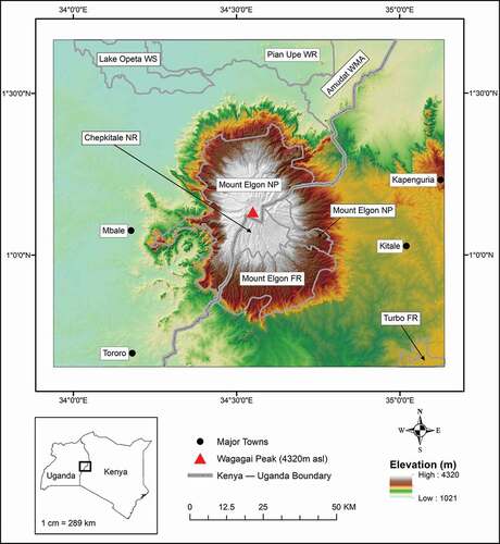
The current study was conducted in the MEE located in western Kenya and eastern Uganda (Figure 1). The area is approximately 15,000 km² and extends from 1°37ʹ42.82” N, 33°55ʹ45.07” E to 0°42ʹ15.76” N, 35°14ʹ18.84” E. The mountainous area rises from a plateau that lies about 1,850–2,000 meters above mean sea level (amsl) in the east and 1,050–1,350 meters amsl to the west (Hamilton & Perrott 1981). Its vegetation is zoned by altitude (Petursson, Vedeld, and Sassen 2013) and the montane Mount Elgon Forest (Doumenge et al. 1995) was gazetted in 1968 and 1992 in Kenya and Uganda respectively (Anseeuw and Alden 2010; Nakakaawa et al. 2015). The area is home to many important indigenous tree species (Petursson, Vedeld, and Sassen 2013) including giant groundsel (Senecio elgonensis) and Elgon olive (Olea hochstetteri) (Wasonga and Opiyo 2018). There are two rainy seasons in the MEE. Most of the rain falls between April and October on the Ugandan side (with annual averages of 1,500–2,000 millimeters) (Mugagga, Kakembo, and Buyinza 2012). The Kenyan side receives “long rains” between March and June – averaging 1,400–1,800 millimeters annually (Okello et al. 2010; Musau et al. 2015). The short rains, often received around October-December, have become more erratic and largely unpredictable over time. There is marginal temperature variation for the area (15°C-23°C) on the Ugandan side (Mugagga, Kakembo, and Buyinza 2012) and 14°C-24°C on the Kenyan side (Musau et al. 2015)). For mountainous regions like this, however, temperature and precipitation vary significantly with changes in altitude and relative location of windward and leeward sides of the mountain (see, for example, Van Den Hende et al. (2021)).

Figure 1. Map of the MEE in eastern Uganda and western Kenya. Elevation (meters amsl) and major protected areas are shown. Major towns are also shown for reference. It should be noted that FR is shorthand for forest reserve, NR is national reserve, NP is national park, WS is wetland system and WMA is wildlife management area

Significant interannual variability exists in the MEE landscape. This is attributed to various processes, including a substantial increase in post-2000’s precipitation, agricultural expansion (Wanyama, Moore, and Dahlin 2020) and complex LULC orientations (Petursson, Vedeld, and Sassen 2013). In addition, the MEE is composed of various microecosystems, thus some places have favourable climates (especially on higher altitudes) while others do not (at lower altitudes) (Mumba et al. 2016). This variability therefore impacts MEE livelihoods, which are also threatened by increasing natural hazards (e.g. floods, droughts, landslides) resulting from changing climate regimes.

2.2 Data sources

This study uses daily precipitation records from CHIRPS (Climate Hazards group Infrared Precipitation with Stations) (Funk et al. 2015), monthly maximum temperature records from CHIRTS (Climate Hazards Center Infrared Temperature with Stations) (Funk et al. 2019), 16-day NDVI from Moderate Resolution Imaging Spectroradiometer (MODIS) (Didan 2015), annual population density data from WorldPop (WorldPop Project 2020), and Shuttle Radar Topography Mission (SRTM) DEM from United States Geological Service (United States Geological Service 2000). CHIRPS data are available at 5 km spatial resolution and provide global daily and pentad records from 1981 to present. Daily records for the 1986–2018 period were obtained and preprocessed within Google Earth Engine (GEE) (Gorelick et al. 2017) and used to generate precipitation indices used in this study. CHIRTS data were created at the Climate Hazards Center (CHC) at University of California, Santa Barbara (Climate Hazards Center 2018), by blending gridded thermal infrared data with station data to create a seamless, high-resolution Tmax (maximum temperature) dataset that has been found to correlate very highly with observation data in the continent of Africa (Funk et al. 2019). This temperature dataset, for the 1986–2016 period, was used to compute temperature variables necessary for assessing the eco-environmental vulnerability of the MEE. NDVI data were obtained from MOD13Q1.V6, the 250 m, 16-day MODIS composite. This dataset, extending over the period 2001–2018, was obtained through AppEEARS, https://lpdaacsvc.cr.usgs.gov/appeears/ (AppEEARS Team 2019). The WorldPop population density dataset (WorldPop Project 2020) is available at 1 km spatial resolution (at the Equator) and 2000–2020 temporal coverage. This dataset, for the period 2001–2018, was used to assess changes in population density and distribution within the MEE. The SRTM DEM data, available at 30-m spatial resolution, were downloaded from GEE (Gorelick et al. 2017) and used to assess the effect of topography on general eco-environmental vulnerability of the MEE.

2.3 Generation and justification of variables used

The choice of criteria for evaluating vulnerability is crucial and one should identify criteria that are both representative and adaptable (Hou, Li, and Zhang 2015). Also, for easier interpretation, variables used in the EEVA should have a directly proportional relationship with eco-environmental vulnerability. Since the environment is highly dynamic and significantly impacted by both natural processes (e.g. precipitation distribution, drought occurrence, etc.) and human impacts (e.g. deforestation, afforestation, agricultural practices etc.), a reliable EEVA should consider both natural and social system variables. In this study, eco-environmental vulnerability of the MEE was assessed using both agriculture- and general environment-related variables. These variables were selected based on literature (Nguyen et al. 2016; Sahoo, Dhar, and Kar 2016; Simane, Zaitchik, and Foltz 2016; Parker et al. 2019), prior knowledge of the MEE, and insights from a 2019 field study in the area. Variables were selected to capture the effects of climate (precipitation and temperature), LULC change, population density and topography on the stability of an ecosystem that is heavily farmed, encroached and therefore experiencing significant interannual variability. All variables were normalized to range from 0 to 1 to allow for easier interpretation and comparison across variables. The variables were also resampled to 30-m spatial resolution.

While agriculture remains the mainstay for most of East Africa, its dependence on natural processes makes the sector highly vulnerable to the impacts of climate change and variability (Wanyama et al. 2019), thus influencing food insecurity in the region (Kotikot et al. 2018). The effect that variability in precipitation has on the stability of the region cannot be contested. Precipitation, combined with temperature, drives important ecosystem processes. Significant variability in precipitation will lead to ecological degradation which will disrupt nature-dependent systems and practices, like rain-fed agriculture. For instance, under RCP 4.5 and 8.5, the 2070s climate will drive significant changes in spatial distribution of maize cropping in Kenya (e.g. some currently suitable areas in Narok and Siaya counties will become unsuitable for currently grown maize cultivars, while currently unsuitable areas in Nakuru and Kericho will become suitable) (Kogo et al. 2019). This shift in suitability therefore means that maize will replace some higher-value cash crops (e.g. tea in Kericho), thus amplifying the economic effects of climate change. Even with some projected increases in precipitation, the agricultural sector is unlikely to benefit because of other unfavourable aspects (e.g. timing and spacing of rainfall) (Bryan et al. 2013). In response to diminishing yields, and exacerbated by substantially increasing populations, many people have expanded land under agriculture, often at the expense of natural vegetation (Maitima et al. 2009; Wanyama, Moore, and Dahlin 2020). Thus, variability in precipitation, coupled with significant warming trends, poses a substantial threat to the sustainability of both the environment and agricultural sector. In this study, eco-environmental vulnerability related to precipitation variability was assessed. Three precipitation variables were computed from daily records, including number of dry days (NDD), number of extreme events (NXE) and precipitation Z-scores during the growing season. Here, a dry day was defined as any day, between April 1 and June 30 (AMJ), when total precipitation amount was less than or equal to 2 mm. NDD was used to assess the influence of water shortage that occurs within the growing season, thus having negative influence on crop growth and yield. Therefore, the higher the NDD, the more vulnerable the area is. An extreme event was defined as any day within AMJ when precipitation exceeded 20 mm. NXE was used to evaluate the occurrence of extreme rainfall events within the growing seasons, events that likely induce flooding that destroys crops, property, and lives. The higher the NXE, the higher the vulnerability of the area. These two variables were defined following Haghtalab, Moore, and Ngongondo (2019), (2020)). Precipitation Z-scores were calculated by first computing total precipitation amounts for AMJ for each year from 1986 to 2018 and calculating a long-term mean (LTM) and standard deviation (LTSD). Then, the LTM was subtracted from each year’s total precipitation and the result divided by the LTSD (Equation 1(1) $\frac{Z_a=X_a-LTM}{LTSD}$(1) ). 1986–2018 was used because the same period was used in the preceding study in the MEE (Wanyama, Moore, and Dahlin 2020), but also because 34 years are enough for an accurate estimation of climatology (Winkler et al. 2018).

(1) $\frac{Z_a=X_a-LTM}{LTSD}$(1)

where $Z_a$ is the Z-score for year a; $X_a$ is the AMJ total precipitation amount for year a; LTM is the long-term mean; and LTSD is the long-term standard deviation.

Precipitation Z-score was specifically meant to detect drying patterns in MEE precipitation, so all values with positive Z-scores were set to 0. To establish a directly proportional relationship with eco-environmental vulnerability, values were transformed to absolute non-negative values. As such, highest values were indicative of highest eco-environmental vulnerability.

Persistent warming has been reported in East Africa since 1960s (Githui 2008; Ongoma and Chen 2017; Musau et al. 2018) with a warming of 1.5–2.0°C observed over the past 5 decades (Daron 2014). These high temperatures result in higher evapotranspiration rates (Seneviratne et al. 2012; Wanyama et al. 2019; Ayugi et al. 2020) and this has been linked to an observed or projected increase in frequency and intensity of droughts (Nguvava, Abiodun, and Otieno 2019; Ayugi et al. 2020). Since the majority of the MEE depends heavily on rain-fed agriculture, such warming and intensified droughts have adverse impacts on farming practices and ultimately on local livelihoods. For example, higher evaporation reduces the amount of water available to the crops (Wanyama et al. 2019) and higher temperatures accelerate crop growth leading to lower yields due to reduced gap-filling (Hatfield and Prueger 2015). Therefore, to characterize the influence of the warming on eco-environmental stability, temperature Z-scores were calculated in a similar fashion as precipitation Z-scores above. However, the temperature data spanned 1986–2016 (CHIRTS data are currently available until 2016) and temperature means over AMJ were calculated. Since this variable was meant to detect warming patterns in MEE temperatures, all negative Z-scores were set to 0. As such, the highest values indicate locations of highest vulnerability.

Vegetation coverage and population changes are both important factors influencing eco-environmental processes. LULC change (driven by, among other factors, increasing populations and a changing climate) has far-reaching impacts ranging from ecological, physical and socioeconomic effects (Pellikka et al. 2013) (for instance, see Salazar et al. (2015), Feddema et al. (2005), Turner II et al. (2007), and Mugagga et al. (2015)). These changes can alter land-atmosphere interactions, hence modifying local and global climates. In heavily agricultural areas with consistently increasing populations like the MEE, such changes present a significant threat to both the environment and people’s livelihoods. In this study, changes in vegetation greenness were assessed using NDVI anomalies (deviations from LTM). First, AMJ seasonal means were calculated for each year (2001–2016). Then, anomalies were generated for each year using the “anomalize” function in the “remote” package in R (Appelhans et al. 2016). Since this variable was used to assess the effect of generally decreasing greenness due to major activities (like deforestation) and subtle changes (like vegetation degradation), all positive anomalies were set to zero. Values were then transformed to absolute (non-negative) values to establish a directly proportional relationship with eco-environmental vulnerability. Therefore, locations with little or no tree cover will have to cope with higher eco-environmental vulnerability compared to highly vegetated areas like forests.

Assessing changes in population was necessary in this study because many studies have linked population growth to major LULC changes (Metzger et al. 2006; Wu and Zhang 2012; Ayuyo and Sweta 2014) that greatly influence eco-environmental stability. For instance, regions with quickly increasing populations have experienced significant expansion of land under agriculture and settlement as communities strive to increase food production. Also, sparsely populated areas like savannas and grasslands generally experience less anthropogenic interference and are therefore more stable compared to overpopulated areas. In this study, several population density variables were generated and assessed; ultimately, raw values were found suitable. The existence of extreme values (mainly in urban areas) affected distribution of values in less densely populated areas, and therefore, population distribution patterns were hardly detectable. For this reason, a cutoff value was explored. To find outliers for each year, we used the “boxplot.stats” function in “grDevices” package (R Core Team 2016). Here, we computed boxplot statistics (minimum, lower quartile, median, upper quartile, and maximum values) and returned values of data points less than (greater than) the minimum (maximum). From these, we selected the minimum value to create a series of “minimum extreme values” for 2001–2018, and the cutoff was calculated as the median value from this series. All pixel values greater than the cutoff were then set to this value (Equation 2(2) $\mathrm{I}\mathrm{F}\mathrm{P}\mathrm{O}{\mathrm{P}}_{\mathrm{n}}>\mathrm{C}\mathrm{U}\mathrm{T}\mathrm{O}\mathrm{F}\mathrm{F},\mathrm{t}\mathrm{h}\mathrm{e}\mathrm{n}\mathrm{P}\mathrm{O}{\mathrm{P}}_{\mathrm{n}}=\mathrm{C}\mathrm{U}\mathrm{T}\mathrm{O}\mathrm{F}\mathrm{F},\mathrm{e}\mathrm{l}\mathrm{s}\mathrm{e}\mathrm{P}\mathrm{A}\mathrm{S}\mathrm{S}$(2) ). This variable was used to assess the contribution of population density to eco-environmental vulnerability of the MEE.

(2) $\mathrm{I}\mathrm{F}\mathrm{P}\mathrm{O}{\mathrm{P}}_{\mathrm{n}}>\mathrm{C}\mathrm{U}\mathrm{T}\mathrm{O}\mathrm{F}\mathrm{F},\mathrm{t}\mathrm{h}\mathrm{e}\mathrm{n}\mathrm{P}\mathrm{O}{\mathrm{P}}_{\mathrm{n}}=\mathrm{C}\mathrm{U}\mathrm{T}\mathrm{O}\mathrm{F}\mathrm{F},\mathrm{e}\mathrm{l}\mathrm{s}\mathrm{e}\mathrm{P}\mathrm{A}\mathrm{S}\mathrm{S}$(2)

where $PO{P}_n$ is the population density for year n; $CUTOFF$ is the cutoff value; and PASS means “do nothing.”

Eco-environmental vulnerability is also strongly influenced by topographic variables (e.g. elevation, slope, and slope aspect). These variables play an important role in defining landscape conditions and determining the features of the land surface (e.g. potential for natural hazards, incoming solar radiation and LULC types (Eliasson et al. 2010; Nguyen and Liou 2019)). Elevation greatly influences regional climate regimes, evapotranspiration, and soils (Nguyen et al. 2016). Temperatures are known to decrease with increase in altitude (Mbiriri, Mukwada, and Manatsa 2018) and some locations receive more rainfall than others, depending on their orientation relative to the mountain. Slope, on the other hand, influences various physical processes. For instance, magnitude of slope and general “hilliness” of an area influence rainfall amounts received. Slope also influences soil erosion and landslides, with steeper slopes posing a higher risk for occurrence. Due in part to its topographic orientation, the MEE consists of various microecosystems, with higher altitudes generally exhibiting favourable climates compared to lower altitude areas (Mumba et al. 2016). Thus, two topographic variables (elevation and slope) were used to assess the effect of topography on eco-environmental vulnerability. For elevation, a cutoff value was first obtained at the 90^th percentile. Higher values were then set to this cutoff (like population density above) since these generally represented stable mountain locations unpopulated by humans. Percent slope was also calculated, and values higher than 30 percent were excluded, because slopes higher than this generally limit access and diminish land suitability for some socio-economic activities (e.g. maize farming) (Wang 2015; Wanyama et al. 2019).

2.4 Methods

This section describes the methods and analyses performed to characterize patterns of eco-environmental vulnerability in the MEE. The analyses included computing EEVI, assessing spatio-temporal patterns of change in multi-year variables, and characterizing precipitation concentration in the MEE. These analyses were performed in R (R Core Team 2018).

2.4.1 Spatial principal components analysis

To compute an EEVI for the MEE, this study implemented principal components analysis (PCA), which has been applied in various studies (Li et al. 2006; Hou, Li, and Zhang 2015; Zou and Yoshino 2017). PCA reduces the dimensionality of data, increasing interpretability while minimizing loss of information (Pearson 1901). It linearly transforms original variables into a set of uncorrelated variables (called principal components, PCs), thus making it one of the simplest dimensionality reduction techniques (Jolliffe 1990). PCA can be expressed as follows:

(3) $Y=\hspace{0.17em}{n}_1{x}_1+\hspace{0.17em}{n}_2{x}_2+\hspace{0.17em}{n}_3{x}_3+\hspace{0.17em}{n}_{\mathrm{m}}{x}_{\mathrm{m}}$(3)

where Y is the PC score; n is the component loading; x is the measured value of a variable; and m is the total number of variables (Hou, Li, and Zhang 2015).

The importance of a PC is ranked, denoted by eigenvalues, based on the amount of variance it captures in the original data (Hou, Li, and Zhang 2015; Zou and Yoshino 2017). For spatial data, SPCA is used and the technique transforms attributes in a multiband spatial dataset into a new multivariate space whose axes are rotated with respect to the original space (Hou, Li, and Zhang 2015; Zou and Yoshino 2017).

SPCA was used in this study to decompose climate, topography, population density and vegetation greenness variables to generate annual EEVI for the MEE (for 2001–2016). SPCA was a suitable method since there was no clear understanding of the nature of patterns within these variables (Hou, Li, and Zhang 2015). The “rasterPCA” function in the “RStoolbox” package (Leutner et al. 2019) in R statistical software was used. SPCA results were assessed and for each year, the first five PCs were retained to compute EEVI using the equation below.

(4) $EEV{I}_i=\hspace{0.17em}{n}_{1}P{C}_1+\hspace{0.17em}{n}_{2}P{C}_2+\hspace{0.17em}{n}_{3}P{C}_3+\hspace{0.17em}{n}_{4}P{C}_4+n_{5}P{C}_5$(4)

where $EEV{I}_i$ is the eco-environmental vulnerability index for year i; $P{C}_1$ is the first principal component; and $n_1$ is the contribution ratio of the first principal component (Hou, Li, and Zhang 2015).

The computed EEVI surfaces were reclassified into five qualitative groups indicative of different levels of eco-environmental vulnerability in the MEE. The equal interval classification scheme was applied, although other data classification schemes were explored. The scheme is useful when the objective is to put emphasis on the amount of an attribute value relative to another value (Torresan et al. 2012). Therefore, this method allowed for comparison of EEVI across years. This classification scheme has previously been used in similar studies (Torresan et al. 2012; Žurovec, Čadro, and Sitaula 2017; Parker et al. 2019). Table 2 shows class ranges used in this study.

Table 1. Properties of datasets used in this study

Dataset	Spatial Resolution	Temporal Resolution	Source
Precipitation	5 km	1986–2018	CHIRPSDaily (Funk et al. 2015)
Temperature	5 km	1986–2016	CHIRTSMax Monthly (Funk et al. 2019)
SRTM DEM	30 m	2000	United States Geological Service (United States Geological Service 2000)
NDVI	250 m	2001–2018	MODIS (Didan 2015)
Population density	1 km	2001–2018	WorldPop (WorldPop Project 2020)

Table 2. Value ranges for different levels of eco-environmental vulnerability in the MEE

Class	Range
Potential	0.383–0.586
Slight	0.181–0.383
Light	−0.022–0.181
Moderate	−0.225 – −0.022
Severe	−0.427 – −0.225

PCA was also performed on each of the original temporal series of NDVI, temperature, precipitation, and population density variables. This temporal PCA (TPCA) was necessary to identify persistent patterns of change in each variable over time. To do this, time series rasters of these variables (2001–2018 for precipitation, NDVI and population density, and 2001–2016 for temperature) were used, and only PCs explaining more than 1% of the variance were considered significant.

2.4.2 Precipitation concentration index

Given that significant changes in precipitation have been reported previously, especially post-2000 (Wanyama, Moore, and Dahlin 2020), this study assessed spatio-temporal changes in distribution of MEE precipitation over 34 years (1986–2018). Monthly precipitation totals for this period were used to compute the PCI (Oliver 1980; De Luis et al. 2011). PCI was preferred in this study because it is a powerful measure of precipitation distribution over time (De Luis et al. 2011). The index was calculated on two scales: annual and supra-seasonal. The supra-seasonal ranges were defined generally as wet (January–June) and dry (July–December). The annual and supra-seasonal PCI were computed according to Equations 5(5) $\mathrm{P}\mathrm{C}{\mathrm{I}}_{annual}=\frac{{\sum }_{i=1}^{12}{p}_i^2}{{\left({\sum }_{i=1}^{12}{p}_i\right)}^2}\ast 100$(5) and 6(6) $\mathrm{P}\mathrm{C}{\mathrm{I}}_{supraseasonal}=\frac{{\sum }_{i=1}^6{p}_i^2}{{\left({\sum }_{i=1}^6{p}_i\right)}^2}\ast 50$(6) , respectively.

(5) $\mathrm{P}\mathrm{C}{\mathrm{I}}_{annual}=\frac{{\sum }_{i=1}^{12}{p}_i^2}{{\left({\sum }_{i=1}^{12}{p}_i\right)}^2}\ast 100$(5)

(6) $\mathrm{P}\mathrm{C}{\mathrm{I}}_{supraseasonal}=\frac{{\sum }_{i=1}^6{p}_i^2}{{\left({\sum }_{i=1}^6{p}_i\right)}^2}\ast 50$(6)

where $p_i$ is the monthly precipitation in month i (De Luis et al. 2011).

PCI values range from 8.3 (uniform precipitation concentration) to 100 (irregular precipitation distribution) with increasing values denoting an increased monthly precipitation concentration (Oliver 1980). Oliver (1980) proposed that, on the annual and supra-seasonal scales, PCI values less than 10 indicate uniform precipitation distribution (lowest precipitation concentration), values between 11 and 20 show a seasonal distribution while values greater than 20 denote an irregular distribution. In this study, the PCI was used to prove that distribution of MEE precipitation has significantly changed over time. As such, the Mann-Whitney U test, a non-parametric test, was applied to assess the statistical difference in precipitation concentration between the first 11 years (1986–1996) and last 11 years (2008–2018). The 11-year periods were used here because they were used in a previous study for the same study area (Wanyama, Moore, and Dahlin 2020). Such statistical comparison has been performed in previous studies (De Luis et al. 2011; Kibret et al. 2019). PCI change results were assessed at the 95% significance level.

3 Results

This study characterizes, using SPCA, TPCA and PCI, patterns of eco-environmental vulnerability in the MEE. The results highlight levels of eco-environmental vulnerability and areas of persistent changes in precipitation, NDVI, and population density. Results from PCI analysis are also presented and, together, attempt to comprehensively characterize eco-environmental vulnerability and the variability observed over the MEE.

3.1 Eco-environmental vulnerability

3.1.1 SPCA results

The first five PCs were retained to compute EEVI in this study. Together, these PCs explained more than 95% of the variance in the original eight variables included in the study. An example of the breakdown of variable loadings is shown in Tables 3, 4 and 5 for 2001, 2008 and 2016, respectively. Figures 2 and 3 show the five PCs in 2001 and 2016. The amount of variance captured by each PC varied over time, and generally, the first PC averagely accounted for about 50%. This PC was heavily loaded on elevation, slope and NXE variables.

Table 3. Loadings for the first five PCs in 2001. Note that major loadings for each PC are shown in bold.

Variable	PC1	PC2	PC3	PC4	PC5
Elevation	0.842	0.051	0.430	0.316	0.005
Slope	0.457	−0.185	−0.860	−0.014	−0.128
Precipitation Z-scores	0.018	0.002	0.004	0.057	0.000
Temperature Z-scores	0.000	0.000	0.000	0.000	0.000
Number of dry days	0.155	0.174	0.157	−0.661	−0.676
Number of extreme events	0.232	−0.137	0.063	−0.677	0.676
NDVI	−0.045	−0.072	−0.030	0.037	0.163
Population density	−0.046	−0.953	0.212	−0.006	−0.207

Table 4. Loadings for the first five PCs in 2008. Note that major loadings for each PC are shown in bold.

Variable	PC1	PC2	PC3	PC4	PC5
Elevation	0.841	0.013	0.322	0.280	0.241
Slope	0.449	−0.101	−0.777	−0.425	−0.007
Precipitation Z-scores	0.084	−0.099	0.423	−0.703	0.252
Temperature Z-scores	−0.103	0.091	−0.039	−0.177	−0.159
Number of dry days	0.110	0.139	0.324	−0.426	−0.517
Number of extreme events	0.241	−0.060	0.029	0.183	−0.763
NDVI	0.003	0.019	−0.002	−0.005	0.001
Population density	−0.052	−0.974	0.083	0.031	−0.063

Table 5. Loadings for the first five PCs in 2016. Note that major loadings for each PC are shown in bold.

Variable	PC1	PC2	PC3	PC4	PC5
Elevation	0.849	0.055	0.451	0.251	0.064
Slope	0.461	0.107	−0.878	0.010	−0.072
Precipitation Z-scores	0.000	0.000	0.000	0.000	0.000
Temperature Z-scores	−0.000	0.002	0.002	−0.004	0.009
Number of dry days	0.012	−0.055	0.082	0.006	−0.973
Number of extreme events	0.223	0.057	0.113	−0.966	0.000
NDVI	0.072	0.005	0.045	0.038	−0.204
Population density	−0.110	0.989	0.068	0.041	−0.049

Figure 2. The first five PCs used to compute EEVI for 2001

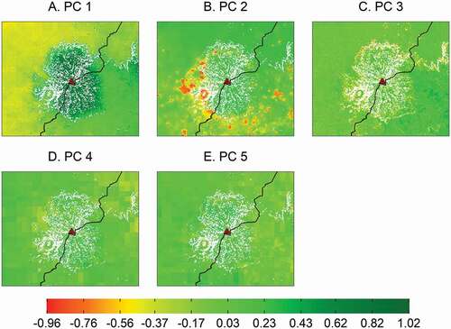
Figure 3. The first five PCs used to compute EEVI for 2016. It should be noted that the scale in this figure is same as in Figure 2

The second PC, which explained about 25% of the variance, was loaded mostly on population density. Notice that the loading for this PC shifts between positive and negative (Tables 3, 4 and 5), thus introducing the visible changes in distribution of the PC values over the years (e.g. compare Figures 2b and 3b). The third PC (approx. 10% of variance) was mostly a linear function of slope and elevation, as well as climate variables in some years (see Table 4). Loadings of the fourth and fifth PCs exhibited major changes from year to year, but climate variables (NXE and NDD) together with elevation were common components. These two PCs explained about 10% of the variance in the original data.

3.1.2 Eco-environmental vulnerability index

In this study, eco-environmental vulnerability was defined as the risk of damage to the natural environment (Nandy et al. 2015). As such, this study was conducted to evaluate the natural resource system affected by both natural and human activities within the MEE. Results show that 38% of the MEE (5,700 km²) is moderately vulnerable (Figure 4). These areas are mostly grasslands and agricultural land in the northwestern and western parts of the MEE, respectively. Highest proportions of this vulnerability level were observed in 2005 (52%), 2008 (50%), 2001 (47%), 2012 (45%) and 2014 (43%) when most of the savannas were also moderately vulnerable. The second highest proportion of the MEE was lightly vulnerable, and these areas majorly included areas in the southeastern MEE, which are primarily composed of mixed land uses (cropland, shrubland, grassland). This vulnerability class was the most static of all, as no major changes in proportion and locations were observed across the 16-year period (with percent proportions ranging from 24 to 29%).

Figure 4. EEVI for each year from 2001 to 2016. Notice that eco-environmental vulnerability varies over time, but persistent patterns exist in space. EEVI increases with decrease in elevation

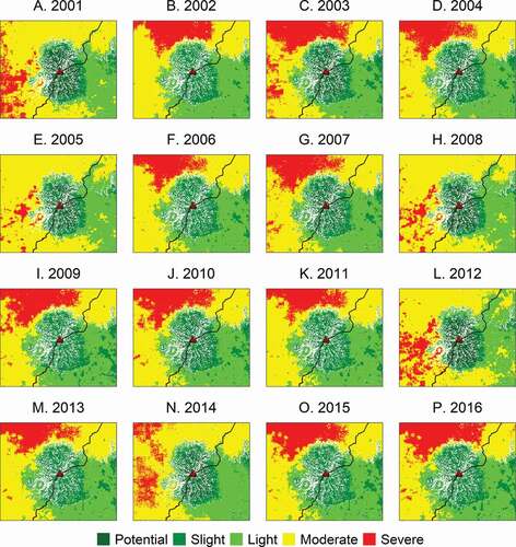
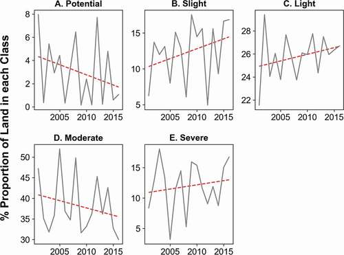
There was generally an equal proportion of land in the severe and potential vulnerability classes (both averaging 12% (1,800 km²) over the 16 years). High elevation (>2,000 m amsl) locations on the Afromontane forest constituted the slight vulnerability class, and these generally remained stationary throughout the study period. On the other hand, savannas in northern MEE represented most of the land under the severe class, although some agricultural lands in eastern MEE were also found in this class, especially during 2001, 2003, 2008, 2012 and 2014. Some of the high elevation areas of Mount Elgon fell into the smallest class (proportions ranging from <1 percent to about 8%). Land under this class was highest in 2001, 2012 and 2008 (1,200 km², 1,200 km²and 1,000 km², respectively) and least in 2009, 2011 and 2013 (approx. 20 km², 30 km² and 30 km², respectively). It is worth mentioning that the proportion of land under the potential and moderate vulnerability classes exhibited a generally decreasing trend over time (Figure 5a and d), while a positive trend was observed in the slight, light, and severe vulnerability classes (Figure 5b,c and e).

Figure 5. Percent proportion of land under each EEVI class from 2001 to 2016. The red lines represent fitted linear trends for each series

3.1.3 TPCA results

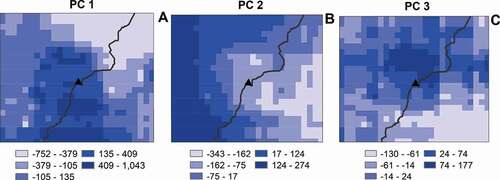
Results from decomposing the temperature time series (2001–2016) are not provided because no significant patterns in MEE temperatures were found. For precipitation time series (2001–2018), each of the first three PCs explained more than 1% of the variance. PC1 revealed the general spatial distribution of precipitation in the MEE (Figure 6a). Savanna and grasslands in northeastern MEE are the driest while the Afromontane forest and parts of southern MEE are the wettest. The second and third PCs (Figures 6b and C) showed varying trends in precipitation possibly related to topography. Such persistent changes in precipitation may be responsible for major changes in eco-environmental vulnerability over the years (Figure 4).

Figure 6. Important PCs obtained from the precipitation time series (2001–2018) using TPCA

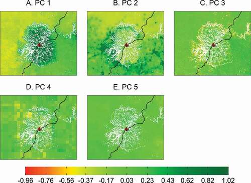
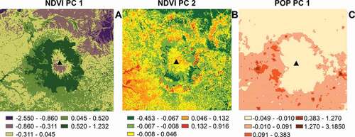
The first two PCs from the NDVI time series (2001–2018) decomposition contained important information. PC1 captured the distribution of major LULCs in the MEE (Figure 7a). Here, the Afromontane forest in central MEE, savanna and grasslands in north and northeast, and agricultural land were all identified. Equally interesting is PC2 (Figure 7b) which delineated locations of major greening (in the northern MEE and high elevation areas of the mountain) and browning (especially in southwestern MEE and the edges of the mountain forest). Results from decomposing the population density time series (2001–2018) revealed the general distribution of the population in the MEE (Figure 7c). Here, urban centers and other highly populated areas (mostly agricultural lands) were identified. Least populated areas were found in most of the savannas and grasslands as well as high elevations.

Figure 7. The first two PCs from NDVI time series (a and b) and the first from population density time series (c)

3.2 Precipitation concentration in the MEE

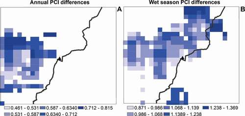
Assessment of PCI over the dry period yielded only a few locations in southwestern MEE with significantly different precipitation concentration between 1986–1996 (first 11 years) and 2008–2018 (last 11 years). This result is not provided in this study. Figure 8 shows locations where PCI values for 2008–2018 were greater than 1986–1996 for both the annual (Figure 8a) and wet season (Figure 8b) periods. In these locations, there is a more than likely probability (p < 0.05) that precipitation concentration was greater in the later period than the previous. This is especially true for western MEE (on the annual scale) and the west-to-northeastern stretch of the MEE (for the wet season).

Figure 8. Locations where precipitation concentration in last 11 years (2008–2018) was significantly (p < 0.05) greater than the first 11 years (1986–1996)

4 Discussion

4.1 Eco-environmental vulnerability in the MEE

Climate change continues to affect most developing nations, especially those relying on rainfed agriculture (Wanyama, Moore, and Dahlin 2020). The vulnerability of the agriculture sector is worsened by the intensifying and more frequent natural disasters coupled with significant environmental change. In the MEE, a largely agricultural area, populations have increased to approximately 1,000 people per km² in some areas (Nakakaawa et al. 2015; Vlaeminck et al. 2016). Here, farm sizes are consistently shrinking as populations increase, and this signals mounting pressure on land (Nakakaawa et al. 2015; McKinney and Wright 2021). The need to increase food production has fueled encroachment on ecologically fragile land (Nakileza and Nedala 2020) and illegal access to PAs (McKinney and Wright 2021). As a result, this LULC change has, in part, modified local ecosystem functioning (Omwenga, Daudi, and Jebet 2019), intensified climate-related hazards (Nakakaawa et al. 2015; EAC et al. 2016) and introduced and/or increased significant interannual variability (Wanyama, Moore, and Dahlin 2020). Moreover, precipitation concentration is amplifying notably in the wet season (Figure 8), thus adding another layer of risk for agriculture and ultimately for local community livelihoods. These complex human-environment interactions in the MEE therefore underpin the region’s eco-environmental vulnerability. Yet characterizing this vulnerability is marred by the absence of data at appropriate spatial and temporal scales and inadequacies in practical methodologies.

Representing vulnerability as a single index provides important information about the degree of vulnerability, and helps identify most vulnerable regions (Žurovec, Čadro, and Sitaula 2017) where action can be targeted. Outputs from these analyses are maps that generally reflect the kind of datasets and methods used, as well as decisions about data aggregation, variable weighting and resolution of the analysis (Abson et al. 2012). PCA has commonly been used in these studies, especially when no prior knowledge exists about patterns in the variables (Hou, Li, and Zhang 2015). PCA does not weight original variables; rather, it provides relative vulnerability relating to how individual drivers of vulnerability co-vary in space (Abson et al. 2012; Defne et al. 2020). It is therefore a good source of information about how multiple variables interact, aggregate and affect a given location (Defne et al. 2020). This is important, as human-environment systems are known to have complex interactions and therefore intricate interrelationships among biophysical and socio-political factors. By aggregating these variables into a single vulnerability index, therefore, locations experiencing highest cumulative vulnerability can be delineated. This does not mean that important underlying information about the variables is lost; policymakers can assess the retained PCs and identify, based on their knowledge, drivers or types of vulnerability that are most important in their context (Abson et al. 2012).

The present study found that majority of the MEE (comprising savannas, grasslands, and most of the agricultural land in Ugandan MEE) was moderately vulnerable based on the analysis methods and variables used. A majority of the savannas and grasslands were severely vulnerable, and this has also been reported elsewhere by Jiang et al. (2018). Eco-environmental vulnerability also varies in time with increases in the “slight,” “light” and “severe” categories. This temporal dependence means that eco-environmental vulnerability is a function of multiple local factors, often operating at a range of space and time scales. This dynamic nature constrains the validity of vulnerability scores to specific scales (Aretano et al. 2015). The temporal variability in eco-environmental vulnerability over the 2001–2016 period was related to multi-year variables derived from precipitation (NDD, NXE, precipitation Z-scores), temperature (temperature Z-scores) and population density. Therefore, it can be inferred that the MEE will continue to experience significant interannual variability in eco-environmental vulnerability as the climate system changes and populations increase particularly in the northwestern part of the domain (Figure 4). It should also be noted that, being mountainous, topographic variables (elevation and slope) also had a substantial influence on the vulnerability of the MEE – with EEVI markedly increasing with decrease in elevation. Previous studies have also found that topographic characteristics and precipitation significantly influence eco-environmental vulnerability (Nguyen et al. 2016; Jiang et al. 2018; Li, Shi, and Wu 2021).

Atzberger (2013) stated that, under climate change, society is tasked with increasing food production while fostering sustainability of Earth’s environmental systems. Results from this study are aimed at steering action towards achieving this goal in the MEE, by providing policymakers and development practitioners with valuable and comprehensive knowledge of the varying levels of eco-environmental vulnerability in the MEE and identifying areas that require immediate conservational attention. As seen over the years, savannas and grasslands are mostly severely or moderately vulnerable. This is not shocking, as these areas (i) are increasingly being inhabited by humans who introduce major LULC changes (e.g. natural vegetation to agriculture) (Wanyama, Moore, and Dahlin 2020), (ii) receive the least amounts of rainfall (Figure 6A), and (iii) are uncharacteristically warming over time. The erratic rainfall in these areas means that rainfed agriculture is not a reliable source of livelihood and the increasing temperatures make pastoralism a risky venture. Most agricultural areas in the west and southwestern MEE exhibit moderate eco-environmental vulnerability. This may be driven by a significantly changing and/or varying climate, although the intensifying human activities in these areas are also to blame. For instance, the expansion of land under agriculture at the expense of natural vegetation has a long-term effect of modifying ecosystem processes and accelerating climate change and variability. These areas include some of the most populated areas in rural Africa – meaning that majority of the MEE population is substantially vulnerable to climate change and related environmental change, and that this vulnerability is likely to rise with rising populations.

Despite its socio-ecological importance and the complex human-environment interactions influencing its stability, the MEE has been understudied. This is due in part to the acute data inadequacies in this area and the rest of East Africa. In some cases, data (e.g. from national census) are available but only at mismatched spatial and temporal scales and/or in aspatial formats that limit their usage. Through recent developments in Earth observation technologies and modeling techniques, valuable spatio-temporally contiguous data have been produced and are now being accessed freely and used to conduct important environmental assessments including EEVA. This study leverages globally available multi-decadal data (MODIS NDVI, CHIRPS, CHIRTS, and WorldPop) and open-source software (R and GEE) to assess eco-environmental vulnerability. This is a demonstration that this analysis can easily be translated to regions with similar characteristics (e.g. other mixed forest and agriculture landscapes like the Mau Complex in Kenya, Mount Kilimanjaro in Tanzania, among others). Additionally, using these datasets enables important ecosystem properties like EEVI to be characterized and monitored over time, thus ensuring better planning and decision making for environmental conservation and local livelihood improvement.

This study found that areas surrounding PAs are at great risk of deforestation and forest degradation (e.g. see Figure 7b), corroborating results by Wanyama, Moore, and Dahlin (2020). MEE PAs have also been influenced by activities such as overexploitation of forest resources by logging companies and post-independence political changes, mainly due to institutional deficiencies (Petursson and Vedeld 2017). This result shows that there is a spatial structure to eco-environmental vulnerability, and this is key as it can inform policymakers about factors driving ecosystem vulnerability in the MEE. The amplifying precipitation concentration (Figure 8) also means that the MEE climate is significantly changing and consequently diminishing MEE’s ability to support rainfed agriculture, a major source of livelihood for majority of the local population. Conservation of this ecosystem is therefore imperative, and this study recommends that areas in the moderate and severe vulnerability classes should especially be targeted. To achieve this, policies aimed at protecting PAs and other natural lands should be better enforced. One such way is the adoption of the bottom-up approach in which local community members’ opinions are considered in conservation and resource management decision-making. As Tadesse, Woldetsadik, and Senbeta (2017) note, this approach is key to mobilizing local community participation in conservation of common-pool natural resources. The approach provides a great avenue to (i) gather important indigenous knowledge systems from the people, (ii) boost ownership and garner the support of communities, and (iii) ultimately ensure successful implementation of projects and policies. Gashu and Aminu (2019) concluded that natural resource management is impossible without proper involvement of local communities. The study also found that EEVI is significantly driven by human activities either directly (e.g. increasing populations, clearing forests for agriculture) or indirectly (e.g. changing precipitation patterns due to deforestation). Therefore, acknowledging that people are major players in this ecosystem is an important step toward simultaneously conserving the environment and improving livelihoods. Against this background, this study recommends that positive behavior change should be encouraged and funded among local communities. This includes adopting lifestyles and habits that foster more sustainable use of natural resources. Efforts aimed at curbing the widespread conversion of natural vegetation to croplands and settlement are especially encouraged. On the same account, the role of natural vegetation in regulating the local climate system should be emphasized.

4.2 Sources of uncertainty

There is no rule of thumb as to how many variables should be used in EEVA (Nguyen et al. 2016), and each study defines its variables based on contexts and available data. Data unavailability is a widely known problem in East Africa. Due to this shortcoming, data used in this study were available at multiple and mostly very coarse spatial resolutions: the DEM was obtained at 30 m, population density at 1 km and CHIRPS and CHIRTS at 4 km. This scale mismatch introduced some uncertainties in the EEVA results. Additionally, the present study would have benefited from census data for Kenya and Uganda. From these, more specific demographic variables associated with eco-environmental vulnerability would have been computed and incorporated in the study to produce a more detailed picture of eco-environmental vulnerability. However, the census is conducted once every 10 years in these countries and therefore would mismatch the temporal scale of analysis (annual) used in this study. It is also worth noting that even this decadal data was not available. In its place, population density data from WorldPop, which have been used in previous studies in Africa (Kibret et al. 2019; McNally et al. 2019; Helman and Zaitchik 2020), were used. Further, the study design and interpretation of the results were based in part on prior knowledge of the MEE, and insights from a 2019 field study in the area.

5 Conclusions

The present study found that the majority of the MEE (comprising savannas, grasslands, and most of the agricultural land in Ugandan MEE) was moderately vulnerable based on the analysis methods and variables used. EEVI showed a marked increase in vulnerability with decrease in elevation. EEVI is most severe in the savannas of the northwestern part of the domain. Savannas and grasslands constituted the majority of the severe vulnerability class. Eco-environmental vulnerability varied from year to year, indicating that it is a function of multiple factors operating at numerous scales (local to coarse scale). Eco-environmental vulnerability in the MEE is strongly associated with multi-year variables based on precipitation, temperature, and population density. With fast increasing populations and intensifying climate change and variability, eco-environmental vulnerability in the MEE will continue to experience significant interannual variability. Moreover, precipitation concentration is amplifying especially in the wet season, thus adding another layer of risk for agriculture and ultimately for local community livelihoods.

To achieve sustainability in the MEE ecosystem and the livelihoods it supports, areas in the moderate and severe vulnerability classes need prioritized conservation. It is recommended that environmental conservation policies be implemented and enforced in these areas by adopting the bottom-up approach in which local community members’ opinions are incorporated in decision making. In addition, more data must be collected and used. Communities can be encouraged to adopt lifestyles and habits that foster more sustainable use of natural resources, and international donors can use this information to target conservation activities.

Authors’ contributions

Dan Wanyama, Bandana Kar, and Nathan J. Moore designed the study; Nathan J. Moore and Bandana Kar supervised its implementation and contributed to the manuscript; Dan Wanyama performed the analysis and developed the manuscript.

Acknowledgements

Authors would like to thank the three anonymous reviewers for their comments which have greatly improved this manuscript. This study received support from multiple sources and authors would like to express their gratitude specially to Remote Sensing and GIS Research and Outreach Services (RS&GIS) at Michigan State University for funding the PhD studies within which this study was conducted. Additionally, authors thank Eliud Akanga for his valuable support in the 2019 field study whose insights were invaluable in this study. This manuscript has been authored in part by UT-Battelle, LLC, under contract DE-AC05-00OR22725 with the US Department of Energy (DOE).

Data availability statement

The study relied on publicly available datasets. Sources of these datasets are provided in Table 1.

Disclosure statement

No potential conflict of interest was reported by the author(s).

Additional information

Funding

This research was supported by funds from the College of Social Science at Michigan State University Graduate Office Fellowship (GOF) awarded in 2019 by College of Social Science and Department of Geography, Environment and Spatial Sciences at Michigan State University.

References

- Abson, D. J., A. J. Dougill, and L. C. Stringer. 2012. “Using Principal Component Analysis for information-rich socio-ecological vulnerability mapping in Southern Africa.” Appl Geogr [Internet] 35 (1–2): 515–524. doi:https://doi.org/10.1016/j.apgeog.2012.08.004.
- Aleksandrova, M., A. K. Gain, and C. Giupponi. 2016. “Assessing agricultural systems vulnerability to climate change to inform adaptation planning: an application in Khorezm, Uzbekistan.” Mitig Adapt Strateg Glob Chang [Internet] 21 (8): 1263–1287. doi:https://doi.org/10.1007/s11027-015-9655-y.
- Anseeuw, W., and C. Alden, editors. 2010. The struggle over land in Africa: Conflicts, politics and change. Cape Town, South Africa: HSRC Press.
- AppEEARS Team. 2019. Application for Extracting and Exploring Analysis Ready Samples (AppEEARS). Sioux Falls, SD, USA: LP DAAC.
- Appelhans, A. T., F. Detsch, T. Nauss, and M. T. Appelhans. 2016. “Remote: Empirical Orthogonal Teleconnections in R.“ Journal of Statistical Software 65 (10), 1–19. doi:https://doi.org/10.18637/jss.v065.i10
- Aretano, R., T. Semeraro, I. Petrosillo, A. De Marco, M. R. Pasimeni, and G. Zurlini. 2015. “Mapping ecological vulnerability to fire for effective conservation management of natural protected areas.” Ecol Modell [Internet] 295: 163–175. doi:https://doi.org/10.1016/j.ecolmodel.2014.09.017.
- Atzberger, C. 2013. “Advances in remote sensing of agriculture: Context description, existing operational monitoring systems and major information needs.” Remote Sens 5 (2): 949–981. doi:https://doi.org/10.3390/rs5020949.
- Aydi, A. 2018. “Evaluation of groundwater vulnerability to pollution using a GIS-based multi-criteria decision analysis.” Groundw Sustain Dev [Internet] 7: 204–211. doi:https://doi.org/10.1016/j.gsd.2018.06.003.
- Ayugi, B., G. Tan, N. Rouyun, D. Zeyao, M. Ojara, L. Mumo, H. Babaousmail, and V. Ongoma. 2020. “Evaluation of meteorological drought and flood scenarios over Kenya, East Africa.” Atmosphere (Basel) 11: 3.
- Ayuyo, I. O., and L. Sweta. 2014. “Land Cover and Land Use Mapping and Change Detection of Mau Complex in Kenya Using Geospatial Technology.” Int J Sci Res 3 (3): 767–778.
- Baca, M., P. Läderach, J. Haggar, G. Schroth, O. Ovalle, and B. Bond-Lamberty. 2014. “An integrated framework for assessing vulnerability to climate change and developing adaptation strategies for coffee growing families in mesoamerica.” PLoS One 9 (2): 2. doi:https://doi.org/10.1371/journal.pone.0088463.
- Boori, M. S., K. Choudhary, R. Paringer, and A. Kupriyanov. 2021. “Eco-environmental quality assessment based on pressure-state-response framework by remote sensing and GIS.” Remote Sens Appl Soc Environ [Internet] 23. doi:https://doi.org/10.1016/j.rsase.2021.100530.
- Brink, A. B., C. Bodart, L. Brodsky, P. Defourney, C. Ernst, F. Donney, A. Lupi, and K. Tuckova. 2014. “Anthropogenic pressure in East Africa - Monitoring 20 years of land cover changes by means of medium resolution satellite data.” Int J Appl Earth Obs Geoinf [Internet] 28 (1): 60–69. doi:https://doi.org/10.1016/j.jag.2013.11.006.
- Broeckx, J., M. Maertens, M. Isabirye, M. Vanmaercke, B. Namazzi, J. Deckers, J. Tamale, et al. 2019. “Landslide susceptibility and mobilization rates in the Mount Elgon region, Uganda.” Landslides 16 (3): 571–584. DOI:https://doi.org/10.1007/s10346-018-1085-y.
- Bryan, E., C. Ringler, B. Okoba, C. Roncoli, S. Silvestri, and M. Herrero. 2013. “Adapting agriculture to climate change in Kenya: Household strategies and determinants.” J Environ Manag. 114: 26–35. doi:https://doi.org/10.1016/j.jenvman.2012.10.036.
- Climate Hazards Center. 2018. CHIRTSmonthly [Internet]. [accessed 2020 July 3]. https://www.chc.ucsb.edu/data/chirtsmonthly
- Daron, J. D. 2014. Regional Climate Messages for East Africa. Ottawa, ON: CARIAA.
- De Luis, M., J. C. González-Hidalgo, M. Brunetti, and L. A. Longares. 2011. “Precipitation concentration changes in Spain 1946-2005.” Nat Hazards Earth Syst Sci 11 (5): 1259–1265. doi:https://doi.org/10.5194/nhess-11-1259-2011.
- Defne, Z., A. L. Aretxabaleta, N. K. Ganju, T. S. Kalra, D. K. Jones, and K. E. L. Smith. 2020. “A geospatially resolved wetland vulnerability index: Synthesis of physical drivers.” PLoS One [Internet] 15 (1): 1–27. doi:https://doi.org/10.1371/journal.pone.0228504.
- Didan, K. 2015. MOD13Q1 MODIS/Terra Vegetation Indices 16-Day L3 Global 250m SIN Grid V006. Sioux Falls, SD, USA: NASA EOSDIS Land Processes DAAC.
- Doumenge, C., D. Gilmour, M. R. Pérez, and J. Blockhus. 1995.“Tropical montane cloud forests: Conservation status and management issues.” Hamilton, L.S., Juvik, J.O., and Scatena, F.N. In Tropical montane cloud forests, 24–37. New York, NY: Springer.
- Duarte, L., A. C. Teodoro, J. A. Gonçalves, A. J. Guerner Dias, and J. Espinha Marques. 2015. “A dynamic map application for the assessment of groundwater vulnerability to pollution.” Environ Earth Sci 74 (3): 2315–2327. doi:https://doi.org/10.1007/s12665-015-4222-0.
- EAC, UNEP, GRID-Arendal. 2016. Sustainable mountain development in East Africa in a changing climate. Arusha, Tanzania: EAC.
- Eliasson, Å, R. J. A. Jones, F. Nachtergaele, D. G. Rossiter, J. M. Terres, J. Van Orshoven, H. van Velthuizen, K. Böttcher, P. Haastrup, and C. Le Bas. 2010. “Common criteria for the redefinition of Intermediate Less Favoured Areas in the European Union.” Environmental Science & Policy 13 (8): 766–777. doi:https://doi.org/10.1016/j.envsci.2010.08.003.
- Enea, M., and G. Salemi. 2001. “Fuzzy approach to the environmental impact evaluation.” Ecological Modelling 136 (2–3): 131–147. doi:https://doi.org/10.1016/S0304-3800(00)00380-X.
- FAO. 2016. The state of food and agriculture: climate change, agriculture and food security. Rome: FAO.
- Feddema, J. J., K. W. Oleson, G. B. Bonan, L. O. Mearns, L. E. Buja, G. A. Meehl, and W. M. Washington. 2005. “The Importance of Land-Cover Change in Simulating Future Climates.” Science 310 (80): 1674–1678. doi:https://doi.org/10.1126/science.1118160.
- Fetene, A., T. Hilker, K. Yeshitela, R. Prasse, W. Cohen, and Z. Yang. 2016. “Detecting Trends in Landuse and Landcover Change of Nech Sar National Park, Ethiopia.” Environ Manage 57 (1): 137–147. doi:https://doi.org/10.1007/s00267-015-0603-0.
- Funk, C., P. Peterson, M. Landsfeld, D. Pedreros, J. Verdin, S. Shukla, G. Husak, et al. 2015. “The climate hazards infrared precipitation with stations - A new environmental record for monitoring extremes.” Sci Dat. 2 (1): 1–21. doi:https://doi.org/10.1038/sdata.2015.66.
- Funk, C., P. Peterson, S. Peterson, S. Shukla, F. Davenport, J. Michaelsen, K. R. Knapp, et al. 2019. “A high-resolution 1983–2016 TMAX climate data record based on infrared temperatures and stations by the climate hazard center.” J Clim 32 (17): 5639–5658. DOI:https://doi.org/10.1175/JCLI-D-18-0698.1.
- Gashu, K., and O. Aminu. 2019. “Participatory forest management and smallholder farmers’ livelihoods improvement nexus in Northwest Ethiopia.” J Sustain For [Internet] 38 (5): 413–426. doi:https://doi.org/10.1080/10549811.2019.1569535.
- Githui, F. W. 2008. Assessing the Impacts of Environmental Change on the Hydrology of the Nzoia Catchment, in the Lake Victoria Basin. [place unknown]. Brussels, Belgium: Vrije Universiteit Brussel. http://twws6.vub.ac.be/hydr/wbauwens/PhD-Thesis/Thesis/PhD_Githui.pdf.
- Gorelick, N., M. Hancher, M. Dixon, S. Ilyushchenko, D. Thau, and R. Moore. 2017. “Google Earth Engine: Planetary-scale geospatial analysis for everyone.” Remote Sens Environ 202: 18–27.
- Guo, B., Y. Fan, F. Yang, L. Jiang, W. Yang, S. Chen, R. Gong, and T. Liang. 2019. “Quantitative assessment model of ecological vulnerability of the Silk Road Economic Belt, China, utilizing remote sensing based on the partition–integration concept.” Geomatics, Nat Hazards Risk [Internet] 10 (1): 1346–1366. doi:https://doi.org/10.1080/19475705.2019.1568313.
- Guzha, A. C., M. C. Rufino, S. Okoth, S. Jacobs, and R. L. B. Nóbrega. 2018. “Impacts of land use and land cover change on surface runoff, discharge and low flows: Evidence from East Africa.” J Hydrol Reg Stud 15: 49–67. doi:https://doi.org/10.1016/j.ejrh.2017.11.005. May 2017.
- Haghtalab, N., N. Moore, B. P. Heerspink, and D. W. Hyndman. 2020. “Evaluating spatial patterns in precipitation trends across the Amazon basin driven by land cover and global scale forcings.” Theor Appl Climatol 140 (1–2): 411–427. doi:https://doi.org/10.1007/s00704-019-03085-3.
- Haghtalab, N., N. Moore, and C. Ngongondo. 2019. “Spatio-temporal analysis of rainfall variability and seasonality in Malawi.” Reg Environ Chan. 19 (7): 2041–2054. doi:https://doi.org/10.1007/s10113-019-01535-2.
- Hailemariam, S. N., T. Soromessa, and D. Teketay. 2016. “Land use and land cover change in the Bale Mountain eco-region of Ethiopia during 1985 to 2015.” Land 5 (4): 4. doi:https://doi.org/10.3390/land5040041.
- Hamilton, A. C., and R. A. Perrott. “1981.” A study of altitudinal zonation in the montane forest belt of Mt. Elgon, Kenya/Uganda. Vegetatio. 45: 107–125.
- Han, J., S. Park, S. Kim, S. Son, S. Lee, and J. Kim. 2019. “Performance of logistic regression and support vector machines for seismic vulnerability assessment and mapping: A case study of the 12 September 2016 ML5.8 Gyeongju earthquake, South Korea.” Sustain 11 (24): 1–19.
- Hatfield, J. L., and J. H. Prueger. 2015. “Temperature extremes: Effect on plant growth and development.” Weather Clim Extrem 10: 4–10. doi:https://doi.org/10.1016/j.wace.2015.08.001.
- He, L., J. Shen, and Y. Zhang. 2018. “Ecological vulnerability assessment for ecological conservation and environmental management.” J Environ Manage 206: 1115–1125. doi:https://doi.org/10.1016/j.jenvman.2017.11.059.
- Helman, D., and B. F. Zaitchik. 2020. “Temperature anomalies affect violent conflicts in African and Middle Eastern warm regions.” Glob Environ Chang 63.
- Hou, K., X. Li, and J. Zhang. 2015. “GIS analysis of changes in ecological vulnerability using a SPCA model in the Loess Plateau of Northern Shaanxi, China.” International Journal of Environmental Research and Public Health 12 (4): 4292–4305. doi:https://doi.org/10.3390/ijerph120404292.
- Huong, N. T. L., S. Yao, and S. Fahad. 2019. “Assessing household livelihood vulnerability to climate change: The case of Northwest Vietnam.” Hum Ecol Risk Assess [Internet] 25 (5): 1157–1175. doi:https://doi.org/10.1080/10807039.2018.1460801.
- IPCC. 2001. Climate change 2001: impacts, adaptation, and vulnerability. Cambridge, United Kingdom: Cambridge University Press.
- Ji, W., and J. Cui. 2021. “Application of land ecological environment risk assessment based on SAR image.“ Arabian Journal of Geosciences 14 (1713): 1–13.
- Jiang, L., X. Huang, F. Wang, Y. Liu, and P. An. 2018. “Method for evaluating ecological vulnerability under climate change based on remote sensing: A case study.” Ecol Indic [Internet] 85 (2): 479–486. doi:https://doi.org/10.1016/j.ecolind.2017.10.044.
- Jolliffe, I. T. 1990. “Principal component analysis: A beginner’s guide - I.” Introduction and application. Weather 45 (10): 375–382.
- Kelly, P. M., and W. N. Adger. 2000. “Theory and practice in assessing vulnerability to climate change and facilitating adaptation.” Clim Change 47 (4): 325–352. doi:https://doi.org/10.1023/A:1005627828199.
- Kibret, S., J. Lautze, M. McCartney, L. Nhamo, and G. Yan. 2019. “Malaria around large dams in Africa: Effect of environmental and transmission endemicity factors.” Malar J [Internet] 18 (1): 1–12. doi:https://doi.org/10.1186/s12936-019-2933-5.
- Kogo, B. K., L. Kumar, R. Koech, and C. S. Kariyawasam. 2019. “Modelling climate suitability for rainfed maize cultivation in Kenya using a maximum entropy (MAXENT) approach.” Agronomy 9 (11): 11. doi:https://doi.org/10.3390/agronomy9110727.
- Kotikot, S. M., A. Flores, R. E. Griffin, A. Sedah, J. Nyaga, R. Mugo, A. Limaye, and D. E. Irwin. 2018. “Mapping threats to agriculture in East Africa: Performance of MODIS derived LST for frost identification in Kenya’s tea plantations.” Int J Appl Earth Obs Geoinf 72: 131–139. doi:https://doi.org/10.1016/j.jag.2018.05.009.
- Leutner, B., N. Horning, J. Schwalb-Willmann, and R. J. Hijmans . 2019. “Package ‘RStoolbox“ http://cran.hafro.is/web/packages/RStoolbox/RStoolbox.pdf .”
- Li, A., A. Wang, S. Liang, and W. Zhou. 2006. “Eco-environmental vulnerability evaluation in mountainous region using remote sensing and GIS - A case study in the upper reaches of Minjiang River, China.” Ecol Model. 192 (1–2): 175–187. doi:https://doi.org/10.1016/j.ecolmodel.2005.07.005.
- Li, Q., X. Shi, and Q. Wu. 2021. “Effects of protection and restoration on reducing ecological vulnerability.” Sci Total Environ 761.
- Liou, Y. A., A. K. Nguyen, and M. H. Li. 2017. “Assessing spatiotemporal eco-environmental vulnerability by Landsat data.” Ecol Indic [Internet] 80: 52–65. doi:https://doi.org/10.1016/j.ecolind.2017.04.055.
- Maitima, J. M., S. M. Mugatha, R. S. Reid, L. N. Gachimbi, A. Majule, H. Lyaruu, D. Pomery, S. Mathai, and S. Mugisha. 2009. “The linkages between land use change, land degradation and biodiversity across East Africa.” African J Agric Res 3 (10): 310–325.
- Mawa, C., F. Babweteera, and D. M. Tumusiime. 2020. “Conservation Outcomes of Collaborative Forest Management in a Medium Altitude Semideciduous Forest in Mid-western Uganda.” J Sustain For [Internet] 1–20. doi:https://doi.org/10.1080/10549811.2020.1841006.
- Mbiriri, M., G. Mukwada, and D. Manatsa. 2018. “About surface temperature and their shifts in the Free State Province, South Africa (1960–2013).” Appl Geogr 97: 142–151. doi:https://doi.org/10.1016/j.apgeog.2018.06.008.
- McKinney, L., and D. C. Wright. 2021. “Climate Change and Water Dynamics in Rural Uganda.” Sustainability 13 (15): 8322. doi:https://doi.org/10.3390/su13158322.
- McNally, A., K. Verdin, L. Harrison, A. Getirana, J. Jacob, S. Shukla, K. Arsenault, C. Peters-Lidard, and J. P. Verdin. 2019. “Acute water-scarcity monitoring for Africa.” Water (Switzerland) 11: 10.
- Metzger, M. J., M. D. A. Rounsevell, L. Acosta-Michlik, R. Leemans, and D. Schröter. 2006. “The vulnerability of ecosystem services to land use change.” Agric Ecosyst Environ 114 (1): 69–85. doi:https://doi.org/10.1016/j.agee.2005.11.025.
- Mugagga, F. 2015. “The Effect of Land Use on Carbon Stocks and Implications for Climate Variability on the Slopes of Mount Elgon, Eastern Uganda.” International Journal of Regional Development 2 (1): 58. doi:https://doi.org/10.5296/ijrd.v2i1.7537.
- Mugagga, F., V. Kakembo, and M. Buyinza. 2012. “Land use changes on the slopes of Mount Elgon and the implications for the occurrence of landslides.” Catena [Internet] 90: 39–46. doi:https://doi.org/10.1016/j.catena.2011.11.004.
- Mumba, M., S. Kutegeka, B. Nakangu, R. Munang, and C. Sebukeera. 2016. “Ecosystem-based Adaptation (EbA) of African Mountain Ecosystems: Experiences from Mount Elgon, Uganda.” In Clim Chang Adapt Strateg – An Upstream-downstream Perspect, edited by N. Salzmann, C. Huggel, S. U. Nussbaumer, and G. Ziervogel, p. 121–140. [place unknown]: Springer International Publishing Switzerland.
- Musau, J., J. Sang, J. Gathenya, and E. Luedeling. 2015. “Hydrological responses to climate change in Mt. Elgon watersheds.” J Hydrol Reg Stud [Internet] 3: 233–246. doi:https://doi.org/10.1016/j.ejrh.2014.12.001.
- Musau, J., S. Patil, J. Sheffield, and M. Marshall. 2018. “Vegetation dynamics and responses to climate anomalies in East Africa.” Earth Syst Dyn Discus. 1–27.
- Mwangi, H. M., P. Lariu, S. Julich, S. D. Patil, M. A. McDonald, and K. H. Feger. 2017. “Characterizing the intensity and dynamics of land-use change in the Mara River Basin, East Africa.” Forests 9 (1): 1–17. doi:https://doi.org/10.3390/f9010008.
- Mwangi, K. K., and F. Mutua. 2015. “Modeling Kenya’s vulnerability to climate change - A multifactor approach.” Int J Sci Res [Internet] 4 (6): 12–19. https://www.researchgate.net/publication/279885203_Modeling_Kenya’s_Vulnerability_to_Climate_Change_-_A_Multifactor_Approach.
- Nakakaawa, C., R. Moll, P. Vedeld, E. Sjaastad, and J. Cavanagh. 2015. “Collaborative resource management and rural livelihoods around protected areas: A case study of Mount Elgon National Park, Uganda.” For Policy Econ 57: 1–11. doi:https://doi.org/10.1016/j.forpol.2015.04.002.
- Nakileza, B. R., and S. Nedala. 2020. “Topographic influence on landslides characteristics and implication for risk management in upper Manafwa catchment, Mt Elgon Uganda.” Geoenvironmental Disasters 7 (27): 1–13. doi:https://doi.org/10.1186/s40677-020-00160-0.
- Nandy, S., C. Singh, K. K. Das, N. C. Kingma, and S. P. S. Kushwaha. 2015. “Environmental vulnerability assessment of eco-development zone of Great Himalayan National Park, Himachal Pradesh, India.” Ecol Indic [Internet] 57: 182–195. doi:https://doi.org/10.1016/j.ecolind.2015.04.024.
- Nguvava, M., B. J. Abiodun, and F. Otieno. 2019. “Projecting drought characteristics over East African basins at specific global warming levels.” Atmos Res 228 (May): 41–54. doi:https://doi.org/10.1016/j.atmosres.2019.05.008.
- Nguyen, K.-A., and Y.-A. Liou. 2019. “Mapping global eco-environment vulnerability due to human and nature disturbances.” MethodsX [Internet] 6: 862–875. doi:https://doi.org/10.1016/j.mex.2019.03.023.
- Nguyen, K.-A., Y.-A. Liou, M.-H. Li, and T. A. Tran. 2016. “Zoning eco-environmental vulnerability for environmental management and protection.” Ecol Indic [Internet] 69: 100–117. doi:https://doi.org/10.1016/j.ecolind.2016.03.026.
- Nguyen, P., A. Thorstensen, S. Sorooshian, K. Hsu, A. AghaKouchak, H. Ashouri, H. Tran, and D. Braithwaite. 2018. “Global precipitation trends across spatial scales using satellite observations.” Bull Am Meteorol Soc 99 (4): 689–697. doi:https://doi.org/10.1175/BAMS-D-17-0065.1.
- O’Brien, K., R. Leichenko, U. Kelkar, H. Venema, G. Aandahl, H. Tompkins, A. Javed, et al. 2004. “Mapping vulnerability to multiple stressors: Climate change and globalization in India.” Glob Environ Chang 14 (4): 303–313. doi:https://doi.org/10.1016/j.gloenvcha.2004.01.001.
- Okello, S. V., R. O. Nyunja, G. W. Netondo, and J. C. Onyango. 2010. “Ethnobotanical study of medicinal plants used by the Sabaots of Mt. Elgon.” Kenya. African J Tradit Contemp Altern Med 7 (1): 1–10.
- Oliver, J. E. 1980. “Monthly precipitation distribution: A comparative index.” Prof Geogr 32 (3): 300–309. doi:https://doi.org/10.1111/j.0033-0124.1980.00300.x.
- Omwenga, J. M., F. Daudi, and C. Jebet. 2019. “Understanding ecosystem-based adaptation to climate in Kenya’ s Mt Elgon Forest Ecosystem: Definitions, opportunities and constraints.” Environ Sustain Clim Chang 1 (1): 1–8.
- Ongoma, V., and H. Chen. 2017. “Temporal and spatial variability of temperature and precipitation over East Africa from 1951 to 2010.” Meteorol Atmos Phys 129 (2): 131–144. doi:https://doi.org/10.1007/s00703-016-0462-0.
- Ongugo, P., B. Owuor, and P. Osano. 2017. Detecting Forest degradation in Kenya: An analysis of hot spots and rehabilitation techniques in Mt. Elgon and Cherangani Hills ecosystems [Internet]. Nairobi, Kenya: KEFRI. https://kefri.org/WaterTowers/PDF/AFROMONT_PaulPaper-22ndFeb2017_Pauledits.pdf
- Parker, L., C. Bourgoin, A. Martinez-Valle, P. Läderach, and S. Mushtaq. 2019. “Vulnerability of the agricultural sector to climate change: The development of a pan-tropical Climate Risk Vulnerability Assessment to inform sub-national decision making.” PLoS One 14 (3): 1–25. doi:https://doi.org/10.1371/journal.pone.0213641.
- Pearson, K. 1901. “LIII. On lines and planes of closest fit to systems of points in space . London, Edinburgh.” Dublin Philos Mag J Sci 2 (11): 559–572. doi:https://doi.org/10.1080/14786440109462720.
- Pellikka, P. K. E., B. J. F. Clark, A. G. Gosa, N. Himberg, P. Hurskainen, E. Maeda, J. Mwang’ombe, L. M. A. Omoro, and M. Siljander. 2013. “Kenya: A Natural Outlook: Geo-Environmental Resources and Hazards - Agricultural expansion and its consequences in the Taita Hills.” Kenya. In: Paron P, Olago DO, Omuto CT, editors. Dev Earth Surf Process 16: p. 165–179. Oxford.
- Petursson, J. G., and P. Vedeld. 2017. “Rhetoric and reality in protected area governance: Institutional change under different conservation discourses in Mount Elgon National Park, Uganda.” Ecol Econ [Internet] 131: 166–177. doi:https://doi.org/10.1016/j.ecolecon.2016.08.028.
- Petursson, J. G., P. Vedeld, and M. Sassen. 2013. “An institutional analysis of deforestation processes in protected areas: The case of the transboundary Mt. Elgon, Uganda and Kenya.” For Policy Econ 26: 22–33. doi:https://doi.org/10.1016/j.forpol.2012.09.012.
- R Core Team. 2016. Package ‘grDevices‘
- R Core Team. 2018. R: A Language and Environment for Statistical Computing. Vienna, Austria: R Core Team.
- Rama Rao, C. A., B. M. K. Raju, S. R. Avm, K. V. Rao, V. U. M. Rao, K. Ramachandran, B. Venkateswarlu, et al. 2016. “A district level assessment of vulnerability of Indian agriculture to climate change.” Curr Sci 110 (10): 1939–1946. doi:https://doi.org/10.18520/cs/v110/i10/1939-1946.
- Ratemo, S., and Y. Bamutaze. 2017. “Spatial analysis of elements at risk and household vulnerability to landslide hazards on Mt. Elgon, Uganda.” African J Environ Sci Technol 11 (8): 438–447.
- Sahoo, S., A. Dhar, and A. Kar. 2016. “Environmental vulnerability assessment using Grey Analytic Hierarchy Process based model.” Environmental Impact Assessment Review 56: 145–154. doi:https://doi.org/10.1016/j.eiar.2015.10.002.
- Salazar, A., G. Baldi, M. Hirota, J. Syktus, and C. McAlpine. 2015. “Land use and land cover change impacts on the regional climate of non-Amazonian South America: A review.” Global and Planetary Change 128: 103–119. doi:https://doi.org/10.1016/j.gloplacha.2015.02.009.
- Seneviratne, S. I., N. Nicholls, D. Easterling, C. M. Goodess, S. Kanae, J. Kossin, and Y. Luo, et al. 2012. Changes in climate extremes and their impacts on the naturalphysical environment Field, C.B., Barros, V., Stocker, T.F., Qin, D., Dokken, D.J., Ebi, K.L., Mastrandrea, M.D., Mach, K.J., Plattner, G.K., Allen, S.K., Tignor, M., and Midgley, P.M. Managing the Risks of Extreme Events and Disasters to Advance Climate Change Adaptation. Cambridge University Press: Cambridge, United Kingdom. A Special Report of Working Groups I and II of the Intergovernmental Panel on Climate Change (IPCC).
- Simane, B., B. F. Zaitchik, and J. D. Foltz. 2016. “Agroecosystem specific climate vulnerability analysis: application of the livelihood vulnerability index to a tropical highland region.” Mitigation and Adaptation Strategies for Global Change 21 (1): 39–65. doi:https://doi.org/10.1007/s11027-014-9568-1.
- Tadesse, S., M. Woldetsadik, and F. Senbeta. 2017. “Forest users’ level of participation in a participatory forest management program in southwestern Ethiopia.” Forest Science and Technology 13 (4): 164–173. doi:https://doi.org/10.1080/21580103.2017.1387613.
- Teodoro, A., P. Santos, J. E. Marques, J. Ribeiro, C. Mansilha, A. Melo, L. Duarte, C. R. de Almeida, and D. Flores. 2021. “An integrated multi-approach to environmental monitoring of a self-burning coal waste pile: The são pedro da cova mine (porto, portugal) study case.” Environ - MDPI 8: 6.
- Torresan, S., A. Critto, J. Rizzi, and A. Marcomini. 2012. “Assessment of coastal vulnerability to climate change hazards at the regional scale: The case study of the North Adriatic Sea.” Natural Hazards and Earth System Sciences 12 (7): 2347–2368. doi:https://doi.org/10.5194/nhess-12-2347-2012.
- Turner, B. L., II, E. F. Lambin, and A. Reenberg. 2007. “The emergence of land change science for global environmental change and sustainability.” PNAS 104 (12): 5252.
- United States Geological Service. 2000. USGS EROS Archive - Digital Elevation - Shuttle Radar Topography Mission (SRTM) 1 Arc-Second Global [Internet]. https://www.usgs.gov/centers/eros/science/usgs-eros-archive-digital-elevation-shuttle-radar-topography-mission-srtm-1-arc?qt-science_center_objects=0#qt-science_center_objects
- Van Den Hende, C., B. Van Schaeybroeck, J. Nyssen, S. Van Vooren, M. Van Ginderachter, and P. Termonia. 2021. “Analysis of rain-shadows in the Ethiopian Mountains using climatological model data.” Climate Dynamics 56 (5–6): 1663–1679. doi:https://doi.org/10.1007/s00382-020-05554-2.
- Venkatesh, R., S. Abdul Rahaman, R. Jegankumar, and P. Masilamani. 2020. “Eco-environemntal vulnerability zonation in essense of environmental monitoring and management.” The International Archives of the Photogrammetry, Remote Sensing and Spatial Information Sciences 43 (B5): 149–155. doi:https://doi.org/10.5194/isprs-archives-XLIII-B5-2020-149-2020.
- Vlaeminck, P., M. Maertens, M. Isabirye, F. Vanderhoydonks, J. Poesen, S. Deckers, and L. Vranken. 2016. “Coping with landslide risk through preventive resettlement. Designing optimal strategies through choice experiments for the Mount Elgon region, Uganda.” Land use policy 51: 301–311. doi:https://doi.org/10.1016/j.landusepol.2015.11.023.
- Wang, W. 2015. Evaluating land suitability to increase food production in Kenya. Cambridge, Massachusetts, USA: Massahusetts Institute of Technology. http://hdl.handle.net/1721.1/99627
- Wang, X. D., X. H. Zhong, S. Z. Liu, J. G. Liu, Z. Y. Wang, and M. H. Li. 2008. “Regional assessment of environmental vulnerability in the Tibetan Plateau: Development and application of a new method.” Journal of Arid Environments 72 (10): 1929–1939. doi:https://doi.org/10.1016/j.jaridenv.2008.06.005.
- Wanyama, D., M. Mighty, S. Sim, and F. Koti. 2019. “A spatial assessment of land suitability for maize farming in Kenya.” Geocarto International 36 (12): 1378–1395. doi:https://doi.org/10.1080/10106049.2019.1648564.
- Wanyama, D., N. J. Moore, and K. M. Dahlin. 2020. “Persistent vegetation greening and browning trends related to natural and human activities in the mount Elgon ecosystem.” Remote Sensing 12 (13): 13. doi:https://doi.org/10.3390/rs12132113.
- Wasonga, D. V., and J. Opiyo. 2018. Biodiversity status of Mount Elgon Forest ecosystem. Nairobi, Kenya: Kenya Forestry Research Institute (KEFRI). http://kefriwatertowers.org/PDF/Biodiversitystatusreport_MtElgonFF.pdf
- Wei, W., S. Shi, X. Zhang, L. Zhou, B. Xie, J. Zhou, and C. Li. 2020. “Regional-scale assessment of environmental vulnerability in an arid inland basin.” Ecol Indic [Internet] 109. doi:https://doi.org/10.1016/j.ecolind.2019.105792.
- Winkler, J. A., L. Soldo, Y. Tang, T. Forbush, D. S. Douches, C. M. Long, C. P. Leisner, and C. R. Buell. 2018. “Potential impacts of climate change on storage conditions for commercial agriculture: an example for potato production in Michigan.” Climatic Change 151 (2): 275–287. doi:https://doi.org/10.1007/s10584-018-2301-4.
- WorldPop Project. 2020. World population data [Internet]. [accessed 2020 July 2]. http://www.worldpop.org
- Wu, K. Y., and H. Zhang. 2012. “Land use dynamics, built-up land expansion patterns, and driving forces analysis of the fast-growing Hangzhou metropolitan area, eastern China (1978-2008).” Applied Geography 34: 137–145. doi:https://doi.org/10.1016/j.apgeog.2011.11.006.
- Xiong, J., J. Li, W. Cheng, N. Wang, and L. Guo. 2019. “A GIS-based support vector machine model for flash flood vulnerability assessment and mapping in China.” ISPRS International Journal of Geo-Information 8 (7): 7. doi:https://doi.org/10.3390/ijgi8070297.
- Zhang, X., M. Chen, K. Guo, L. Yang, Y. Liu, W. Cai, H. Wu, Z. Chen, Y. Chen, and J. Zhang. 2021. “Regional land eco-security evaluation for the mining city of Daye in China using the GIS-based grey topsis method.” Land 10 (2): 1–18.
- Zhao, J., G. Ji, Y. Tian, Y. Chen, and Z. Wang. 2018. “Environmental vulnerability assessment for mainland China based on entropy method.” Ecological Indicators 91: 410–422. doi:https://doi.org/10.1016/j.ecolind.2018.04.016.
- Zhewen, F., L. Musheng, S. Wenqing, and L. Liansheng 2009. GIS-based assessment on eco-vulnerability of Jiangxi Province. Proc - 2009 Int Conf Environ Sci Inf Appl Technol ESIAT 2009 4-5 July 2009 Wuhan, China. 3:426–431.
- Zhong-Wu, L., Z. Guang-Ming, Z. Hua, Y. Bin, and J. Sheng. 2006. “The integrated eco-environment assessment of the red soil hilly region based on GIS-A case study in Changsha City, China.” Ecol Modell 202 (3–4): 540–546.
- Zou, T., and K. Yoshino. 2017. “Environmental vulnerability evaluation using a spatial principal components approach in the Daxing’anling region, China.” Ecological Indicators 78: 405–415. doi:https://doi.org/10.1016/j.ecolind.2017.03.039.
- Žurovec, O., S. Čadro, and B. K. Sitaula. 2017. “Quantitative assessment of vulnerability to climate change in rural municipalities of Bosnia and Herzegovina.” Sustain 9 (7): 1–18.