Improving the accuracy of extant gridded population maps using multisource map fusion

ABSTRACT

Population distribution is the most direct indicator used to describe human activities. Grid-based population distribution maps overcome the drawbacks of statistical data and are thus more suitable for integrated analysis with environmental data. However, current modeling methods seeking to improve accuracy ignore the role of many existing products, resulting in the ineffective use of advantageous information from different gridded population maps. In this study, the multisource map fusion method is developed and combined with population mapping to simply and efficiently achieve improved results accuracy by understanding the uncertainty of different gridded products. Three areas in China with significant environmental differences were used as case studies to validate the results. The case studies use representative Granger-Ramanathan (GR), variance weighted (VW), and random forest (RF) algorithms to implement multisource map fusion for three existing population maps – GPW4, LandScan, and WorldPop. The results of the experiments indicate that fusing multisource population maps can produce a more accurate product than input maps. Compared with the highest accuracy input data, the maximum reduction percentages for the RMSE and MAE of fused maps at the grid scale are 13.66% and 20.39% in the Beijing, Tianjin, and Hebei Region (BTHR); 15.47% and 18.29% in Guangdong Province; and 5.05% and 6.15% in Guizhou Province. This study provides new strategies for producing high-accuracy population distribution maps, and its inexpensive features make it especially suitable for developing countries to produce wide-range gridded population maps that are more accurate than existing products using a few surveys.

KEYWORDS:

• Gridded population maps
• multisource map fusion
• uncertainty
• accuracy
• China

1. Introduction

Accurate information on population distribution can aid governments in implementing reasonable policies in many areas, such as urban planning, public health, and disaster response (Hay et al. 2005; Jia, Qiu, and Gaughan 2014; Smith et al. 2019). However, official statistics obtained by the census methods used by most countries can only be reported at different levels of administrative units and cannot objectively describe population distribution. This is not conducive to integration with other factors for subsequent spatial analysis and may lead to the modifiable areal unit problem (Wong 2004; Dmowska and Stepinski 2017; Zhao et al. 2020).

To overcome the drawbacks of reporting populations at the administrative unit level, grid-based approaches have been proposed (Zeng et al. 2011; Zhao et al. 2020) and can be described by two realization perspectives: top-down and bottom-up (Wardrop et al. 2018). The top-down perspective usually aims at downscaling of large-scale population data and allocate the population to the grid through methods such as areal weighting (Doxsey-Whitfield et al. 2015), dasymetric mapping (Huang et al. 2020; Mennis 2003), and hybrid approaches (Lu et al. 2021; Stevens et al. 2015; Ye et al. 2019). In contrast, the bottom-up perspective has benefited from recent developments in data collection instruments and machine learning techniques (Huang et al. 2021), which typically use small-scale, high-resolution data and introduce intelligent algorithms to enable the upscaling of demographic information (Weber et al. 2018; Schug et al. 2021). The top-down, perspective-based mapping method is well established and inexpensive, but it has low accuracy and regional differences due to input data limitations (Chen et al. 2020a; Liu et al. 2018a). The bottom-up mapping method is highly accurate, but there are limitations in terms of data acquisition costs and conditions. Therefore, if the strengths of these two methods can be combined and their advantageous information can be integrated into one map, then the map’s accuracy and scope would be considerable.

Multisource map fusion is an effective strategy for improving single-map modeling (Dobarco et al. 2017; Hagedorn, Doblas-Reyes, and Palmer 2005). It is based on the concept of combinatorial forecasting, which can overcome issues of instability, information loss, and target bias that result from the selection of a single product by integrating the strengths and information from multiple products into a single product. (Hjort and Claeskens 2003; Moral-Benito 2015; Zhang and Zou 2011). The idea of combined forecasting first originated in the field of economics in the 1960s, when researchers demonstrated the superiority of combined forecasting by combining two unbiased forecasts (Bates and Granger 1969). In the field of map fusion, the mean, variance and covariance of the predicted values are usually assumed or estimated first, and then the optimal weights for map fusion are selected by optimization methods to minimize in-sample prediction errors (Fletcher 2019). Weight finding methods can be classified as equal-weight method, variance-weighted method, linear regression method, nonlinear regression method, etc. Since the relative accuracy of map predictions is not considered, the equal-weight method is usually undesirable (Malone et al. 2014). The variance-weighted method assigns weight based on the variance relationship between the sample and the predicted maps, which is more reasonable, but suffers from the requirement of map prediction bias and error (Bates and Granger 1969; Cees and Vrugt 2010; Heuvelink and Bierkens 1992). Linear and nonlinear regression methods are simple to implement and easy to understand. They are complementary and are usually used together to explain the potential relationship between different map predictions (Chen et al. 2020b; Cees and Vrugt 2010; Noi, Degener, and Kappas 2017). Differences in the performances of the various fusion algorithms have been reported and are attributed to different subjects of study, but ideally, the fusion results would be at least as good as any single input map (Malone et al. 2014). Moreover, since multisource map fusion requires minimal field survey data, it is low-cost and high-yield, making it more suitable for economically underdeveloped countries.

In this study, the effectiveness of multisource map fusion is verified for the first time by using the representative Granger-Ramanathan (GR) (Dobarco et al. 2017), optimized variance weighted (VW) (Ge et al. 2014), and random forest (RF) (Chen et al. 2020b) algorithms in the Beijing-Tianjin-Hebei Region (BTHR), Guizhou Province, and Guangdong Province. These case studies were conducted in two stages. The first was the main experiment, using three population maps: Gridded Population of the World version 4 (GPW4), LandScan, and WorldPop. The second stage was an additional experiment with an added impervious surface percentage (ISP) and a number of mobile phone positionings (NP). Independently generated, high-accuracy reference data were used as standard values for both stages to ensure the accuracy of the results. The experiment design was based on three objectives: (1) to apply multisource map fusion to the field of population mapping to achieve a combination of top-down and bottom-up approaches; (2)to provide economically underdeveloped countries with a simple, low-cost method for obtaining high-accuracy population distribution data on a large scale; and (3)to provide additional experimental results, for reference, to countries with additional available data.

2. Datasets and Methodology

2.1. Study area

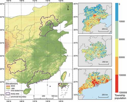
The study area of this dissertation includes the BTHR, Guangdong Province, and Guizhou Province (Figure 1). The BTHR is located at the center of the Bohai Sea economic circle; it includes Beijing, Tianjin, and Hebei Provinces, and is the most important population concentration area in northern China. The area is characterized by significant differences in the natural environment and a high degree of economic diversification (Xie, Yafen, and Xie 2017; Zhang et al. 2017). Guangdong Province is located at the southernmost point of mainland China and is the most populous province. The province’s topography is predominantly mountainous and hilly, with only 27.2% of the land classified as plains. Like the BTHR, the area includes both the most developed mega-city clusters in China and government-defined national poverty-stricken counties, each with markedly different economic conditions (Wu et al. 2017; Yang 2017). Guizhou Province is located in southwestern China. The province’s topography is dominated by plateaus and mountains, which account for 92.5% of the total area. The province is economically underdeveloped and contains the largest number of people living below China’s poverty line (Feng and Long 2019; Xu et al. 2020). The unique natural and economic characteristics of these regions have granted the study area a demographic profile with dense, even, and sparse population distribution patterns. These environmental, economic, and population differences help extend our study’s applicability to more scenarios.

Figure 1. Location of the study area and population distribution of the township.

2.2. Datasets

We used four main data types – preexisting primary maps, demographic data, ancillary data, and reference data – which are detailed in Table 1.

Table 1. Input datasets for multisource map fusion

Name	Year(s)	Spatial resolution	Address
GPW4	2015	30 arc-seconds	https://sedac.ciesin.columbia.edu/data/collection/gpw-v4/sets/browse
LandScan	2015	30 arc-seconds	https://landscan.ornl.gov/
WorldPop	2015	30 arc-seconds	https://www.worldpop.org/?tdsourcetag=s_pctim_aiomsg
Population sample survey data	2015	Township	https://data.cnki.net/
Demographic data	2005–2015	Village	http://fz.wanfangdata.com.cn/index.do
Impervious surfaces data	2015	30 m	http://data.ess.tsinghua.edu.cn/
Mobile phone positioning data	2015	0.01 decimal degree	https://heat.qq.com/

2.2.1. Primary population maps

The GPW collection, introduced by the Columbia University Center for International Earth Science Information Network (CIESIN), is the result of the Gridded Population of the World project. GPW4, the fourth version of the project, is currently the only global-scale population grid produced using the area-weighting approach. To ensure that the product exhibits relatively high accuracy, GPW4 uses the population of the lowest available administrative unit as the basic unit of modeling in the production process, which in China is the township level. Since GPW4 simply distributes the census population equally, its accuracy is lowest in most evaluations (Bustos et al. 2020). However, in areas where the population is evenly distributed, it may also reflect their real situation (Bai et al. 2018; Danchun et al. 2020).

LandScan is a global-scale spatial gridded population distribution dataset produced by Oak Ridge National Laboratory. It uses sub-national census data combined with various ancillary variables, such as land cover, roads, and slope, to complete the spatial grid of the census population based on multielement dasymetric mapping. Considering the differences in the importance of these variables under different regional geographic conditions, external intervention was used in the modeling process to make corresponding adjustments to the weighting. This method is also referred to as “intelligent interpolation” technology (Leyk et al. 2019). LandScan tends to underestimate the population more than other datasets, especially in urban areas and urban-rural transition areas (Calka and Bielecka 2019).

WorldPop is a global-scale gridded population mapping project led by a research team at the University of Southampton. Its production integrates the RF algorithm and dasymetric mapping. The RF algorithm is used to fit the relationship between several ancillary variables and population density to obtain a population distribution indicator layer; then, the indicator information obtained from this layer is used to complete the population distribution (Stevens, et al. 2015). Due to excellent modeling methods and more input variables, WorldPop’s accuracy is usually higher than other common datasets (Gaughan et al. 2016; de Mattos, McArdle, and Bertolotto 2020; Xu et al. 2021).

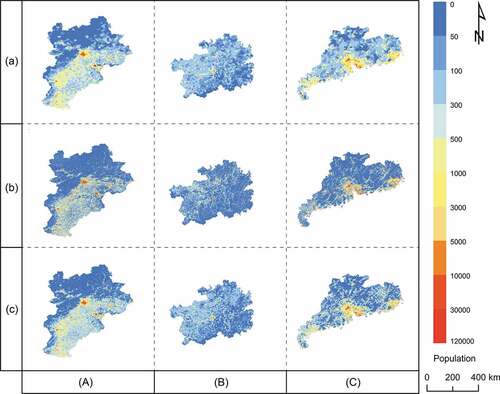
There are two main reasons for selecting the three aforementioned products: (1) they exhibit wide coverage, matching spatial resolution, and coincidence of time nodes, which are conducive to the processing of map fusion and further promotion; and (2) their modeling methods, modeling scales, and data sources are quite different, and they contain diverse population distribution information, which is conducive to the full utilization of the map fusion effect. Figure 2 shows the profiles of these products in the study area.

Figure 2. Distribution maps of the gridded population in the study area: (A) BTRG, (B) Guizhou Province, (C) Guangdong Province; (a) GPW4, (b) LandScan, and (c) WorldPop.

2.2.2. Demographic data

Multisource map fusion requires actual population data. For this purpose, we collected statistical data from the 2015 national 1% population sample survey, the sixth population census in 2010, and the demographic data from some villages from 2005 to 2015. Population sample surveys and censuses are national-scale survey programs led by the Chinese government and have an authority that cannot be ignored. They are reported at five levels: country, province, city, county, and township. In this study, we selected statistics at the township level to ensure the accuracy of the subsequent data processing results. These township data are dominated by the 2015 national sample data, but due to certain missing data in the study area, we adjusted the 2010 census data with the population growth rates of the higher administrative units and used it to supplement the missing data. Some village statistics were also collected, as not all of the township data met our requirements. The data were obtained from local chronicles, which are usually written by people who know these areas the well. As the local chronicles in the study area have not been systematically sorted, and many cannot provide accurate population counts, we had to expand the time range of the data to meet the required number of samples. This is why the time frame was set as 2005–2015. Although this time frame is relatively large, village data will mainly be used in rural areas, where population changes are relatively small, and we will further process to reduce the influence of the time difference.

2.2.3. Ancillary data

Impervious surfaces and mobile phone positioning data were used as ancillary variables in the additional fusion experiment conducted to test the effect of the additional information on the accuracy of the results and to construct reference data. Traditional ancillary data, such as elevation, slope, land use, and roads, require complex integration processes due to their weak population indication capabilities (Liu et al. 2018a; Yang et al. 2019), while commonly used nighttime lights also require a series of corrections due to their saturation and blooming effects (Levin and Duke 2012; Sahoo, et al. 2020; Tan et al. 2018). These two types of data are generally used to produce highly accurate population distribution maps because they provide a better representation of population distribution, are easily accessible, and better meet our need for the simple and efficient production of the reference data needed for map fusion (Azar et al. 2010; Chen et al. 2020a; Patel et al. 2017; Wei et al. 2020). The experiment used impervious surface data from 2010 at a 30 m resolution. These data were produced mainly based on LANDSAT images from the Google Earth Engine, which provides archival images from 1985 to 2018 (Gong et al. 2020). However, upon inspection, it was found that many houses in Guizhou province were not detected by the impervious surface data, which may be attributable to a unique local house structure that could not be captured by the corresponding algorithm. Therefore, the GHS_BUILT_S1NODSM_GLOBE_R2018A data generated based on deep learning and image recognition techniques were selected as a supplement, based on their suggestion to set a threshold of 0.2 to extract the population settlement layers that were not captured by the impervious surface data (Corbane et al. 2021). We masked the population settlement layer with 2018 impervious surface data to eliminate the effect of impervious surface expansion due to temporal differences, and the processed settlement data were merged into the 2015 impervious surface to fill in the missing information. Meanwhile, mobile phone location data are considered the most direct indicator for describing population distribution and are used in studies of short-term population migration and resident population distribution (Cheng, Wang, and Yong 2020; Pan and Lai 2019; Song, Chen, and Kwan 2020). According to the 2016 China Communications Yearbook report, the number of mobile phones used in China in 2015 was 93 per 100 people, 103 per 100 people in BTHR, 134 per 100 people in Guangdong Province, and 90 per 100 people in Guizhou Province. Mobile location data were obtained from Tencent, whose location-based services reach approximately 70% of the Chinese population; in some first-tier cities, this value can exceed 93% (Yao et al. 2017). We obtained Tencent location data for all of 2015 to attenuate the potential impact from population movement by means of a long time series.

2.2.4. Reference data

The reference data of the population count is the response variable in each fusion algorithm, and its accuracy is defined as the upper limit of achievable result accuracy; therefore, it plays a significant role throughout the experiment. However, it is very difficult to obtain the real population at the grid scale. Therefore, we propose a method for producing matching reference data based on data accessibility and population distribution.

2.2.4.1. Study area division

Due to the strong spatial heterogeneity of the population distribution in the study area, we first needed to delineate the distribution to use the reference data production methods adapted to the different population distribution profiles, thus improving accuracy. This division was based on the degree of population aggregation (Dou et al. 2018; Liu et al. 2010), which is an indicator that describes population distribution. This can be expressed as follows:

(1) $\begin{array}{c}PA{D}_i=\frac{P_i/A_i}{P_n/A_n}\end{array}$(1)

where $PA{D}_i$ represents the population concentration of township $i$, $P_i$ represents the population of township $i$, $A_i$ represents the land area of township $i$, $P_n$ represents the total population of the study area, and $A_n$ refers to the total study area. Based on the reality of the study area, we divided each area into the following three areas with agglomeration values of 2 and 0.5 as the cutoff points (Wang and Chen 2018), as follows: densely populated area, evenly populated area, and sparsely populated area.

2.2.4.2. Densely populated area

The production of reference data in this area was mainly based on mobile phone positioning data. First, the daily average of Tencent’s mobile phone positioning data in 2015 was calculated as stable positioning information. As the resolution of the positioning data was 0.01°, a bilinear method was used to resample the data to 30 arcsec to match their resolution with those of the population grids. Since location requests may be repeatedly recorded, we referred to He et al. (2020) for further processing. The thus-obtained grids of stable mobile phone positioning count in the study area were aggregated to the township scale, and the ratio of positioning counts within each grid to the total positioning counts in the township was calculated to obtain a weighted layer for population allocation. Then, according to this weighting layer, a township-level census was assigned to each grid from the top-down to obtain the reference data of densely populated area.

2.2.4.3. Evenly populated area

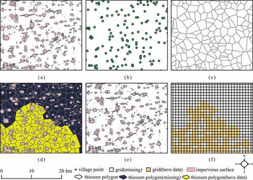
To get as close as possible to the real population distribution, impervious surface data and village demographics at the highest resolution available were used to produce reference data for the area. The preparation of the reference data for evenly populated area involved the following five main steps. (1) Collate the local chronicles from 2005 to 2015 to obtain village-level population data for the corresponding year. (2) Compare the township population recorded in the local chronicles with the 2010 census data to obtain the population change rate, which can be used to correct the time point difference in the village-level population. (3) According to the administrative division code, call the Baidu Map API to obtain the coordinates of all villages in evenly populated area and manually inspect the villages selected in (1). (4) Construct Tyson polygons using the village coordinate points as the base points to represent the village boundary (Dong et al. 2017; Liu et al. 2018b), and superimpose the impervious surfaces over these polygons to obtain the population and village name labels. Then, calculate the population density of the impervious surfaces. (5) Intersect the grids with the impervious surfaces, calculate the area of the impervious surfaces in each grid, and inversely calculate the population to obtain the reference population data of the evenly distributed area (Figure 3).

Figure 3. Approaches adopted for producing reference data for an evenly populated area. (a) Impervious surfaces at 30 m resolution, (b) village coordinates, (c) Tyson polygons, (d) Tyson polygons for which the population density information was obtained, (e) impervious surfaces with population density obtained after grid partitioning, and (f) reference data for the area with an even population distribution.

2.2.4.4. Sparsely populated area

The sparsely populated area mainly comprises highland and mountainous regions, where none of the above-described reference data production methods are applicable due to the harsh natural environment and poor economic conditions. At the same time, to the best of our knowledge, there is no production method for high-precision gridded population data for such an area, so no reference population data are available for this area.

The number of reference population data grids produced using the two methods described above was statistically aggregated to 13,162. By setting the population to exist only on impervious surfaces, the number of grids with population distribution in dense and even areas were 83,763, and the reference data represented 15.71% of the total population distribution grids. The reference data were randomly divided into calibration and validation data according to a 7:3 weighting.

2.3. Methodology

2.3.1. Generic framework

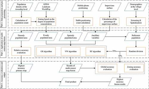
Figure 4 shows the general framework of multisource map fusion, which can be summarized in three parts and five steps. (1) Data collection and preprocessing: Unify all data to the World Geodetic System 1984, with a resolution of 30 arcsec, and use the Asia North Albers equal-area conic projection coordinate system for data calculation. (2) Relative accuracy evaluation: Use township census data to evaluate the relative accuracy of the three input gridded population maps in the area without reference data. (3) Implement the multisource map fusion algorithm; (4) followed by total and zoning-scale accuracy evaluations of the output results and the three input maps; and (5) combine the output result with the highest accuracy and part of the existing population map with the best relative accuracy to obtain the final product.

Figure 4. Framework for achieving multisource map fusion.

2.3.2. Fusion algorithms

2.3.2.1. GR algorithm

The GR algorithm, proposed by Granger and Ramanathan (1984), assumes a linear relationship between the products of different models and calibration data, which can be fitted by a multiple linear regression equation, with the regression equation coefficients being the weights of the corresponding products. The outcome $Y_{GR}\left(s\right)$ of the GR algorithm can be calculated as

(2) $\begin{array}{c}{Y}_{GR}\left(s\right)=\sum _{i=1}^p\left({\beta }_i\hspace{0.17em}{X}_i\left(s\right)\right)+{\beta }_0\end{array}$(2)

where ${\beta }_i$ and $p$ are the weights and quantities of the input data, respectively; ${\beta }_0$ is the intercept, and $X_i\left(s\right)$ and $Y_{GR}\left(s\right)$ are the population counts for input data $i$ and calibration data at position $s$. As the input data exhibited strong covariance (variance inflation factor > 10), ridge regression was used to solve the equation. The fusion of the GR algorithm was attempted in two cases: Case 1, which included only the three original maps, and Case 2, which had two extra variables – ISP and NP – in addition to the original maps. The variable $p$ in formula (2) was assigned the values of 3 and 5 for Cases 1 and 2, respectively.

2.3.2.2. VW algorithm

The VW algorithm is an extension of the Bates-Granger algorithm (Bates and Granger 1969; Ge et al. 2014; Heuvelink and Bierkens 1992) and involves two main steps: deviation removal and weighted linear averaging of the input data. The weight is derived from the uncertainty between the calibration data and input data, expressed as the variance and covariance between them. To ensure accuracy, the algorithm adopts the strategy of partition modeling and can further use the partition extrapolation results to fill in some areas with missing data. This can be expressed as follows:

(3) $\begin{array}{c}{Y}_{vw}\left(s\right)=\sum _{i=1}^p{\beta }_i\hspace{0.17em}\left(X_i\left(s\right)-v_i\left(s\right)\right)\end{array}$(3)

where $Y_{vw}\left(s\right)$ represents the output population at $s$; ${\beta }_i$ and $p$ are the weight and quantity of the input data, respectively; and $X_i\left(s\right)$ and $v_i\left(s\right)$ are the population counts and bias of input data $i$ at $s$. The bias calculation can be expressed as

(4) $\begin{array}{c}{\hat{v}}_i=\frac{1}{n}\sum _{s=1}^n\left(X_i\left(s\right)-y\left(s\right)\right)\end{array}$(4)

where ${\hat{v}}_i$ is the bias of input data $i$; $X_i\left(s\right)$ and $y\left(s\right)$ represent the population counts of input data $i$ and calibration data at $s$, respectively; and $n$ is the number of calibration points.

The input weight vector $\beta$ for the different maps can be calculated by minimizing the variance of the estimation error of the fusion results:

(5) $\begin{array}{c}\beta {\left(s\right)}^T={\left(1^T\mathbf{C}{\left(s\right)}^{-1}1\right)}^{-1}{1}^T\mathbf{C}{\left(s\right)}^{-1}\end{array}$(5)

where 1 represents a $p$-dimensional unit vector and $\mathbf{C}\left(s\right)$ is the variance-covariance matrix representing the error, which can be calculated as

(6) $\begin{array}{c}{\stackrel{⌢}{C}}_{ij}=\frac{1}{n}\sum _{s=1}^n\left(X_i\left(s\right)-y\left(s\right)\right)\left(X_j\left(s\right)-y\left(s\right)\right)\end{array}$(6)

where $i$,$\hspace{0.17em}j=1$, …,$\hspace{0.17em}p$ represents the data entered for the different gridded population distributions.

To ensure the accuracy of the algorithm and the representativeness of the calibration data, we divided the evenly distributed area into a number of different subzones according to the ISP within the grid using natural breaks. There are four in the BTHR (I, II, III, IV), three in Guangdong Province (I, II, III), and two in Guizhou Province (I, II). The densely populated area was divided into two subzones, according to the NP, using natural breaks.

2.3.2.3 RF algorithm

RF is a nonlinear and nonparametric modeling method proposed by Breiman (2001), which belongs to the “integrated learning” category. It combines generated single trees into a forest using the “bagging” method, which reserves the best combination of randomly selected variables for each node of each tree and outputs the final prediction by averaging the predictions of single trees:

(7) $\begin{array}{c}{Y}_{RF}\left(s\right)=\frac{1}{K}\sum _{k=1}^K{Y}_k\left(s\right)\end{array}$(7)

where $Y_{RF}\left(s\right)$ represents the regression prediction of the RF at $s$, $K$ represents the number of trees in the forest, and $Y_k\left(s\right)$ indicates the population predicted by the $k^{th}$ tree at $s$. Like the GR algorithm, the fusion attempts of the RF algorithm are also classified into Case 1, which contains only three original maps, and Case 2, which contains two ancillary variables and three maps.

2.3.3. Validation

To assess the utility of the fusion model, the remaining data in the reference dataset that were not used for calibration need to be used for evaluation. For to different purposes, we selected root mean squared error (RMSE), mean absolute error (MAE), and relative error (RE) as the accuracy evaluation metrics. RE is used to measure the similarity of available population products against census values at the township scale. MAE is used to measure the total deviation of the predicted values and RMSE is used to measure the accuracy of the prediction.

(8) $\begin{array}{c}RMSE=\sqrt{\frac{1}{n}\sum _{i=1}^n{\left({\hat{z}}_i-z_i\right)}^2}\end{array}$(8)

(9) $\begin{array}{c}MAE=\frac{1}{n}\sum _{i=1}^n\left|{\hat{z}}_i-z_i\right|\end{array}$(9)

(10) $\begin{array}{c}RE=\frac{\left|{\hat{z}}_i-z_i\right|}{z_i}\hspace{0.17em}100\mathrm{\%}\end{array}$(10)

where $n$ represents the number of validation grids, ${\hat{z}}_i$ is the population count estimated by the algorithm, and $z_i$ is its true value.

3. Results

3.1. Evaluation of sparsely populated area

Due to the lack of valid calibration data for a sparsely populated area, the relative accuracy of the gridded population maps was assessed by upscaling the grid-scale population to townships for comparison with census data. For this purpose, a gridded population map with relatively high accuracy and wide coverage was primarily considered to participate in the synthesis of the final product; thus, a RE with an acceptable lower limit of 50% was chosen as the metric. As shown in Table 2, in a sparsely populated area, WorldPop has a significant advantage over other maps in terms of its high-accuracy coverage. The areas that meet the accuracy requirements account for 86.32% of the entire sparsely populated area in BTHR, 83.49% in Guangdong Province, and 95.04% in Guizhou Province. In addition, the RE is 0 ~ 10% and 10 ~ 30% of the high-precision area; WorldPop’s area percentage is also better than the other two products, whether in BTHR, Guangdong Province, or Guizhou Province. Therefore, WorldPop was selected as the representative data for the sparsely populated area.

Table 2. Percentage of townships for multiple input maps with different relative error ranges

Area	Name	Relative error
		0–10%	10%-30%	30%-50%	Total
BTHR	GPW4	22.45%	42.32%	16.39%	81.16%
	LandScan	16.13%	30.32%	24.00%	70.45%
	WorldPop	26.58%	43.61%	16.13%	86.32%
Guangdong Province	GPW4	24.01%	37.93%	18.69%	80.63%
	LandScan	15.83%	30.97%	21.56%	68.35%
	WorldPop	24.69%	41.75%	17.05%	83.49%
Guizhou Province	GPW4	30.53%	43.51%	18.32%	92.37%
	LandScan	14.12%	25.95%	26.34%	66.41%
	WorldPop	30.15%	46.18%	18.70%	95.04%

Note. Input the number of townships within different relative error intervals on the map as a proportion of the total number of townships in the sparsely populated area.

3.2. Evaluation of densely and evenly populated areas

To investigate the effectiveness of zonal modeling, evaluations for evenly and densely populated areas were conducted using both total and zonal perspectives, with site zoning divided according to the number of subzones in the VW algorithm. For each zone, the RMSE and MAE values of the input gridded population maps and the output results were calculated from the validation data. At the total scale, in addition to using the above-described evaluation metrics, we also used the Taylor diagram to compare the differences in accuracy between the input maps and output results.

3.2.1. Subzone evaluation

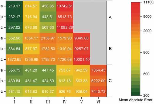
As shown in Figure 5 and Figure 6, the RMSE and MAE values of the GR algorithm and the RF algorithm are significantly different in various subzones. For RMSE, in Guizhou Province, the GR algorithm has higher values in zones I (344.74) and IV (16,738.15) than the RF algorithm in the corresponding partition (337.64) (14,558.19); similarly, in Guangdong Province, the GR algorithm is higher in zones I (1486.83) and V (17,153.19) than the corresponding 895.59 and 15,433.24 of the RF algorithm. In BTHR, the GR algorithm is lower than the RF algorithm only in zones IV (1254.44) and V (1593.35), and is higher than the corresponding value of RMSE for the RF algorithm in all other subzones. For MAE, the GR and RF algorithms still correspond to RMSE in the two endpoint subzones of BTHR, Guizhou Province and Guangdong Province, with the GR algorithm remains higher than the RF algorithm. The difference is that the number of subzones where the GR algorithm is higher than the RF algorithm increases, such as zone III in Guizhou Province, zone IV in BTHR and Guangdong Province. In most subzones of BTHR, Guizhou Province and Guangdong Province, the values of the VW algorithm are significantly lower than the other two algorithms in both RMSE and MAE.

Figure 5. Heat map representing the root-mean-squared error of different algorithms (a for RF algorithm, b for VW algorithm, c for GR algorithm; A refers to Guizhou Province, B is Guangdong Province, and C is BTHR).

Note. The VW algorithm refers to the variance weighted algorithm; GR algorithm is the Granger-Ramanathan algorithm; RF algorithm denotes the random forest algorithm.

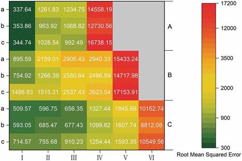
Figure 6. Heat map representing the mean absolute error of different algorithms (a for RF algorithm, b for VW algorithm, c for GR algorithm; A refers to Guizhou Province, B is Guangdong Province, and C is BTHR).

Note. The VW algorithm refers to the variance weighted algorithm; GR algorithm is the Granger-Ramanathan algorithm; RF algorithm denotes the random forest algorithm.

3.2.2. Total evaluation

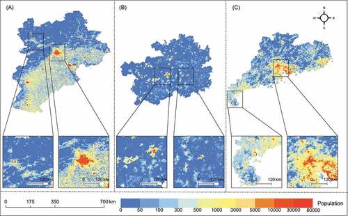
Table 3 reports the accuracy performance of the input gridded population maps and the map fusion outputs from the total perspective. The RMSE and MAE of the input population maps are similar to those reported in existing studies, with WorldPop showing the highest accuracy. The majority of the fusion results have substantially reduced RMSE and MAE values compared to the input prime maps. Among them, compared with the input map with the lowest accuracy, the RMSE and MAE of the fusion map are reduced by a maximum of 24.88% and 32.62% in BTHR, 28.44% and 35.88% in Guangdong Province, and 16.40%and 20.88% in Guizhou Province Compared to the input map with the highest accuracy, these values change were 13.66% and 20.39%, 15.47% and 18.29%, and 5.05% and 6.15%. When map fusion algorithms were applied to gridded population maps only, the VW algorithm reported the lowest RMSE and MAE values in BTHR, Guangdong Province, and Guizhou Province, where the RMSE was 2469.12, 4810.89, and 2008.07, and the MAE was 958.43, 1816.08, and 562.70. When ancillary variables are involved in each map fusion algorithm, the percentage reductions of RMSE and MAE for the GR algorithm were 6.70% and 16.08% (BTRH), 9.34% and 22.17% (Guangdong Province), and 11.08% and 16.03% (Guizhou Province), while the corresponding values for the RF algorithm were 9.57% and 19.93%, 14.60% and 25.16%, and 7.39% and 17.36%. The RF algorithm has the lowest RMSE and MAE in Guangdong Province, but the RMSE in BTHR and Guizhou Province is slightly higher with 2569.67 and 2130.30 than 2469.12 and 2008.07 for the VW algorithm. Among the three areas, the map fusion algorithm had the least reduction in RMSE and MAE in Guizhou province, with a reduction ratio of only 5.05% and 6.15%, respectively, compared to the most accurate input map. Figure 7 shows that the accuracy of the different input maps and fused maps gradually improves as the reference point with coordinates (1, 0) is gradually approached (Taylor 2001). The highest accuracy reported for all areas is the result of multisource map fusion, with the RF algorithm for Guangdong Province and the VW algorithm for both BTHR and Guizhou Province. Thus, these corresponding results will be stitched together with the most accurate WorldPop data for sparsely populated area into an output product that can finally be used (Figure 8).

Table 3. Evaluation indicator values reported for different data in a total perspective

Area	BTHR			Guangdong		Guizhou
Name	RMSE		MAE	RMSE	MAE	RMSE	MAE
GPW4	2980.35	1098.92		5700.71	2194.98	2402.07	651.09
LandScan	3287.09	1257.21		6296.72	2443.01	2282.40	711.22
WorldPop	2859.71	1064.21		5330.00	1917.32	2114.98	542.53
VW algorithm	2469.12	958.43		4810.89	1816.08	2008.07	562.70
GR algorithm Case 1	2895.09	1197.84		5593.11	2351.01	2498.51	672.42
RF algorithm Case 1	2841.56	1057.99		5275.79	2093.17	2300.35	616.08
GR algorithm Case 2	2701.06	1005.27		5070.48	1829.90	2221.68	564.61
RF algorithm Case 2	2569.67	847.17		4505.62	1566.58	2130.30	509.14

Note. RMSE refers to root mean squared error; MAE is mean absolute error; VW algorithm refers to the variance weighted algorithm; GR algorithm is the Granger-Ramanathan algorithm; RF algorithm denotes the random forest algorithm; Case 1 is map fusion for the input maps only; Case 2 adds two ancillary variables to Case 1.

Figure 7. Taylor diagram describing the overall accuracy of the different data. Note. A: GPW4, B: LandScan, C: WorldPop, D: Variance weighted algorithm, E: Granger-Ramanathan algorithm with Case 1, F: Random forest algorithm with Case 1, G: Granger-Ramanathan algorithm with Case 2, H: Random forest algorithm with Case 2; a: BTHR, b: Guizhou Province, c: Guangdong Province.

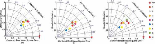
Figure 8. Final output: The most accurate fusion result is spliced with WorldPop in the sparsely populated area (A: BTHR, B: Guizhou Province, C: Guangdong Province).

4. Discussion

4.1. Weights for primary maps and ancillary variables

Table 4 reports the relative importance of different variables in various areas, using the RF algorithm as representative. In the fusion attempt using only the primary maps, WorldPop reported the highest importance in almost all situations. With the addition of ancillary variables, the importance of the primary maps decreased, and NP became the highest-weighted variable, whereas ISP’s importance was much lower than NP’s importance.

Table 4. Relative importance of different variables for the RF algorithm in BTHR, Guangdong Province, and Guizhou Province

Name	RF algorithm Case 1			RF algorithm Case 2
	BTHR	Guangdong	Guizhou	BTHR	Guangdong	Guizhou
GPW4	30%	27%	27%	14%	15%	20%
LandScan	33%	28%	33%	15%	16%	17%
WorldPop	38%	45%	40%	22%	24%	32%
ISP				6%	6%	4%
NP				42%	39%	27%

Note. The GR algorithm refers to the Granger-Ramanathan algorithm; the RF algorithm denotes the random forest algorithm; ISP is the impervious surface percentage; and NP represents the number of mobile phone positionings. The numbers in the table indicate the importance of the variables.

The differences in the importance of the primary maps are mainly attributed to their modeling methods and different input data. WorldPop is significantly more important than the other two gridded population maps due to its more comprehensive modeling techniques. According to the values of zoning weights for the different population maps, WorldPop reports the best results in both the less populated Guizhou Province and the more populated Guangdong Province due to the many-dimensional ancillary variables, which gives the model greater generalizability. The importance of LandScan in all areas is lower than that of WorldPop, indicating that population modeling at large scales, such as the sub-national level, tends to ignore local spatial variation, leading to large differences in modeling results at the grid scale and in the calibration data. GPW4 has lower importance than WorldPop and LandScan in all areas, but its comparatively higher importance in areas with relatively wide population distribution, such as BTHR and Guangdong Province, indicates the effectiveness of its unique modeling approach in homogeneous population area.

When ancillary variables were added to the GR and RF algorithms, the weight of the input gridded population maps was reduced, which we hypothesize is mainly because some of the information in the calibration data was derived from ancillary variables, resulting in the ISP and NP feeding back a stronger indication of population distribution. However, it is worth noting that ISP, which is also an ancillary variable, is significantly less important than NP, while the amount of calibration data produced according to the impervious surfaces is much greater than the positioning count. Considering that none of the positioning count variables were used in the primary maps modeling, it indicates that the main reason for the large proportion of NP is their new information with a strong population indication.

4.2. Performance evaluation of map fusion algorithms

The majority of the multisource map fusion algorithms positively impacted the accuracy of the gridded population maps, with the accuracy of the final output significantly better than that any of the three input maps alone. Viewed through a zoned perspective, as global regression classes of fusion algorithms, RF and GR have lower accuracy than the VW algorithm in almost all subzones. This is mainly due to the strong heterogeneity of the population distribution, which makes it difficult to obtain well-fitting results from the whole, and the neglect of local variation is a disadvantage of both algorithms. Furthermore, due to regional differences in the accuracy of the different input products, the effectiveness of the two regression algorithms differs (Chen et al. 2020b). The accuracy of the RF algorithm is higher than that of the GR algorithm in both the sparsely populated zone I and the densely populated zones IV, V, or VI (the most densely populated zones in the three different areas), indicating that the nonlinear RF algorithm is more suitable for modeling the relationship between the input map and the real population in cases of extreme population distribution. This would be attributed to the specificity of such extreme zones, where the predicted population of most existing models varies greatly, with complex correspondence and low accuracy. On the other hand, the GR algorithm is suitable for areas with evenly distributed populations, where the population distribution varies gently and the abundance of input data allows the different models to be fully effective, resulting in a predicted population that is close to the real population in most existing maps, and the relationship between them can be captured using a simple linear method alone.

The results of the total view validate the evaluation of the zonal scale, and the accuracy of the VW algorithm without the participation of ancillary variables is still higher than that of the RF and GR algorithms. When ancillary variables are added to both the GR and RF algorithms, the accuracy of both is further improved, but the RF algorithm improves more than the GR algorithm, indicating the potential for adding ancillary variables to perform fusion algorithm extensions. However, it is worth noting that although the improvement in accuracy resulting from the extension of the RF algorithm by adding ancillary variables is substantial, the reduction in RMSE is less than that of MAE, which means that the ability to handle the extreme values of the error is limited.

The effect of the multisource map fusion algorithm is lowest in Guizhou Province compared to the other two areas, which may be attributable to multiple reasons. On one hand, the population of the area is sparse, but the variation in the distribution is dramatic, which amplifies the effect of the differences of the values on the grid. On the other hand, the prediction results of the existing input maps in sparsely populated area are unsatisfactory (Calka and Bielecka 2019; de Mattos, McArdle, and Bertolotto 2020), where the uncertainties are passed through the fusion algorithm to the output results, and the small amount of reference data for calibration leads to an inability to fully exploit the effect. The VW algorithm may be an effective way to deal with this problem, and the use of zonal modeling reduces the need for calibration data in the same population distribution status zone, a suggestion that can be demonstrated by the comprehensive evaluation of the accuracy of the Taylor diagram of Guizhou Province.

The Taylor diagram synthetically selected the products with the highest accuracy among the three areas, which are the results of the VW algorithm in BTHR and Guizhou Provinces, and the results of the RF algorithm in Guangdong Province, which shows that the multisource map fusion algorithm is effective. The grid-based modeling approach makes it possible to overcome the uncertainty caused by most top-down modeling approaches in assigning populations at the township, county, and city scales (Leyk et al. 2019; Danchun et al. 2020), and gives the results of accuracy evaluation at the grid scale (Bai et al. 2018). At the same time, the integration of superior information from multiple source maps in different areas makes it possible to obtain a large scope of high-quality output, which is not possible with the bottom-up approach (Wardrop et al. 2018). The multisource map fusion algorithm can be effective without ancillary data, but integrating high-quality ancillary data, especially data not involved in existing product modeling, can further improve its effectiveness, as evidenced by the highest accuracy output obtained by the RF algorithm fusing mobile phone positioning data in Guangdong Province.

4.3. Limitations of multisource map fusion

4.3.1. Limitations of reference data

As sufficient real values of the grid population could not be obtained, we randomly divided the reference data into calibration and validation data. While this may lead to a correlation between the calibration and validation data, the accuracy of the output depends on that of the calibration data. In addition, because we used the highest-resolution, village-level statistical population and location data that highly correlated with the population available in the production of the reference data, their accuracy was reliable. At the same time, we used both top-down and bottom-up modeling perspectives based on data characteristics, representing the way in which most gridded population maps are produced. Therefore, the outputs are closer to the validation values than the input population maps, which indicates the effectiveness of map fusion in this field.

4.3.2. Uncertainty analysis

The uncertainties introduced in the experiments mainly originated from the primary maps and calibration data. The primary maps have differences in uncertainty due to differences in the input data and modeling methods, and the calibration data are used with the aim of reducing these uncertainties. However, as the calibration data are a finite sample, the uncertainties in the primary maps cannot be completely eliminated. Moreover, as standard calibration data, although we used the best variables available and modeling methods appropriate for the different regions, they are not truly representative of the real population, and their uncertainty will propagate to the output results. If the transmission of these uncertainties could be quantified, it would likely be a useful extension to this study.

5. Conclusions

Currently, although multiple population distribution maps are available, their modeling methods and superior information vary considerably. To address this issue, we propose an uncertainty-based fusion method for multisource population maps. Case studies conducted in different areas of China yielded the following results. First, the output accuracy of most fusion algorithms is higher than that of all input gridded population maps, and multisource map fusion of populations is effective. Second, the GR algorithm, as a simple global linear fusion algorithm, has limited effectiveness in fusing existing population maps alone. Third, the zoning modeling strategy of the VW algorithm is effective, and it should be the first fusion algorithm considered in the case of insufficient calibration data. Fourth, by adding ancillary variables, the accuracy of the map fusion results can be improved, especially when the corresponding ancillary variables are not involved in the modeling of the input maps. Fifth, compared to other algorithms, the nonlinear RF algorithm can be more adequately coupled to ancillary variables to achieve a more significant accuracy gain. This algorithm can be given preference when excellent ancillary variables are available. In conclusion, compared to the existing gridded population mapping method, the proposed multisource map fusion-based mapping method is simpler, more effective, and less expensive. This method is ideal for economically challenged countries and can help them obtain a large range of high-precision population products with a small survey of population, where further improvements in accuracy can be achieved by adding the appropriate auxiliary variables to suit their conditions.

In addition, multisource map fusion would ideally require actual population distribution data; however, due to the limitations of data availability, we independently produced reference data to replace these data and randomly divided them into calibration and validation data, which may lead to non-independence between them. Therefore, it will remain an important study direction to obtain sufficient and accurate population distribution data. This may involve issues such as the definition of “sufficient,” the distribution of population samples, and the trade-off between accuracy and cost. Meanwhile, the quantification of uncertainty in the overall fusion process may be another challenging research direction for the future.

Acknowledgements

This work was supported by the Strategic Priority Research Program of Chinese Academy of Sciences under Grant XDA20030302; National Natural Science Foundation for Distinguished Young Scholars of China under Grant 41725006; Key Research and Development Program of Shaanxi under Grant 2021NY-170; and Fundamental Research Funds for the Central Universities, CHD under Grant 300102120201. Authors would like to thank the organizations and individuals who provided publicly accessible data. Author would also like to thank the anonymous reviewers for their time and effort to review and improve this work.

Data availability statement

The data and codes that support the findings of this study are openly available in [figshare] at [https://www.doi.org/10.6084/m9.figshare.14740272].

Disclosure statement

No potential conflict of interest was reported by the author(s).

Additional information

Funding

This work was supported by the Strategic Priority Research Program of Chinese Academy of Sciences under Grant XDA20030302; National Natural Science Foundation for Distinguished Young Scholars of China under Grant 41725006; Key Research and Development Program of Shaanxi under Grant 2021NY-170; and Fundamental Research Funds for the Central Universities, CHD under Grant 300102120201.

References

- Azar, D., J. Graesser, R. Engstrom, J. Comenetz, R. M. Leddy, N. G. Schechtman, and T. Andrews, et al. 2010. “Spatial Refinement of Census Population Distribution Using Remotely Sensed Estimates of Impervious Surfaces in Haiti.” International Journal of Remote Sensing 31 (21): 5635–5655. doi:10.1080/01431161.2010.496799.
- Bai, Z., J. Wang, M. Wang, M. Gao, and J. Sun. 2018. “Accuracy Assessment of Multi-Source Gridded Population Distribution Datasets in China.” Sustainability 10 (5). doi:10.3390/su10051363.
- Bates, J. M., and C. W. J. Granger. 1969. “The Combination of Forecasts.” Journal of the Operational Research Society 20 (4): 451–468. doi:10.2307/3008764.
- Breiman, L. 2001. “Random Forests.” Machine Learning 45 (1): 5–32. doi:10.1023/A:1010933404324.
- Bustos, M. F. A., O. Hall, T. Niedomysl, and U. Ernstson. 2020. “A Pixel Level Evaluation of Five Multitemporal Global Gridded Population Datasets: A Case Study in Sweden, 1990–2015.” Population and Environment 1–23. doi:10.1007/s11111-020-00360-8.
- Calka, B., and E. Bielecka. 2019. “Reliability Analysis of LandScan Gridded Population Data. The Case Study of Poland.” ISPRS International Journal of Geo-Information 8 (5): 222. doi:10.3390/ijgi8050222.
- Cees, G. H., and J. A. Vrugt; Diks. 2010. “Comparison of Point Forecast Accuracy of Model Averaging Methods in Hydrologic Applications.” Stochastic Environmental Research and Risk Assessment 24 (6): 809–820. doi:10.1007/s00477-010-0378-z.
- Chen, R., H. Yan, F. Liu, D. Wenpeng, and Y. Yang . 2020a. “Multiple Global Population Datasets: Differences and Spatial Distribution Characteristics.” ISPRS International Journal of Geo-Information 9 (11). doi:10.3390/ijgi9110637.
- Chen, S., V. L. Mulder, G. B. M. Heuvelink, L. Poggio, M. Caubet, M. R. Dobarco, C. Walter, and D. Arrouays, et al. 2020b. “Model Averaging for Mapping Topsoil Organic Carbon in France.” Geoderma 366. doi:10.1016/j.geoderma.2020.114237.
- Cheng, Z., J. Wang, and G. Yong. 2020. “Mapping Monthly Population Distribution and Variation at 1-km Resolution across China.” International Journal of Geographical Information Science 1–19. doi:10.1080/13658816.2020.1854767.
- Corbane, C., V. Syrris, F. Sabo, P. Politis, M. Melchiorri, M. Pesaresi, P. Soille, and T. Kemper, et al. 2021. “Convolutional Neural Networks for Global Human Settlements Mapping from Sentinel-2 Satellite Imagery.” Neural Computing & Applications 33.12 (12): 6697–6720. doi:10.1007/s00521-020-05449-7.
- Danchun, L., M. Tan, K. Liu, L. Liu, and Y. Zhu. 2020. “Accuracy Comparison of Four Gridded Population Datasets in Guangdong Province, China.” Tropical Geography 40 (2): 346–356. doi:10.13284/j.cnki.rddl.003220.
- de Mattos, A. C., G. McArdle, and M. Bertolotto. 2020. “Assessing the Quality of Gridded Population Data for Quantifying the Population Living in Deprived Communities.” arXiv Preprint arXiv:2011.12923.
- Dmowska, A., and T. F. Stepinski. 2017. “A High Resolution Population Grid for the Conterminous United States: The 2010 Edition.” Computers, Environment and Urban Systems 61: 13–23. doi:10.1016/j.compenvurbsys.2016.08.006.
- Dobarco, R., D. A. Mercedes, P. Lagacherie, R. Ciampalini, and N. P. A. Saby. 2017. “Prediction of Topsoil Texture for Region Centre (France) Applying Model Ensemble Methods.” Geoderma 298: 67–77. doi:10.1016/j.geoderma.2017.03.015.
- Dong, N., X. Yang, H. Cai, and D. Huang. 2017. “Suitability Evaluation of Gridded Population Distribution: A Case Study in Rural Area of Xuanzhou District, China.” Acta Geographica Sinica 72 (12): 2310–2324. doi:10.11821/dlxb201712014.
- Dou, X., J. Song, L. Wang, B. Tang, X. Shaofeng, F. Kong, and X. Jiang, et al. 2018. “Flood Risk Assessment and Mapping Based on a Modified Multi-parameter Flood Hazard Index Model in the Guanzhong Urban Area, China.” Stochastic Environmental Research and Risk Assessment 32 (4): 1131–1146. doi:10.1007/s00477-017-1429-5.
- Doxsey-Whitfield, E., S. B. Kytt Macmanus, L. P. Adamo, J. Squires, O. Borkovska, and S. R. Baptista. 2015. “Taking Advantage of the Improved Availability of Census Data: A First Look at the Gridded Population of the World, Version 4.” Papers in Applied Geography 1 (3): 226–234. doi:10.1080/23754931.2015.1014272.
- Feng, Y., and H. Long. 2019. “The Mechanism and Countermeasures of Solving Spatial Poverty Based on Rural Population Transfer and Rural Road Construction: A Case Study of Guizhou Province.” Geographical Research 38 (11): 2606–2623. doi:10.11821/dlyj020181397.
- Fletcher, D. 2019. Model Averaging. Berlin: Springer. doi:10.1007/978-3-662-58541-2.
- Gaughan, Andrea E., Forrest R. Stevens, Zhuojie Huang, Jeremiah J. Nieves, Alessandro Sorichetta, Shengjie Lai, Xinyue Ye , et al. 2016.“Spatiotemporal patterns of population in mainland China, 1990 to 2010.“ Scientific Data 3(1): 1–11. doi:10.1038/sdata.2016.5.
- Ge, Y., V. Avitabile, G. B. M. Heuvelink, J. Wang, and M. Herold. 2014. “Fusion of Pan-tropical Biomass Maps Using Weighted Averaging and Regional Calibration Data.” International Journal of Applied Earth Observation and Geoinformation 31: 13–24. doi:10.1016/j.jag.2014.02.011.
- Gong, P., L. Xuecao, J. Wang, Y. Bai, B. Chen, H. Tengyun, X. Liu, et al. 2020. “Annual Maps of Global Artificial Impervious Area (GAIA) between 1985 and 2018.” Remote Sensing of Environment 236. doi:10.1016/j.rse.2019.111510.
- Granger, C. W. J., and R. Ramanathan. 1984. “Improved Methods of Combining Forecasts.” Journal of Forecasting 3 (2): 197–204. doi:10.1002/for.3980030207.
- Hagedorn, R., F. J. Doblas-Reyes, and T. N. Palmer. 2005. “The Rationale behind the Success of Multi-model Ensembles in Seasonal forecasting—I. Basic Concept.” Tellus A: Dynamic Meteorology and Oceanography 57 (3): 219–233. doi:10.3402/tellusa.v57i3.14657.
- Hay, S. I., A. M. Noor, A. Nelson, and A. J. Tatem. 2005. “The Accuracy of Human Population Maps for Public Health Application.” Tropical Medicine & International Health: TM & IH 10 (10): 1073–1086. doi:10.1111/j.1365-3156.2005.01487.x.
- He, H., Y. Shen, C. Jiang, T. Li, M. Guo, and L. Yao. 2020. “Spatiotemporal Big Data for PM2. 5 Exposure and Health Risk Assessment during COVID-19.” International Journal of Environmental Research and Public Health 17.20 (20): 7664. doi:10.3390/ijerph17207664.
- Heuvelink, G. B. M., and M. F. P. Bierkens. 1992. “Combining Soil Maps with Interpolations from Point Observations to Predict Quantitative Soil Properties.” Geoderma 55 (1–2): 1–15. doi:10.1016/0016-7061(92)90002-O.
- Hjort, N. L., and G. Claeskens. 2003. “Frequentist Model Average Estimators.” Journal of the American Statistical Association 98 (464): 879–899. doi:10.1198/016214503000000828.
- Huang, X., C. Wang, L. Zhenlong, and H. Ning. 2020. “A 100 M Population Grid in the CONUS by Disaggregating Census Data with Open-source Microsoft Building Footprints.” Big Earth Data 5 (1): 112–133. doi:10.1080/20964471.2020.1776200.
- Huang, X., D. Zhu, F. Zhang, T. Liu, L. Xiao, and L. Zou. 2021. “Sensing Population Distribution from Satellite Imagery via Deep Learning: Model Selection, Neighboring Effect, and Systematic Biases.” IEEE Journal of Selected Topics in Applied Earth Observations and Remote Sensing 14: 5137–5151. doi:10.1109/JSTARS.2021.3076630.
- Jia, P., Y. Qiu, and A. E. Gaughan. 2014. “A Fine-scale Spatial Population Distribution on the High-resolution Gridded Population Surface and Application in Alachua County, Florida.” Applied Geography 50: 99–107. doi:10.1016/j.apgeog.2014.02.009.
- Levin, N., and Y. Duke. 2012. “High Spatial Resolution Night-time Light Images for Demographic and Socio-economic Studies.” Remote Sensing of Environment 119: 1–10. doi:10.1016/j.rse.2011.12.005.
- Leyk, S., A. E. Gaughan, S. B. Adamo, D. S. Alex, D. Balk, S. Freire, A. Rose, et al. 2019. “The Spatial Allocation of Population: A Review of Large-scale Gridded Population Data Products and Their Fitness for Use.” Earth System Science Data 11 (3): 1385–1409. doi:10.5194/essd-11-1385-2019.
- Liu, L., Z. Peng, H. Wu, H. Jiao, and Y. Yu. 2018a. ““Exploring Urban Spatial Feature with Dasymetric Mapping Based on Mobile Phone Data and LUR-2SFCAe Method.” Sustainability 10 (7): 2432. doi:10.3390/su10072432.
- Liu, R., Z. Feng, Y. Yang, and Z. You. 2010. “Research on the Spatial Pattern of Population Agglomeration and Dispersion in China.” Progress in Geography 29 (10): 1171–1177. doi:10.11820/dlkxjz.2010.10.003.
- Liu, Z., M. Ting, D. Yunyan, T. Pei, Y. Jiawei, and H. Peng. 2018b. “Mapping Hourly Dynamics of Urban Population Using Trajectories Reconstructed from Mobile Phone Records.” Transactions in GIS 22 (2): 494–513. doi:10.1111/tgis.12323.
- Lu, D., Y. Wang, Q. Yang, S. Kangchuan, H. Zhang, and L. Yuanqing. 2021. “Modeling Spatiotemporal Population Changes by Integrating DMSP-OLS and NPP-VIIRS Nighttime Light Data in Chongqing, China.” Remote Sensing 13 (2). doi:10.3390/rs13020284.
- Malone, B. P., B. Minasny, N. P. Odgers, and A. B. McBratney. 2014. “Using Model Averaging to Combine Soil Property Rasters from Legacy Soil Maps and from Point Data.” Geoderma 232-234: 34–44. doi:10.1016/j.geoderma.2014.04.033.
- Mennis, J. 2003. “Generating Surface Models of Population Using Dasymetric Mapping.” The Professional Geographer 55 (1): 31–42. doi:10.1111/0033-0124.10042.
- Moral-Benito, E. 2015. “Model Averaging in Economics: An Overview.” Journal of Economic Surveys 29 (1): 46–75. doi:10.1111/joes.12044.
- Noi, P., J. Degener, and M. Kappas. 2017. “Comparison of Multiple Linear Regression, Cubist Regression, and Random Forest Algorithms to Estimate Daily Air Surface Temperature from Dynamic Combinations of MODIS LST Data.” Remote Sensing 9 (5). doi:10.3390/rs9050398.
- Pan, Jinghu, and Jianbo Lai. 2019.“Spatial pattern of population mobility among cities in China: Case study of the National Day plus Mid-Autumn Festival based on Tencent migration data“ Cities 94:55–69. doi: 10.1016/j.cities.2019.05.022.
- Patel, N. N., F. R. Stevens, Z. Huang, A. E. Gaughan, I. Elyazar, and A. J. Tatem. 2017. “Improving Large Area Population Mapping Using Geotweet Densities.” Transactions in GIS 21 (2): 317–331. doi:10.1111/tgis.12214.
- Sahoo, Sumana, Prasun Kumar Gupta and S. K. Srivastav. 2020.“Inter-calibration of DMSP-OLS and SNPP-VIIRS-DNB annual nighttime light composites using machine learning.“ GIScience & Remote Sensing 57(8):1144–1165. doi:10.1080/15481603.2020.1848323.
- Schug, F., D. Frantz, S. van der Linden, and P. Hostert. 2021. “Gridded Population Mapping for Germany Based on Building Density, Height and Type from Earth Observation Data Using Census Disaggregation and Bottom-up Estimates.” PLoS One 16 (3): e0249044. doi:10.1371/journal.pone.0249044.
- Smith, A., P. D. Bates, O. Wing, C. Sampson, N. Quinn, and J. Neal. 2019. “New Estimates of Flood Exposure in Developing Countries Using High-resolution Population Data.” Nature Communications 10 (1): 1814. doi:10.1038/s41467-019-09282-y.
- Song, Y., B. Chen, and M.-P. Kwan. 2020. “How Does Urban Expansion Impact People’s Exposure to Green Environments? A Comparative Study of 290 Chinese Cities.” Journal of Cleaner Production 246: 119018. doi:10.1016/j.jclepro.2019.119018.
- Stevens, F. R., A. E. Gaughan, C. Linard, and A. J. Tatem. 2015. “Disaggregating Census Data for Population Mapping Using Random Forests with Remotely-sensed and Ancillary Data.” PLoS One 10 (2): e0107042. doi:10.1371/journal.pone.0107042.
- Tan, Minghong, Xiubin Li, Shiji Li, Liangjie Xin, Xue Wang, Qian Li, Wei Li, Yuanyuan Li, and Wenli Xiang. 2018. “Modeling population density based on nighttime light images and land use data in China.“ Applied Geography 90: 239–247. doi:10.1016/j.apgeog.2017.12.012.
- Taylor, K. E. 2001. “Summarizing Multiple Aspects of Model Performance in a Single Diagram.” Journal of Geophysical Research: Atmospheres 106 (D7): 7183–7192. doi:10.1029/2000jd900719.
- Wang, L., and L. Chen. 2018. “The Impact of New Transportation Modes on Population Distribution in Jing-Jin-Ji Region of China.” Sci Data 5 (1): 170204. doi:10.1038/sdata.2017.204.
- Wardrop, N. A., W. C. Jochem, T. J. Bird, H. R. Chamberlain, D. Clarke, D. Kerr, L. Bengtsson, S. Juran, V. Seaman, and A. J. Tatem . 2018. “Spatially Disaggregated Population Estimates in the Absence of National Population and Housing Census Data.“ Proceedings of the National Academy of Sciences, 115, 3529–3537. doi:10.1073/pnas.1715305115.
- Weber, E. M., V. Y. Seaman, R. N. Stewart, T. J. Bird, A. J. Tatem, J. J. McKee, B. L. Bhaduri, J. J. Moehl, and A. E. Reith, et al. 2018. “Census-independent Population Mapping in Northern Nigeria.” Remote Sensing of Environment 204: 786–798. doi:10.1016/j.rse.2017.09.024.
- Wei, S., Y. Lin, H. Zhang, L. Wan, H. Lin, and W. Zhifeng. 2020. “Estimating Chinese Residential Populations from Analysis of Impervious Surfaces Derived from Satellite Images.” International Journal of Remote Sensing 42 (6): 2303–2326. doi:10.1080/01431161.2020.1841322.
- Wong, D. W. S. 2004. “The Modifiable Areal Unit Problem (MAUP).” In WorldMinds: Geographical Perspectives on 100 Problems. Dordrecht: Springer doi:10.1007/978-1-4020-2352-1_93.
- Wu, Q., L. Wu, L. Xigui, and W. Zhou. 2017. “Spatial Difference and Influencing Factors of Livelihood Capital of People with Disabilities in Guangdong Province.” SCIENTIA GEOGRAPHICA SINICA 37.9. doi:10.13249/j.cnki.sgs.2017.09.007.
- Xie, H., H. Yafen, and X. Xie. 2017. “Exploring the Factors Influencing Ecological Land Change for China’s Beijing–Tianjin–Hebei Region Using Big Data.” Journal of Cleaner Production 142: 677–687. doi:10.1016/j.jclepro.2016.03.064.
- Xu, J., J. Song, X. Cao, and S. Hua. 2020. “Spatial Pattern of Poverty and Its Influencing Factors Based on CART Model in Guizhou Province.” Economic Geography 40 (6): 166–173. doi:10.15957/j.cnki.jjdl.2020.06.018.
- Xu, Y., H. C. Ho, A. Knudby, and M. He. 2021. ““Comparative Assessment of Gridded Population Data Sets for Complex Topography: A Study of Southwest China.” Population and Environment 42 (3): 360–378. doi:10.1007/s11111-020-00366-2.
- Yang, R. 2017. “An Analysis of Rural Settlement Patterns and Their Effect Mechanisms Based on Road Traffic Accessibility of Guangdong.” Acta Geographica Sinica 72 (10): 1859–1871. doi:10.11821/dlxb201710010.
- Yang, X., T. Ye, N. Zhao, Q. Chen, W. Yue, J. Qi, B. Zeng, and P. Jia, et al. 2019. “Population Mapping with Multisensor Remote Sensing Images and Point-of-interest Data.” Remote Sensing 11 (5): 574. doi:10.3390/rs11050574.
- Yao, Y., X. Liu, X. Li, J. Zhang, Z. Liang, K. Mai, and Y. Zhang, et al. 2017. “Mapping Fine-scale Population Distributions at the Building Level by Integrating Multisource Geospatial Big Data.” International Journal of Geographical Information Science 1–25. doi:10.1080/13658816.2017.1290252.
- Ye, T., N. Zhao, X. Yang, Z. Ouyang, X. Liu, Q. Chen, K. Hu, et al. 2019. “Improved Population Mapping for China Using Remotely Sensed and Points-of-interest Data within a Random Forests Model.” The Science of the Total Environment 658:936–946. doi:10.1016/j.scitotenv.2018.12.276.
- Zeng, C., Y. Zhou, S. Wang, F. Yan, and Q. Zhao. 2011. “Population Spatialization in China Based on Night-time Imagery and Land Use Data.” International Journal of Remote Sensing 32 (24): 9599–9620. doi:10.1080/01431161.2011.569581.
- Zhang, L., J. Peng, Y. Liu, and W. Jiansheng. 2017. “Coupling Ecosystem Services Supply and Human Ecological Demand to Identify Landscape Ecological Security Pattern: A Case Study in Beijing–Tianjin–Hebei Region, China.” Urban Ecosystems 20 (3): 701–714. doi:10.1007/s11252-016-0629-y.
- Zhang, X., and G. Zou. 2011. “Model Averaging Method and Its Application in Forecast.” Statistical Research 28 (6): 97–102. doi:10.3969/j.1002-4565.2011.06.018.
- Zhao, S., Y. Liu, R. Zhang, and F. Bojie. 2020. “China’s Population Spatialization Based on Three Machine Learning Models.” Journal of Cleaner Production 256. doi:10.1016/j.jclepro.2020.120644.